Radio Broadcasts from Superconducting Strings

Abstract

Superconducting cosmic strings can give transient electromagnetic signatures that we argue are most evident at radio frequencies. We investigate the three different kinds of radio bursts from cusps, kinks, and kink-kink collisions on superconducting strings. We find that the event rate is dominated by kink bursts in a range of parameters that are of observational interest, and can be quite high (several a day at 1 Jy flux) for a canonical set of parameters. In the absence of events, the search for radio transients can place stringent constraints on superconducting cosmic strings.

I Introduction

Cosmic strings are one dimensional topological defects predicted in grand unified theories (GUTs) and in superstring theory. They could be formed during cosmic phase transitions if the vacuum manifold associated with the spontaneous symmetry breaking has non-trivial topology Kibble:1976sj (for reviews see Refs. VilenkinBook ; Vachaspati:2006zz ; Polchinski:2004ia ; Copeland09 ; Ringeval:2010ca ; Copeland11 ). Since cosmic strings are relics from the very early universe, their discovery could provide valuable information about the nature of fundamental physics.

Cosmic strings can be superconducting in a wide class of particle physics models Witten:1984eb , and can accumulate electric currents as they oscillate in cosmic magnetic fields, thus producing electromagnetic effects. Oscillating superconducting strings act like antennas of cosmic sizes that emit electromagnetic radiation Vilenkin:1986zz ; Garfinkle:1987yw ; Garfinkle:1988yi in a wide range of frequencies from radio Vachaspati:2008su ; Cai:2011bi to gamma rays Paczynski ; Berezinsky:2001cp . The emission is enhanced significantly at cusps — where part of the string doubles on itself and momentarily moves at the speed of light — and at kinks — discontinuities in the vector tangent to the string.

Radiation from cusps of superconducting strings was suggested as the source of high redshift gamma rays in Paczynski , however the burst duration turns out to be much smaller than that of observed gamma ray bursts. Strings were reconsidered as gamma ray burst engines in a scenario Berezinsky:2001cp in which low frequency radiation from string cusps pushes the surrounding plasma, and the observed gamma ray burst originates as the plasma cools off (see also the recent study Cheng:2010ae ).

Recently, it was suggested Vachaspati:2008su that superconducting strings might best be detected in radio transient searches since the event rate for low frequency signals is much larger than that of high frequency signals. Furthermore, there is increasing interest in the detection of radio transients Lorimer:2007qn ; eta ; lwa ; lofar ; ska . More detailed analyses were carried out in Ref. Cai:2011bi , where the event rate for radio transients from cusps was obtained in terms of detector parameters — namely the flux, duration and frequency of the burst. In this paper, we re-evaluate radio transients from superconducting strings, taking into account signals from kinks and kink collisions. We compare properties and event rates of transients due to kinks with those due to cusps.

In addition to electromagnetic radiation, massive particles can be emitted from superconducting strings. Massless charge carriers are ejected from the string when the current exceeds their mass outside the string core Witten:1984eb . This can occur efficiently at cusps, hence, ultra high energy neutrino fluxes that can be observed at the future neutrino telescope JEM-EUSO, and radio telescopes LOFAR and SKA, can be produced Berezinsky:2009xf .

The distinguishing features of bursts from superconducting cosmic string cusps Vachaspati:2008su ; Cai:2011bi and kinks are that string radio bursts are linearly polarized, and should be correlated with gravitational wave DV and possibly also ultra high energy cosmic ray bursts Berezinsky:2009xf . Searches for correlated signals in these events can help distinguish their origin. There is already an initiative for detecting the electromagnetic counterparts of gravitational wave transients ligo-virgo .

Cosmic strings are characterized by their tension, $\mu$, or in Planck units, $G\mu$, where $G$ is Newton’s constant. They can produce a variety of observable effects, and negative results from cosmic string searches put constraints on $G\mu$. A bound can be placed on the string tension from measurements of the cosmic microwave background (CMB) anisotropies. The most recent analysis uses the WMAP 7-year Komatsu:2010fb and SPT data Keisler:2011aw , and obtains the bound, $G\mu\lesssim 1.7\times 10^{-7}$ Dvorkin:2011aj . Cosmic strings can also generate gravitational waves Vachaspati:1984gt ; Garfinkle:1988yi , both in the form of bursts DV and a stochastic background pulsar ; Olmez ; Sanidas:2012ee ; Dufaux12 . The strongest constraint on $G\mu$ comes from the pulsar timing measurements that put an upper bound on the stochastic gravitational wave background of $h^{2}\,\Omega_{\rm{GW}}\lesssim 5.6\times 10^{-9}$ pulsar . Translating this to a constraint on cosmic string tension yields $G\mu\lesssim 4\times 10^{-9}$ pulsar . However, since the kinetic energy of the cosmic string loops and radiation channels other than gravitational waves have been ignored in Ref. pulsar , the upper bound from pulsar timing measurements is expected to be somewhat relaxed (see e.g., Refs. Olmez ; Sanidas:2012ee ; Dufaux12 for similar bounds). Recent measurements by WMAP Komatsu:2010fb and SPT Keisler:2011aw suggest the number of relativistic degrees of freedom at the epoch of recombination is $4$ rather than $3$ (corresponding to the $3$ families of neutrinos). This can also be considered as a constraint on the stochastic gravitational wave background, and yields the upper bound $G\mu\lesssim 2\times 10^{-7}$ Sendra:2012wh .

There are additional constraints on superconducting cosmic strings from the thermal history of the universe, since such strings dump electromagnetic energy as they decay. For redshifts $z\lesssim 10^{6}$, any form of electromagnetic energy deposited into the universe produces spectral distortions of the CMB SZ . Since the double Compton and Compton scatterings that thermalize the injected energy become inefficient at these epochs, the CMB photons cannot reach the blackbody spectrum. The spectral measurements of the CMB by COBE-FIRAS put upper bounds on the distortion parameters $\mu_{\rm{dist}}$ and $y_{\rm{dist}}$ cobe , which can be translated into a constraint on the parameter space of superconducting strings, namely, the string tension, $G\mu$, and the current on the string, ${\cal I}$ Sanchez89 ; Sanchez90 ; Tashiro:2012nb . The constraints can be even stronger if the planned CMB spectrometer project PIXIE pixie sees no spectral distortions Tashiro:2012nb . Besides, the UV photons emitted by superconducting strings can reionize neutral hydrogen, and can effect the reionization history Tashiro:2012nv . It was shown in Ref. Tashiro:2012nv that the contribution to the ionization fraction from strings decreases slowly whereas the reionization due to structure formation turns on rather suddenly. This feature leads to an optical depth different than the standard reionization scenario, hence constraints on $G\mu$ and ${\cal I}$ can be obtained from the CMB anisotropy at large angular scales by using the WMAP 7-year data Tashiro:2012nv . In what follows, we choose the string parameters $G\mu$ and ${\cal I}$ so that they are compatible with all the constraints mentioned above.

This paper is organized as follows. In Sec. II we calculate the characteristics of an electromagnetic burst from a superconducting string cusp, kink, and kink-kink collision. In Sec. III we calculate the spectrum of photons and the total electromagnetic power from cusps and kinks. In Sec. IV we study the lifetime and number density of cosmic string loops. In Sec. V we find the event rate in observer variables, namely, the flux, duration, and frequency band of observation. We do this by calculating the Jacobian of the transformation from the intrinsic variables, loop length $L$, and the redshift of emission $z$, to the observer variables, followed by a numerical evaluation in Sec. VI. We conclude in Sec. VII.

Throughout we use natural units, i.e., $\hbar=c=1$. We also adopt the flat CDM cosmology with $\Omega=\Omega_{\rm r}+\Omega_{\rm m}$ = 1, and ignore the effect of the recent accelerated expansion period of the universe, hence, set $\Lambda\approx 0$. The scale factors in the radiation and matter eras are given respectively by $a_{\rm r}\propto t^{1/2}$ and $a_{\rm m}\propto t^{2/3}$. The relation between the cosmological time and redshift in the radiation and matter eras are given respectively as $t=t_{0}(1+z_{\rm eq})^{1/2}(1+z)^{-2}$ and $t=t_{0}(1+z)^{-3/2}$. We use the values of the cosmological parameters obtained by the WMAP satellite along with supernovae and baryon acoustic oscillation data Komatsu:2010fb , and take $t_{0}=4.4\times 10^{17}$ s, $t_{\rm eq}=2.4\times 10^{12}$ s, $1+z_{\rm eq}=3200$ and $1+z_{\rm rec}=1100$.

II Burst characteristics

The effective action describing a superconducting string, in which the modes responsible for the superconductivity are either fermionic or bosonic, is given by VilenkinBook

$$S = \int{\rm d}\sigma{\rm d}\tau\sqrt{-\gamma}\left\{-\mu+\frac{1}{2}\gamma^{ab}\phi_{a}\phi_{b}-A_{\mu}X^{\mu}_{,a}J^{a}\right\}$$ (1)

$$-\frac{1}{16\pi}\int{\rm d}^{4}x\sqrt{-g}F_{\mu\nu}F^{\mu\nu}\ .$$

The first term is the Nambu-Goto action, with $\gamma_{ab}$, $(a,b)=0,1$ the induced metric on the string world-sheet and $\mu$ the string tension. The field $\phi(\sigma,\tau)$ is a massless real scalar field living on the string world-sheet, the world-sheet current given by $J^{a}=q\epsilon^{ab}\phi_{,b}/\sqrt{-\gamma}$ where $q$ is the charge of the current carriers, and the electromagnetic field strength is $F_{\mu\nu}=\partial_{\mu}A_{\nu}-\partial_{\nu}A_{\mu}$.

Since the gravitational field of a cosmic string is characterized by $G\mu\lesssim 1.7\times 10^{-7}$ Dvorkin:2011aj , it is sufficient to consider the case of a weak gravitational field, and here we simplify even further to the Minkowski metric $\eta_{\mu\nu}$ since our focus is on the classical production of bursts of electromagnetic radiation from loops (and not gravitational wave bursts DV nor the pair-production of photons Steer:2010jk ). Choosing the standard conformal gauge, the induced metric is then given by

$$\gamma_{ab}\equiv X^{\mu}_{,a}X^{\mu}_{,b}\eta_{\mu\nu}={\rm diag}(1,-1)\ ,$$ (2)

where $X^{\mu}(\sigma,\tau)$ is the string position, and the world-sheet current $J^{a}=q(\phi^{\prime},\dot{\phi})$, where $\cdot=\partial/\partial\tau$ and ${}^{\prime}=\partial/\partial\sigma$. The current is conserved, $\partial_{a}J^{a}=0$, as a consequence of the equations of motion which read (in the Lorentz-gauge $\partial_{\mu}A^{\mu}=0$)

$$\Box\phi = -\frac{1}{2}q\epsilon^{ab}F_{\mu\nu}X^{\mu}_{,a}X^{\nu}_{,b}\ ,$$ (3)

$$\mu\Box X^{\mu} = -F^{\mu}_{\;\;\sigma}X^{\sigma}_{,a}J^{a}-(\Theta^{ab}X^{\mu}_{,a})_{,b}\ ,$$ (4)

$$\partial_{\nu}\partial^{\nu}A^{\mu} = 4\pi J^{\mu}\ ,$$ (5)

where

$$J^{\mu}=\int d^{2}\sigma J^{a}X^{\mu}_{,a}\delta^{(4)}(x-X(\sigma))\ .$$ (6)

Above, $\Box=\gamma^{ab}\partial_{a}\partial_{b}=\partial^{2}/\partial\tau^{2}-\partial^{2}/\partial x^{2}$, and in (4) $\Theta_{ab}=\phi_{,a}\phi_{,b}-\frac{1}{2}\gamma_{ab}\phi_{c}\phi^{c}$ is the world-sheet stress energy tensor of $\phi$. On the right-hand-side of (4) the first term is the Lorentz force on string, which is sourced by both external electromagnetic fields as well as those generated by the string itself through (5), while the second term is the inertia of the current carriers. In the following, we adopt values of parameters such that these are both negligible compared to the string tension $\mu\sim(10^{14}\,\rm{GeV})^{2}$. In that case, (4) reduces to the wave equation which is compatible with the temporal gauge $x^{0}=t=\tau$. For a loop of invariant length $L$ in its center of mass frame, the solution of (4) is given by

$$X^{\mu}(t,\sigma)=\frac{1}{2}[X_{-}^{\mu}(\sigma_{-})+X_{+}^{\mu}(\sigma_{+})]\ ,$$ (7)

where $\sigma_{\pm}=\sigma\pm t$,

$${\vec{X}_{-}}(\sigma_{-}+L)={\vec{X}_{-}}(\sigma_{-})\ ,\qquad{\vec{X}_{+}}(\sigma_{+}+L)={\vec{X}_{+}}(\sigma_{+})\ ,$$ (8)

and the gauge conditions impose

$$X_{-}^{0} = -\sigma_{-}\ ,$$

$$X_{+}^{0} = \sigma_{+}\ ,$$

$$|{\vec{X}_{+}}^{\prime}| = 1=|{\vec{X}_{-}}^{\prime}|\ .$$ (9)

We will assume that the strings carry a current density given by

$$J^{\mu}(t,{\vec{x}})={\cal I}\int d\sigma~{}X^{\mu}_{,\sigma}~{}\delta^{(3)}({\vec{x}}-{\vec{X}}(t,\sigma))\,,$$ (10)

where ${\cal I}$ is the constant current on the string. The maximal value of ${\cal I}$ is of order VilenkinBook

$${\cal I}_{\rm max}\;\raise 1.29167pt\hbox{$<$\kern-7.5pt\lower 4.30554pt\hbox{$\sim$}}\;q\sqrt{\mu}=10^{12}\mu_{-10}^{1/2}\;{\rm GeV}\,,$$ (11)

where $\mu_{-10}\equiv G\mu/(10^{-10})$.

An oscillating superconducting string loop emits electromagnetic radiation Vilenkin:1986zz ; Garfinkle:1987yw ; Garfinkle:1988yi . Just as in the case of gravitational radiation, the power radiated in electromagnetic waves of frequency $\omega$ decays exponentially with $\omega$ for $\omega\gg L^{-1}$ except at cusps, kinks, and kink-kink collisions where bursts of beamed electromagnetic radiation can be emitted. The case of cusps was initially studied in Vilenkin:1986zz ; Garfinkle:1987yw ; Garfinkle:1988yi , and the polarization of the emitted beam was discussed recently in Cai:2011bi . Here we focus on kink and kink-kink collisions.

Since both $X^{\mu}$ and $J^{\mu}$ are periodic functions for a loop of invariant length $L$ in its rest-frame, we work with discrete Fourier transforms

$$J^{\mu}(t,\vec{x}) = \sum_{\omega}\int\frac{d^{3}k}{(2\pi)^{3}}e^{-i(\omega t-\vec{k}\cdot\vec{x})}J_{\omega}^{\mu}(\vec{k})~{},$$ (12)

where $\omega=4\pi n/L$ and $n\in\mathbb{Z}^{+}$. On using (10) and (7) it follows that

$$J_{\omega}^{\mu}(\vec{k}) = \frac{2{\cal I}}{L}\int_{0}^{L/2}dt\int_{0}^{L}d\sigma e^{i(\omega t-\vec{k}\cdot\vec{X}(t,\sigma))}X^{\prime\mu}(t,\sigma)$$ (13)

$$= \frac{2{\cal I}}{L}(I_{+}^{\mu}I_{-}^{0}+I_{+}^{0}I_{-}^{\mu})\ ,$$

where

$$I_{\pm}^{\mu}(\vec{k})=\int_{0}^{L}d\sigma_{\pm}e^{ik\cdot X_{\pm}/2}X_{\pm}^{\prime\mu}\ ,$$ (14)

and $k\cdot I_{\pm}^{\mu}(\vec{k})=0$ due to the periodicity of the loop. The integrals (14) are familiar from studies of gravitational wave emission from oscillating string loops (see for example DV ), and in the $\omega L\gg 1$ limit they can be evaluated using the standard saddle point/discontinuity approximation Steer:2010jk . We briefly summarize the main results of that analysis.

Let $\vec{k}=\omega\vec{n}$ where $\vec{n}$ is a unit vector. When there is a saddle point in the phase of (14), then

$$\vec{n}=\pm\vec{X}^{\,\prime}_{\pm}\ ,$$ (15)

and expanding about this point yields (for $\omega\gg L^{-1}$)

$$I_{\pm}^{\mu\;{\rm(saddle)}}\approx\frac{L}{(\omega L)^{1/3}}\tilde{a}\,X^{\prime\mu}_{\pm}+i\frac{L^{2}}{(\omega L)^{2/3}}\tilde{b}\,X^{\prime\prime\mu}_{\pm}+\ldots\,,$$ (16)

where we have assumed that the loops are not too wiggly so that $|\vec{X}_{\pm}^{\prime\prime}|\approx 2\pi/L$, and

$$\tilde{a}=\left(\frac{2\pi^{1/3}}{3^{2/3}}\right)\frac{1}{\Gamma(2/3)}\approx 1\,,\;\;\tilde{b}=\left(\frac{3^{2/3}}{\pi^{4/3}}\right)\frac{\Gamma(2/3)}{\sqrt{3}}\approx 0.4\ .$$

As discussed in Vilenkin:1986zz ; Garfinkle:1987yw ; Garfinkle:1988yi ; BlancoPillado:2000xy , slightly off the direction $\vec{n}=\pm\vec{X}_{\pm}^{\prime}$, the integrals in Eq. (14) acquire small imaginary components, which cause them to die off exponentially fast outside an angle

$$\theta_{\omega}\simeq(\omega L)^{-1/3}~{}.$$ (17)

Thus result (16) is only valid in a small beam of directions about $\vec{n}$ with beam width given by $\theta_{\omega}$. This beam-shape burst of radiation of frequency $\omega$ is emitted over a duration of Paczynski

$$\delta t_{\omega}\simeq\frac{L^{2/3}}{\omega^{1/3}}~{}.$$ (18)

Note that due to various effects, including the scattering of the radiation as it travels to the observer, this is not the observed duration of the beam Paczynski ; Cai:2011bi . Returning to (14), now suppose that there is a discontinuity in $X_{\pm}^{\prime\mu}$ at some $\sigma_{\pm}^{*}$. Then in the $\omega\gg L^{-1}$ limit, the integrals are now approximated by (see e.g. Steer:2010jk )

$$I_{\pm}^{\mu\rm(disc)} \approx -\frac{2}{i\omega}\Delta X^{\prime\mu}_{\pm}$$ (19)

where we have neglected an overall phase, and $\Delta X^{\prime\mu}_{\pm}$ is the jump in $X^{\prime\mu}_{\pm}$ across the discontinuity.

III Power emitted in photons

When both $I_{+}^{\mu}$ and $I_{-}^{\mu}$ have a saddle point, then this corresponds to a cusp since from (15), $\vec{n}=\vec{X}_{+}^{\prime}=-\vec{X}_{-}^{\prime}$ so that $|\dot{\vec{X}}|=1$. A saddle point in one of the integrals and a discontinuity in the other occurs at a kink, whereas a discontinuity in both corresponds to a kink-kink collision. In each case, the power emitted in photons per unit frequency, per unit solid angle can be calculated through WeinbergCosmoGrav ; VilenkinBook

$$\frac{{\rm{d}}^{2}P_{\gamma}}{{\rm{d}}\omega{\rm{d}}\Omega}=\frac{\omega^{2}}{2\pi}\frac{L}{4\pi}|J^{\mu}_{\omega}|^{2}\,.$$ (20)

III.1 Cusps

The spectrum of photons from cusps can be found by substituting Eq. (16) into Eq. (13), and then, using Eq. (20) as Cai:2011bi ; DV

$$\frac{{\rm{d}}^{2}P_{\gamma}^{\rm c}}{{\rm{d}}\omega{\rm{d}}\Omega}\approx\omega^{2}L\left(\frac{{\cal I}^{2}}{\omega^{2}}\right)\approx{\cal I}^{2}L,$$ (21)

where we have dropped numerical factors. The radiation from a cusp is emitted in a solid angle $\Omega\approx\theta_{\omega}^{2}\approx(\omega L)^{-2/3}$. On integration, it follows that the power emitted is dominated by the largest frequencies, and is given by

$$P_{\gamma}^{\rm c}\approx{\cal I}^{2}(\omega_{\rm max}L)^{1/3}\,,$$

where $\omega_{\rm max}$ can be estimated as follows Vilenkin:1986zz . The saddle point analysis of (14) shows that the dominant contribution is from the region around the cusp of size $|k\cdot X_{\pm}^{\prime}|<1$, where the phase in the integrand is not oscillating rapidly. This gives a time and length interval on the string world-sheet

$$|\Delta t|,|\Delta\sigma|<\frac{L}{(\omega L)^{1/3}}\ .$$ (22)

Thus in one oscillation period $T=L/2$, an energy $\Delta E\sim{\cal I}^{2}(\omega_{\rm max}L)^{1/3}L$ is radiated from a region of size given in (22). The region itself has an energy $\approx\mu\Delta\sigma$, and electromagnetic backreaction, which we neglect in this work, will become important when $\Delta E\approx\mu\Delta\sigma$. This leads to

$$(\omega_{\rm max}L)^{2/3}\approx\frac{\mu}{{\cal I}^{2}}.$$ (23)

Finally, therefore, the total electromagnetic power emitted from a cusp is

$$P_{\gamma}^{\rm c}=\Gamma_{\gamma}^{\rm c}{\cal I}\sqrt{\mu}\,,$$ (24)

where $\Gamma_{\gamma}^{\rm c}\approx 10$ is found by numerical evaluation of the power for a sample of loops Vilenkin:1986zz .

III.2 Kinks

Assuming a discontinuity in $X^{\prime\mu}_{+}$, for a single kink event it follows from Eqs. (13), (19) and (20) that

$$\frac{{\rm{d}}^{2}P_{\gamma}^{\rm k}}{{\rm{d}}\omega{\rm{d}}\Omega} \approx \frac{{\cal I}^{2}L\psi_{+}}{(\omega L)^{2/3}},$$ (25)

where the kink sharpness $\psi_{+}=|\Delta X^{\prime\mu}_{+}|^{2}$. Now only $I_{-}$ is constrained by the saddle point condition, and given by Eq. (16), so that for a kink the radiation is emitted in a “fan-shape” set of directions of solid angle $\Omega\approx 2\pi\theta_{\omega}$. For a loop with $N_{+}\approx N_{-}\approx N$ left/right moving kinks all assumed to have a similar sharpness $\psi$, it follows that the total power radiated is independent of the emitted frequency, and can be calculated from Eq. (25) as

$$P_{\gamma}^{\rm k}\approx{\cal I}^{2}(N\psi)\ln\left(\frac{\omega_{\rm max}}{\omega_{\rm min}}\right)\approx{\cal I}^{2}(N\psi)\ln\left[\sqrt{\mu}L/N\right],$$ (26)

where the upper frequency cutoff is determined by the discontinuity condition in $I_{+}$ (rather than the saddle point condition in $I_{-}$) and is order the inverse width of the string $\omega_{\rm max}\approx\sqrt{\mu}$. The lower frequency cutoff is determined by the validity of the calculation leading to (19), and can be estimated as $\omega_{\rm min}\approx(L/N)^{-1}$. Hence the logarithmic factor can be estimated as $\ln\left[\sqrt{\mu}L/N\right]\sim 100$ for a wide range of parameters.

We note that since kinks emit in a fan-shape set of directions, and not a narrow pencil beam, the event rate for kink radiation will be larger than that of cusps by a factor of $(\omega L)^{1/3}\gg 1$. However, the power emitted from a kink event is smaller than that of a cusp for a given frequency when $N\psi\sim 1$. Hence, depending on the range of flux and the frequencies, both kink and cusp bursts could be important for radio transient signals. We shall discuss this issue in more detail in Sec. V.3.

III.3 Kink-kink collisions

Finally, for a single kink-kink collision, substituting (19) into (13), and using (20) we find

$$\frac{{\rm{d}}^{2}P_{\gamma}^{\rm kk}}{{\rm{d}}\omega{\rm{d}}\Omega}\approx\frac{{\cal I}^{2}L\psi_{+}\psi_{-}}{(\omega L)^{2}}\ ,$$ (27)

which is radiated in all directions. The total power is evaluated by integrating over frequencies but the integral is dominated by the smallest frequency $\omega_{\rm min}\approx N/L$. Assuming, as above, that left and right moving kinks have similar magnitude sharpness $\psi$, and that there are approximately $N$ of each, the total power radiated due to kink-kink bursts is given by

$$P_{\gamma}^{\rm kk}\approx\frac{{\cal I}^{2}(N\psi)^{2}}{\omega_{\rm min}L}\approx{\cal I}^{2}N\psi^{2},$$ (28)

In what follows we shall assume that $N\psi\sim 1$, in which case, the total power from cusps given by Eq. (24) dominates over both the kink and kink-kink radiation given by Eqs. (26) and (28) respectively. Hence, we shall take the total electromagnetic power emitted from cosmic string loops to be

$$P_{\gamma}=P_{\gamma}^{\rm c}+P_{\gamma}^{\rm k}+P_{\gamma}^{\rm kk}\approx P_{\gamma}^{\rm c}.$$ (29)

IV String network

IV.1 Loop lifetime

As well as radiating electromagetic radiation, loops also emit gravitational radiation with power

$$P_{g}=\Gamma_{g}G\mu,$$ (30)

where $\Gamma_{g}\approx 100$ Vachaspati:1984gt . The lifetime of a string loop can therefore be written as

$$\tau=\frac{\mu L}{P_{g}+P_{\gamma}}\equiv\frac{L}{\Gamma G\mu},$$ (31)

where $P_{\gamma}\approx P_{\gamma}^{\rm c}$, and

$$\Gamma=\frac{P_{g}+P_{\gamma}^{\rm c}}{G\mu^{2}}\,.$$ (32)

A loop formed with length $L_{i}$ at time $t_{i}$ will therefore have length

$$L(t)=L_{i}-\Gamma G\mu(t-t_{i}),$$ (33)

at time $t\geq t_{i}$.

Electromagnetic radiation becomes the dominant energy loss mechanism for loops when ${\cal I}>{\cal I}_{*}$, where ${\cal I}_{*}$ can be found from the condition $P_{\gamma}^{c}=P_{g}$ to be

$${\cal I}_{*}\equiv\frac{\Gamma_{g}}{\Gamma_{\gamma}^{\rm c}}G\mu^{3/2}\approx 10^{8}\mu_{-8}^{3/2}\;{\rm GeV}.$$ (34)

Thus, depending on the value of the current ${\cal I}$, $\Gamma$ is approximately given by

$$\Gamma\simeq \Gamma_{g} {\cal I}<{\cal I}_{*}$$   for (35)

$$\Gamma\simeq \Gamma_{g}\frac{{\cal I}}{{\cal I}_{*}} {\cal I}>{\cal I}_{*}$$   for , (36)

where $\Gamma_{g}\approx 100$ and $\Gamma_{\gamma}^{\rm c}\approx 10$.

IV.2 Network evolution

The network properties of cosmic strings have been studied in simulations Bennett90 ; Allen90 ; Hindmarsh97 ; Martins06 ; Ringeval07 ; Vanchurin06 ; Olum07 ; Shlaer10 ; Shlaer11 and in analytical models Rocha:2007ni ; Polchinski07 ; Dubath08 ; Vanchurin11 ; Lorenz:2010sm , and it has been found that the network scales with the horizon. Thus, using the standard scaling evolution for the cosmic string network, the number density of loops of initial length between $L_{i}$ and $L_{i}+{\rm{d}}L_{i}$ in the radiation era is given by

$${\rm{d}}n({L_{i}},t) \simeq \kappa_{R}\frac{{\rm{d}}L_{i}}{L_{i}^{5/2}t^{3/2}},$$ (37)

where $\kappa_{R}\sim 1$. Thus, on using (33) and ignoring $t_{i}$ since $t\gg t_{i}$,

$${\rm{d}}n({L},t) \simeq \frac{{\rm{d}}L}{(L+\Gamma G\mu t)^{5/2}t^{3/2}},\qquad(t<t_{\rm eq})\,.$$ (38)

For $t>t_{\rm eq}$, the loop population contains loops that were produced in the radiation-dominated era but survived into the matter era, as well as loops that were produced during the matter-dominated era. They are expected to have a $1/L^{2}$ distribution, and hence the total loop distribution is a sum of these two components, namely

$${\rm{d}}n(L,t)\simeq\frac{C_{L}}{t^{2}(L+\Gamma G\mu t)^{2}}{\rm{d}}L,\qquad(t>t_{\rm eq}),$$ (39)

where

$$C_{L}\equiv 1+\sqrt{\frac{t_{\rm eq}}{L+\Gamma G\mu t}}.$$ (40)

Recalling that $\Gamma G\mu\leq 10^{-7}$ and today $\Gamma G\mu t_{0}\raise 1.29167pt\hbox{$<$\kern-7.5pt\lower 4.30554pt\hbox{$\sim$}}10^{-2}t_{\rm eq}$, notice that the radiation era loops, and hence the 2nd term in (40) will dominate for $L\ll t_{\rm eq}$.

In the following, we shall study the radio transient events in the matter era, thus we are only interested in the loops that exist in the matter era. Then, from Eq. (39), the loop number density in terms of the redshift, $z$, can be found as

$${\rm{d}}n(L,z)\simeq\frac{C_{L}(z)(1+z)^{6}}{t_{0}^{2}\;\left[(1+z)^{3/2}L+\Gamma G\mu t_{0}\right]^{2}}{\rm{d}}L,\;\;(z<z_{\rm eq}),\;\;$$ (41)

where

$$C_{L}(z)=1+(1+z)^{3/4}\sqrt{\frac{t_{\rm eq}}{(1+z)^{3/2}L+\Gamma G\mu t_{0}}}.$$ (42)

V Event rate

V.1 Burst event rate from a loop of length $L$ at redshift $z$

Consider a loop of length $L$ at redshift $z$ with $N$ left and right-moving kinks of typical sharpness $\psi$. Then, the number per unit time and per unit spatial volume of cusp, kink and kink-kink bursts is given by

$${\rm{d}}\dot{\mathcal{N}}(L,z)\simeq N^{p}\,\frac{(\theta_{\nu_{o}})^{\tilde{m}}}{L(1+z)}\,{\rm{d}}n(L,z)\,{\rm{d}}V(z)~{},$$ (43)

where

$$p=0\,, \tilde{m}=2\qquad{\rm for\;cusp}$$

$$p=1\,, \tilde{m}=1\qquad{\rm for\;kink}$$

$$p=2\,, \tilde{m}=0\qquad{\rm for\;kink\;kink}.$$

Note that the angle $\theta_{\omega}\sim(\omega L)^{-1/3}$ is the emitted opening angle of the beams, so the observed spread of the different beams is determined by $\theta_{\nu_{o}}\equiv[\nu_{o}(1+z)L]^{-1/3}$, where $\nu_{o}$ is the observed frequency of the burst, related to its emitted frequency $\nu_{e}$, by

$$\nu_{e}=\nu_{o}(1+z)\,.$$ (44)

In (43), ${\rm{d}}n(L,z)$ is the matter era loop distribution given in (41), while ${\rm{d}}V(z)$ is the physical volume element in the matter era given by

$${\rm{d}}V(z)=54\pi t_{0}^{3}\,[(1+z)^{1/2}-1]^{2}\,(1+z)^{-11/2}dz\ .$$ (45)

Hence, the burst production rate is

$${\rm{d}}\dot{\mathcal{N}}(L,z) \simeq AN^{p}(t_{0}\nu_{o})(\nu_{o}L)^{m-1}\,C_{L}(z)$$ (46)

$$\times \frac{(1+z)^{m-1/2}[\sqrt{1+z}-1]^{2}}{[(1+z)^{3/2}L+\Gamma G\mu t_{0}]^{2}}\,{\rm{d}}L\,{\rm{d}}z,$$

where we shall take $A\sim 50$ and $m=-\tilde{m}/{3}$.

V.2 Burst flux and duration

For an observer, the relevant quantity is not the burst rate as a function of loop length $L$ and redshift $z$, but rather the observed energy flux per frequency interval, $S$, to which the instrument is sensitive, as well as the burst duration, $\Delta$, that can be detected. Thus it is necessary to transform from $(L,z)$ — the variables occurring in Eq. (46) — to $(S,\Delta)$.

At a distance $r(z)$ from the loop, the energy flux per frequency interval is obtained directly from the power radiated per unit frequency [Eqs. (21), (25) and (27)] for cusps, kinks, and kink-kink bursts respectively. These expressions are averaged over a loop oscillation period, and so one must multiply by $T_{L}=L/2$ and then divide by the duration of the burst $\Delta$ to get the energy flux in the burst. It then follows that the observed energy flux per frequency interval, $S$ is given by

$$S \approx \frac{L^{2}{\cal I}^{2}}{r(z)^{2}\Delta}\psi^{p}(\nu_{o}L(1+z))^{-q}\ ,$$ (47)

where

$$p=0\,, q=0\qquad{\rm for\;cusp}$$

$$p=1\,, q=2/3\ \ \ {\rm for\;kink}$$

$$p=2\,, q=2\qquad{\rm for\;kink\;kink}\ ,$$

and assuming matter-dominated flat cosmology, the proper distance is

$$r(z)=3t_{0}(1+z)^{-1/2}\,[(1+z)^{1/2}-1]\ .$$ (48)

Notice in the case of kink-kink collisions, the flux, $S$, is $L$-independent, hence will be treated separately when calculating the transformations from variables $(L,z)$ to $(S,\Delta)$ in Sec. V.3.

The observed duration

$$\Delta=\sqrt{\Delta{t}^{2}+\Delta{t}_{s}^{2}}~{},$$ (49)

of a burst depends on both the (observed) intrinsic duration of kink event, $\Delta t$, as well as $\Delta t_{s}$, the contribution arising due to time delays generated by scattering with the cosmological medium. These are frequency dependent, and will take a different form depending on whether we consider radio, optical, or gamma-ray bursts.

For instance, for optical and gamma ray bursts, scattering can be neglected, $\Delta t_{s}=0$. In the rest frame of the string, the intrinsic duration of both kink and kink-kink bursts is given by the inverse frequency of the emitted radiation, $1/\nu_{e}$. The observed duration is therefore

$$\Delta_{\rm optical/gamma}=\Delta t\simeq\frac{1+z}{\nu_{e}}=\frac{1}{\nu_{o}}\ ,$$ (50)

where $\nu_{o}$ is the observed frequency Paczynski .

For radio bursts, the burst duration due to scattering of radio waves with the turbulent intergalactic medium at given frequency, $\nu_{o}$, and redshift, $z$, can be modeled as a power law LeeJokipii1976 ; Kulkarnietal (for a review, see Rickett:1977vv )

$$\Delta{t}_{s}(z)\simeq\delta{t}_{1}\left(\frac{1+z}{1+z_{1}}\right)^{1-\beta}\left(\frac{\nu_{o}}{\nu_{1}}\right)^{-\beta}~{},$$ (51)

where, the parameters are determined empirically as

$$\delta t_{1}=5~{}{\rm ms},\ z_{1}=0.3,\ \nu_{1}=1.374~{}{\rm GHz},\ \beta=+4.8.$$ (52)

Thus from (52) and (50),

$$\Delta^{2}_{\rm radio}(z) = {\Delta{t}_{s}^{2}(z)+\nu_{o}^{-2}}$$ (53)

$$= \frac{1}{\nu_{o}^{2}}\left[1+\left\{\left(\frac{82}{1+z}\right)\left(\frac{\nu_{1}}{\nu_{o}}\right)\right\}^{2(\beta-1)}\right].\,\,$$

As $z\geq 0$, the longest radio burst has $\Delta_{\rm radio}^{\rm max}\equiv\Delta_{\rm radio}(z=0)$. The minimum burst duration will be obtained from bursts at recombination, when $z\simeq z_{\rm rec}\approx 1100$.

V.3 Event rate in observer’s variables

In what follows, we only focus on radio bursts, and denote $\Delta_{\rm radio}$ simply by $\Delta$. The change of variables from $(L,z)$ to $(\Delta,S)$ can be carried out straightforwardly.

From Eqs. (51) and (53) it follows that

$$1+z=d~{}(x^{2}-1)^{-1/(2\beta-2)}\ ,$$ (54)

where $d=82~{}\nu_{1}/\nu_{0}$ and

$$x\equiv\Delta~{}\nu_{o}.$$ (55)

Thus $z=z(\Delta)$ so that $|\partial z/\partial S|=0$ and

$$\left|\frac{\partial z}{\partial\Delta}\right|=\frac{\nu_{o}}{\beta-1}\frac{x}{(x^{2}-1)}(1+z).$$ (56)

Thus, the change of variables from $(L,z)$ to $(S,\Delta)$ will be given by

$${\rm{d}}L{\rm{d}}z=\left|\frac{\partial z}{\partial\Delta}\right|\left|\frac{\partial L}{\partial S}\right|{\rm{d}}S{\rm{d}}\Delta\ ,$$ (57)

where, unless $q=2$ (kink-kink collisions), $|{\partial L}/{\partial S}|$ can be determined from (47) since

$$L=\left[\frac{\nu_{o}^{q-1}}{\psi^{p}}\frac{S}{{\cal I}^{2}}\,r^{2}(z)\,(1+z)^{q}\,x\right]^{1/(2-q)},\qquad(q\neq 2).$$ (58)

Collecting the results together, we find

$${\rm{d}}L{\rm{d}}z=\frac{\nu_{o}}{(2-q)(\beta-1)}\left(\frac{L}{S}\right)\frac{x}{x^{2}-1}(1+z){\rm{d}}S{\rm{d}}\Delta,$$ (59)

where $z=z(x)$ is given in (54).

V.3.1 Kinks and cusps

The event rate for kinks and cusps as a function of flux $S$ and duration $\Delta$ can be found by substituting (59) into (46)

$${\rm{d}}\dot{\mathcal{N}}(S,\Delta) \simeq \tilde{A}\frac{N^{p}}{S}[L(x,S)]^{m}f_{m}(x,S){\rm{d}}S{\rm{d}}\Delta,$$ (60)

where

$$\tilde{A}=\frac{At_{0}\nu_{o}^{m}}{(2-q)(\beta-1)},$$ (61)

and

$$f_{m}(x,S) = \frac{x}{x^{2}-1}C_{L}(z)$$ (62)

$$\times \frac{(1+z)^{m+1/2}\,[\sqrt{1+z}-1]^{2}}{[(1+z)^{3/2}L(x,S)+\Gamma G\mu t_{0}]^{2}}\ ,$$

with $z=z(x)$ given in (54). Now we can obtain $L(x,S)$ that appears in Eq. (60) by using the expression Eq. (58), in which we substitute $r=r[z(x)]$ using (48) and (54).

V.3.2 Kink-kink bursts

As we mentioned previously, the flux $S$ in (47), is independent of the loop length, $L$, for the kink-kink collisions. In this case, $z$ can be substituted from (54) into (47) to give

$$S(x)=\frac{S_{0}}{P(x)},$$ (63)

where

$$S_{0} = \frac{{\cal I}^{2}\psi^{2}}{9d\,t_{0}^{2}\,\nu_{o}},$$ (64)

$$P(x) = x{(x^{2}-1)^{-\frac{1}{(2\beta-2)}}}{\left[\sqrt{d}(x^{2}-1)^{\frac{1}{(4\beta-4)}}-1\right]^{2}}.\,\,\,\,\,$$ (65)

The transformation from $z$ to $S$ can be done in two steps. First, we transform from $z$ to $x$ by using Eq. (54),

$${\rm{d}}z=\left|\frac{\partial z}{\partial x}\right|{\rm{d}}x=\frac{(1+z)}{(\beta-1)(x^{2}-1)}\,x\,{\rm{d}}x\ ,$$ (66)

and then, from $x$ to $S$ by using (63)

$${\rm{d}}x=\left|\frac{\partial x}{\partial S}\right|\,{\rm{d}}S=\frac{S_{0}}{|{\rm{d}}P/{\rm{d}}x|}\,\frac{{\rm{d}}S}{S^{2}}\ .$$ (67)

The event rate for kink-kink collisions can be found from Eq. (46) by using Eqs. (66) and (67) as

$${\rm{d}}\dot{\mathcal{N}}(S) \simeq \frac{AN^{2}\,t_{0}\,S_{0}}{(\beta-1)}\frac{x}{(x^{2}-1)|{\rm{d}}P/{\rm{d}}x|}\frac{{\rm{d}}S}{S^{2}}$$ (68)

$$\times \sqrt{1+z}\,[\sqrt{1+z}-1]^{2}$$

$$\times \int\frac{C_{L}(z)\,{\rm{d}}L}{L\,[(1+z)^{3/2}L+\Gamma G\mu t_{0}]^{2}}\ .$$

The integral over $L$ can be estimated as $\sim(1+z)^{3/4}\,\,t_{\rm eq}^{1/2}/(\Gamma G\mu t_{0})^{5/2}$. Hence, the event rate for kink-kink collisions is

$${\rm{d}}\dot{\mathcal{N}}(S) \simeq \frac{AN^{2}\,t_{\rm eq}^{1/2}\,S_{0}}{(\Gamma G\mu)^{5/2}\,t_{0}^{3/2}(\beta-1)}\frac{x}{(x^{2}-1)|{\rm{d}}P/{\rm{d}}x|}$$ (69)

$$\times (1+z)^{5/4}\,[\sqrt{1+z}-1]^{2}\,\frac{{\rm{d}}S}{S^{2}}\ ,$$

where $z$ can be found from (54) in terms of $x$, and $x$ can be solved in terms of $S$ from the polynomial given by Eq. (63). Therefore, the event rate can be expressed as a function of flux, $S$. However, these steps cannot be done analytically and numerical solutions are needed.

In the next section, we shall find the event rate for cusps, kinks and kink-kink collisions numerically.

VI Numerical Estimates

After having obtained the expressions for event rates of radio bursts emitted from string cusps and kinks given by Eq. (60), and from kink-kink collisions given by Eq. (69), we numerically evaluate and integrate these differential forms, and find the event rates as functions of the observable and theoretical parameters.

VI.1 Observable parameters

We consider the main observable parameter as the flux $S$. For our numerical estimates we assume the string parameters

$${\cal I}=10^{5}~{}{\rm GeV}\ ,\ \ G\mu=10^{-10}.$$ (70)

Our choice of $G\mu\sim 10^{-10}$ corresponds to a symmetry breaking energy scale of $\sqrt{\mu}\sim 10^{14}~{}{\rm GeV}$ at which grand unification may occur.

We shall assume a range of observable parameters, $S$, $\nu_{o}$ and $\Delta$ motivated by experiments. For example, the Parkes survey can probe the following ranges of the parameters Lorimer:2007qn ,

$$\nu_{o} \in (1.230,1.518)~{}{\rm GHz}\ ,$$

$$\Delta \in (10^{-3},1)~{}{\rm s}\ ,$$

$$S \in (10^{-5},10^{5})~{}{\rm Jy}\ ,$$ (71)

where Jy is the unit of flux used in radio astronomy, which can be converted into the cgs units as

$$1~{}{\rm Jy}=10^{-23}\frac{\rm ergs}{\rm cm^{2}-s-Hz}.$$ (72)

With the above parameters, we numerically calculate the event rates of radio bursts produced by cusps, kinks and kink-kink collisions as functions of the flux, $S$. By integrating out the observed duration, $\Delta$, for cusps and kinks in Eq. (60), and integrating over the loop length, $L$ in Eq. (68), for kink-kink collisions, the event rate per flux are obtained numerically as a function of the observed flux, $S$, as shown in Fig. 1.

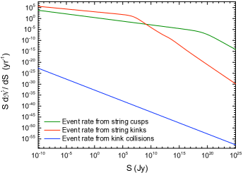
Figure 1: The event rate of radio bursts from superconducting string loops with fixed observed frequency, $\nu_{o}=1.23{\rm GHz}$ as functions of the flux $S$. The green curve corresponds to the case of cusps (the top line in large $S$ regime); the red curve corresponds to the case of kinks (the middle curve in large $S$ regime); and the blue curve corresponds to the case of kink-kink collisions (the bottom curve in large $S$ regime), respectively. We have assumed a single kink on a loop ($N=1$) for these plots. For a different value of $N$, the plots should be rescaled by $N$ for kinks and $N^{2}$ for kink-kink collisions.

We use log-log scale to show the wide range of scales for the flux $S$ in Fig. 1, where it can be seen that the event rate per flux has a power law behavior. For large $S$ values, the event rate from the string cusps is dominant, then is the events from kinks. The contribution of the kink-kink collisions always remains negligible compared to signal from cusps and kinks. As $S$ decreases, the slopes of the curves for cusps and kinks change at certain points, and correspondingly the event rate of kinks catches up and becomes dominant at relatively smaller values of $S$. The blue (the bottom) curve corresponding to kink-kink collisions is the most steep, and thus, one may expect the contribution of kink-kink collisions would be the most important when $S$ is extremely small. However, the parameter space which is detectable by experiments only corresponds to the range of the fluxes where most of the events are due to kinks.

From Fig. 1, we find the asymptotic power law fits for the event rate of radio bursts emitted from cusps, kinks and kink-kink collisions as follows,

$$S\,\frac{d\dot{\mathcal{N}}}{dS}\simeq 2.8\,S_{\rm Jy}^{-1/3}\,\,{\rm yr}^{-1}~{},$$ (cusps) (73)

$$S\,\frac{d\dot{\mathcal{N}}}{dS}\simeq 1.3\times 10^{3}\,N\,S_{\rm Jy}^{-1/4}\,\,{\rm yr}^{-1}~{},$$ (kinks) (74)

$$S\,\frac{d\dot{\mathcal{N}}}{dS}\simeq 2.0\times 10^{-33}\,N^{2}\,S_{\rm Jy}^{-1}\,\,{\rm yr}^{-1}~{},$$ (k-k) (75)

where $S_{\rm Jy}\equiv S/(\rm{1\,Jy})$ and $N$ is the typical number of kinks per loop (conservatively taken to be one in the plot). Hence, an experiment that integrates events over the ranges of $\Delta$ in Eq. (71), and is sensitive to milli Jansky fluxes, will observe about one hundred radio bursts per day from kinks, about one event per day from cusps, and kink-kink collisions cannot produce observable events if there are superconducting cosmic strings with the chosen parameters. If such events are not seen in a search for cosmological radio transients, we will be able to place stringent constraints on superconducting cosmic string parameters. If we consider radio bursts emitted by kinks on superconducting strings with observable frequency $1.23{\rm GHz}$ and flux greater than $300~{}{\rm mJy}$, the event rate is about 0.75 per hour, which is a factor of $30$ larger than the upper bound given by the Parkes survey, $0.025$ per hour. This result implies that current radio experiments might already rule out an interesting part of parameter space given by the current on the string, ${\cal I}$ and the string tension, $G\mu$.

VI.2 Theoretical parameters

In this section, we numerically study the event rates as functions of theoretical parameters, i.e., the current, ${\cal I}$, and the string tension, $G\mu$.

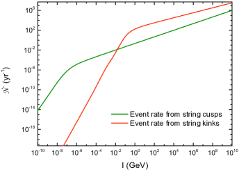
Figure 2: The event rates of radio bursts from cusps and kinks (for one kink/loop) on superconducting string loops at fixed observed frequency, $\nu_{o}=1.23{\rm GHz}$, as functions of the current ${\cal I}$. The string tension is taken to be $G\mu=10^{-10}$. The green curve corresponds to the case of cusps and gives a smaller event rate at high ${\cal I}$; the red curve corresponds to the case of kinks and gives a smaller event rate at lower values of ${\cal I}$. The event rates for kinks should be rescaled by $N$ if there are $N$ kinks per loop.

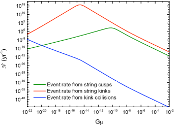
Figure 3: The event rate of radio bursts from superconducting string loops with fixed observed frequency, $\nu_{o}=1.23{\rm GHz}$ as functions of $G\mu$. The current is taken to be $I=10^{5}~{}{\rm GeV}$. The green curve (middle curve at high $G\mu$) corresponds to the case of cusps; the red curve with largest event rate corresponds to the case of kinks; the blue curve corresponds to the case of kink-kink collision and gives a sub-dominant contribution at large $G\mu$. The event rates for kinks and kink-kink collisions should be rescaled by $N$ and $N^{2}$ if there are $N$ kinks per loop.

Fig. 2 shows the total event rate dependence on the current, ${\cal I}$, as a power law. From Fig. 2, we find the asymptotic power law fits at large current values for the event rate of radio bursts from cusps and kinks as follows,

$$\dot{\mathcal{N}}\simeq 4.8\times 10^{2}\,{\cal I}_{5}^{2/3}\,{\rm yr}^{-1}\ ,$$ (cusps) (76)

$$\dot{\mathcal{N}}\simeq 1.1\times 10^{5}\,N\,{\cal I}_{5}^{1/2}\,{\rm yr}^{-1}\ ,$$ (kinks) (77)

where ${\cal I}_{5}\equiv{\cal I}/({\rm 10^{5}\,GeV})$. In the figure, we did not show the dependence of the current in the case of kink-kink collisions since this case do not produce observable signal.

Note that the plots in Figs. 1-3, are obtained by integrating over the duration, which is theoretically constrained to be in the interval $\Delta\in(\Delta_{\min},\Delta_{\max})$ [see the discussion below Eq. (53)], and also experimentally constrained due to the sensitivity of a particular radio transient search. For example, for the Parkes survey, $\Delta_{\min}=10^{-3}$. In the numerical evaluation of the event rate we have used the intersection of the theoretical and experimental ranges of the duration.

Fig. 3 shows the total event rate dependence on $G\mu$. The event rate in the case of cusps and kinks has a maximum at particular values of $G\mu$, namely, $G\mu\sim 10^{-10}$ for cusps and $G\mu\sim 10^{-15}$ for kinks. The maximum occurs because at small string tension electromagnetic radiation is the dominant energy loss mechanism, while at large tension gravitational losses dominate. Further, the event rate from cusps and kinks depend differently on the duration and flux — see Eq. (62) — which causes their curves in the integrated event rate in Fig. 3 to bend over at different values of the tension, depending on the regimes $L(S,\Delta)\gg\Gamma G\mu t$ or $L(S,\Delta)\ll\Gamma G\mu t$.

VII Conclusions

Current carrying superconducting cosmic strings will give three kinds of transient electromagnetic bursts. Bursts from cusps are strong and highly beamed, while bursts from kinks are weaker and less beamed, and the bursts from kink-kink collisions are weakest and not beamed. Only the bursts from cusps and kinks are strong enough to be observed.

The bursts from cusps and kinks occur in all frequency bands but the width of the beams falls off with frequency. Thus the beams are wide in radio, and thin in gamma rays. So the event rate for bursts is largest in the radio bands, which is why the search for radio transients is the most likely to find bursts from superconducting strings.

The search for radio bursts involves several parameters. First is the frequency at which observations are carried out, second is the lower cutoff in flux that the experiment is sensitive to, and the third is the duration of the burst. If we assume some canonical values for the radio frequency and range of burst durations, we can predict the event rate of radio transients from superconducting strings as seen in Fig. 1. The event rate is quite high, at the level of several a day at 1 Jy flux for the choice of string parameters, and should be within easy reach of current efforts. If no bursts are seen, their absence can be used to constrain the string parameters $G\mu$ and ${\cal I}$.

Bursts from superconducting strings can be distinguished from bursts from astrophysical sources as they are linearly polarized, and should have characteristic frequency dependence. In principle, the radio burst is accompanied by bursts at other frequencies but, since the beams at higher frequencies are narrower, they can miss detection. A radio burst should also be accompanied by gravitational wave bursts, but this can be very hard to detect if the string is light. In some string models, there should also be an accompanying burst of neutrinos.

In our analysis, we have made some assumptions that we now spell out. The first is that all strings carry the same uniform current. This assumes that the cosmological medium is magnetized and that the current on strings has built up to its microscopically determined saturation value. If there is a distribution of currents, there will be an additional variable in the distribution of bursts that can affect the event rate. A second assumption is that the radiation backreaction does not drastically change the network properties. We have already accounted for some effects of backreaction. For example, loops evaporate with a certain lifetime due to radiation. However, it is also possible that backreaction prevents cusps from reappearing in every loop oscillation, or that kinks smooth out very rapidly. We have not considered these effects.

- (1) T. W. B. Kibble, “Topology of Cosmic Domains and Strings”, J. Phys. A A 9, 1387 (1976).
- (2) A. Vilenkin and E.P.S. Shellard, “Cosmic Strings and Other Topological Defects”, Cambrigde University Press (1994).
- (3) T. Vachaspati, “Kinks and domain walls: An introduction to classical and quantum solitons,” Cambridge University Press (2006).
- (4) J. Polchinski, “Introduction to cosmic F- and D-strings”, [arXiv: hep-th/0412244].
- (5) E.J. Copeland and T.W.B. Kibble, “Cosmic Strings and Superstrings”, Proc. Roy. Soc. Lond. A 466, 623 (2010) [arXiv : hep-th/0911.1345].
- (6) C. Ringeval, Adv. Astron. 2010 (2010) 380507 [arXiv:1005.4842 [astro-ph.CO]].
- (7) E.J. Copeland, L. Pogosian and T. Vachaspati, “Seeing String Theory in the Cosmos”, Class. Quant. Grav. 28, 204009 (2011) [arXiv:1105.0207].
- (8) E. Witten,“Superconducting Strings”, Nucl. Phys. B 249, 557 (1985).
- (9) A. Vilenkin and T. Vachaspati, “Electromagnetic Radiation from Superconducting Cosmic Strings”, Phys. Rev. Lett. 58, 1041 (1987).
- (10) D. Garfinkle and T. Vachaspati, “Radiation From Kinky, Cuspless Cosmic Loops”, Phys. Rev. D 36, 2229 (1987).
- (11) D. Garfinkle and T. Vachaspati, “Fields Due To Kinky, Cuspless, Cosmic Loops”, Phys. Rev. D 37 (1988) 257.
- (12) T. Vachaspati, “Cosmic Sparks from Superconducting Strings”, Phys. Rev. Lett. 101, 141301 (2008) [arXiv: 0802.0711].
- (13) Y.F. Cai, E. Sabancilar, T. Vachaspati, “Radio bursts from superconducting strings”, Phys. Rev. D 85 023530 (2012) [arXiv: 1110.1631].
- (14) A. Babul, B. Paczynski and D.N. Spergel, Ap. J. Lett. 316, L49 (1987).
- (15) V. Berezinsky, B. Hnatyk and A. Vilenkin, “Gamma-ray bursts from superconducting cosmic strings”, Phys. Rev. D 64 043004 (2001) [arXiv: astro-ph/0102366].
- (16) K. S. Cheng, Y. -W. Yu and T. Harko, “High Redshift Gamma-Ray Bursts: Observational Signatures of Superconducting Cosmic Strings?”, Phys. Rev. Lett. 104, 241102 (2010) [arXiv:1005.3427].
- (17) D. R. Lorimer, M. Bailes, M. A. McLaughlin, D. J. Narkevic and F. Crawford, “A bright millisecond radio burst of extragalactic origin”, Science 318, 777 (2007) [arXiv:0709.4301 [astro-ph]].
- (18) C. D. Patterson et al., “Searching for Transient Pulses with the ETA Radio Telescope”, ACM Trans. Reconf. Tech. Syst. 1, 1 (2009) [arXiv:0812.1255 [astro-ph]].
- (19) P. Henning et al., “The First Station of the Long Wavelength Array”, PoS ISKAF 2010, 024 (2010) [arXiv:1009.0666 [astro-ph.IM]].
- (20) R. Fender et al., (The LOFAR Collaboration), “The LOFAR Transients Key Project”, PoS MQW6, 104 (2006) [arXiv:astro-ph/0611298]; “LOFAR Transients and the Radio Sky Monitor”, PoS DYNAMIC, 030 (2007) [arXiv:0805.4349 [astro-ph]].
- (21) J. M. Cordes, “Radio Transients and the SKA as a Synoptic Survey Facility”, Bull. Amer. Astron. Soc. Vol. 39, 999 (2007); P. E. Dewdney et al., “The Square Kilometer Array”, Proc. IEEE Vol. 97, 1482 (2009).
- (22) V. Berezinsky, K.D. Olum, E. Sabancilar and A. Vilenkin, “UHE neutrinos from superconducting cosmic strings”, Phys. Rev. D 80, 023014 (2009) [arXiv:0901.0527].
- (23) T. Damour and A. Vilenkin, “Gravitational wave bursts from cosmic strings”, Phys. Rev. Lett. 85, 3761 (2000) [arXiv:gr-qc/0004075]; “Gravitational wave bursts from cusps and kinks on cosmic strings”, Phys. Rev. D 64, 064008 (2001) [arXiv:gr-qc/0104026]; “Gravitational radiation from cosmic (super)strings: Bursts, stochastic background, and observational windows”, Phys. Rev. D 71, 063510 (2005) [arXiv:hep-th/0410222].
- (24) J. Abadie et al., [The LIGO Scientific Collaboration and the Virgo Collaboration], “Implementation and testing of the first prompt search for electromagnetic counterparts to gravitational wave transients” [arXiv: 1109.3498].
- (25) E. Komatsu et al. [WMAP Collaboration], “Seven-Year Wilkinson Microwave Anisotropy Probe (WMAP) Observations: Cosmological Interpretation”, Astrophys. J. Suppl. 192, 18 (2011) [arXiv:1001.4538 [astro-ph.CO]].
- (26) R. Keisler, C. L. Reichardt, K. A. Aird, B. A. Benson, L. E. Bleem, J. E. Carlstrom, C. L. Chang and H. M. Cho et al., “A Measurement of the Damping Tail of the Cosmic Microwave Background Power Spectrum with the South Pole Telescope”, Astrophys. J. 743, 28 (2011) [arXiv:1105.3182 [astro-ph.CO]].
- (27) C. Dvorkin, M. Wyman and W. Hu, “Cosmic String constraints from WMAP and the South Pole Telescope”, Phys. Rev. D 84, 123519 (2011) [arXiv:1109.4947].
- (28) T. Vachaspati and A. Vilenkin, “Gravitational Radiation From Cosmic Strings”, Phys. Rev. D 31, 3052 (1985).
- (29) R. van Haasteren et al., “Placing limits on the stochastic gravitational wave backgroung using European pulsar timing array data” [arXiv: astro-ph.CO/1103.0576].
- (30) S. Olmez, V. Mandic and X. Siemens, “Gravitational-wave stochastic background from kinks and cusps on cosmic strings”, Phys. Rev. D81, 104028 (2010).
- (31) S.A. Sanidas, R.A. Battye and B.W. Stappers, “Constraints on cosmic string tension imposed by the limit on the stochastic gravitational wave background from the European Pulsar Timing Array” [arXiv:1201.2419].
- (32) P. Binetruy, A. Bohe, C. Caprini and J.-F. Dufaux, “Cosmological Backgrounds of Gravitational Waves and eLISA/NGO: Phase Transitions, Cosmic Strings and Other Sources.” [arXiv:1201.0983].
- (33) I. Sendra and T. L. Smith, “Improved limits on short-wavelength gravitational waves from the cosmic microwave background”, [arXiv: 1203.4232].
- (34) R. Sunyaev and Y. Zeldovich, Ann. Rev. Astron. Astrophys. 18, 537 (1980).
- (35) J. C. Mather et al., Astrophys. J. 420, 439 (1994); D. Fixsen, E. Cheng, J. Gales, J. C. Mather, R. Shafer, et al., Astrophys. J. 473, 576 (1996).
- (36) N.G. Sanchez, M. Signore, Phys. Lett. B219, 413 (1989).
- (37) N.G. Sanchez, M. Signore, Phys. Lett. B241 332 (1990).
- (38) H. Tashiro, E. Sabancilar and T. Vachaspati, “CMB Distortions from Superconducting Cosmic Strings” [arXiv:1202.2474].
- (39) A. Kogut, D. Fixsen, D. Chuss, J. Dotson, E. Dwek, et al., JCAP 1107, 025 (2011).
- (40) H. Tashiro, E. Sabancilar and T. Vachaspati, “Constraints on Superconducting Cosmic Strings from Early Reionization”, [arXiv: 1204.3643].
- (41) D. A. Steer and T. Vachaspati, Phys. Rev. D 83, 043528 (2011) [arXiv:1012.1998 [hep-th]].
- (42) J. J. Blanco-Pillado and K. D. Olum, Nucl. Phys. B 599, 435 (2001) [arXiv:astro-ph/0008297 [astro-ph]].
- (43) S. Weinberg, “Gravitation and Cosmology: Principles and Applications of the General Theory of Relativity”, John Wiley and Sons (1972).
- (44) D.P. Bennett and F.R. Bouchet, Phys. Rev. D 41, 2408 (1990).
- (45) B. Allen and E.P.S. Shellard, Phys. Rev. Lett. 64, 119 (1990).
- (46) G.R. Vincent, M. Hindmarsh and M. Sakellariadou, Phys. Rev. D 56, 637 (1997).
- (47) C.J.A.P. Martins and E.P.S. Shellard, Phys. Rev. D 73, 043515 (2006).
- (48) C. Ringeval, M. Sakellariadou and F. Bouchet, JCAP 0702, 023 (2007).
- (49) V. Vanchurin, K.D. Olum and A. Vilenkin, Phys. Rev. D 74, 063527 (2006).
- (50) K.D. Olum and V. Vanchurin, Phys. Rev. D 75, 063521 (2007).
- (51) J.J. Blanco-Pillado,K.D. Olum and B. Shlaer, Journal of Computational Physics 231 98 (2012).
- (52) J.J. Blanco-Pillado, K.D. Olum and B. Shlaer, Phys. Rev. D 83, 083514 (2011) [arXiv : astro-ph.CO/1101.5173].
- (53) J.V. Rocha, “Scaling solution for small cosmic string loops”, Phys. Rev. Lett. 100, 071601 (2008) [arXiv: 0709.3284].
- (54) J. Polchinski and J.V. Rocha, Phys. Rev. D 75, 123503 (2007).
- (55) F. Dubath, J. Polchinski and J.V. Rocha, Phys. Rev. D 77, 123528 (2008).
- (56) V. Vanchurin, “Towards a kinetic theory of strings”, Phys. Rev. D 83, 103525 (2011) [arXiv: 1103.1593].
- (57) L. Lorenz, C. Ringeval and M. Sakellariadou, “Cosmic string loop distribution on all length scales and at any redshift”, JCAP 1010, 003 (2010) [arXiv:1006.0931].
- (58) C. J. Copi and T. Vachaspati, Phys. Rev. D 83, 023529 (2011) [arXiv:1010.4030 [hep-th]].
- (59) G. B. Rybicki and A. P. Lightman, Radiative Processes in Astrophysics (Wiley, New York, 1979).
- (60) L. C. Lee and J. R. Jokipii, Ap. J. 206, 735 (1976).
- (61) S. R. Kulkarni, E. O. Ofek, J. D. Neill, M. Juric and Z. Zheng, “Giant Sparks at Cosmological Distances,” unpublished (2007).
- (62) B. J. Rickett, Ann. Rev. Astron. Astrophys. 15, 479-504 (1977).