Universal reference state in a driven homogeneous granular gas

Abstract

We study the dynamics of a homogeneous granular gas heated by a stochastic thermostat, in the low density limit. It is found that, before reaching the stationary regime, the system quickly “forgets” the initial condition and then evolves through a universal state that does not only depend on the dimensionless velocity, but also on the instantaneous temperature, suitably renormalized by its steady state value. We find excellent agreement between the theoretical predictions at Boltzmann equation level for the one-particle distribution function, and Direct Monte Carlo simulations. We conclude that at variance with the homogeneous cooling phenomenology, the velocity statistics should not be envisioned as a single-parameter, but as a two-parameter scaling form, keeping track of the distance to stationarity.

I Introduction

A granular gas may be viewed as a collection of macroscopic particles undergoing dissipative collisions. This very ingredient –inelasticity– gives rise to a rich phenomenology d00 ; g03 ; BP04 ; at06 , the understanding of which requires statistical mechanics tools: Kinetic theory has proven to be powerful at a microscopic/mesoscopic level of description, while at a macroscopic scale, hydrodynamic equations have been derived g03 and put to the test. Yet, the relevance and consistency of a hydrodynamic framework, which is a central question, is still elusive k99 ; g01 ; d01 .

Due to collisional dissipation, the granular temperature, defined as the variance of velocity fluctuations, decays monotonically in time in an isolated granular system h83 . In the fast-flow regime, it has been shown numerically that for a wide class of initial conditions, the system reaches a homogeneous state in which all the time dependence of the one-particle distribution function is encoded in the temperature. This is the so-called homogeneous cooling state (HCS) which has been widely studied in the literature gs95 ; vne98 . In such a homogeneous situation, the dynamics involves two time-scales: the kinetic or fast scale –a few collisions per particle– in which the scaling regime has not been reached yet and where the “microscopic” excitations relax, and the following hydrodynamic or slow scale in which the memory of initial conditions has been lost, and the velocity distribution evolves through the granular temperature bdr03 . Considering non homogeneous states, this separation of time scales opens the possibility of a hydrodynamic or coarse-grained description in terms of the density, velocity and temperature field, and the HCS then plays the role of the reference state when the Chapmann-Enskog method is applied bdks98 .

On the other hand, several studies and experiments in granular matter deal with stationary states, which are reached under the action of some energy driving, often realized by a moving boundary, or by an interstitial medium that acts as a thermostat, see e.g. PEU02 ; L09 ; PGG12 . In all these cases, the energy injected compensates for the energy lost in collisions. From a theoretical point of view, a minimalistic approach is to consider the system as driven by some random energy source, which can be implemented in different ways clh00 . For the hard particle model, one of the most used homogeneous heating is the so-called stochastic thermostat, which consists in a white noise force acting on each grain wm96 ; vne98 ; vnetp99 ; MS00 ; P02 ; gm02 ; V06 ; V06bis ; M09 ; M09bis ; VL11 ; plmv99 . In the low density limit, the distribution function of the homogeneous state has been characterized vne98 . Hydrodynamic equations have been derived via the Chapmann-Enskog expansion gm02 and fluctuating hydrodynamics have been put forward in order to understand the large scale structure found in the stationary state vnetp99 , or fluctuations of global quantities M09bis . We stress that in all the studies pertaining to the hydrodynamics of a system heated by the stochastic thermostat vnetp99 ; gm02 , the stationary state played the role of “reference” state, as the HCS happens to be in the undriven case. It was therefore assumed that a one parameter scaling holds for the velocity probability distribution. The objective in this work is to analyze this point critically in the homogeneous case at the level of the Boltzmann equation. We will study, for arbitrary initial conditions, the type of state the system evolves into in a kinetic time scale. Surprisingly, we find that a universal state is reached in a kinetic scale –universal in the sense that it is independent of the initial conditions– but that depends on the quotient between the instantaneous temperature and its stationary value.

The outline is as follows. Section II opens with a definition of the model, and a summary of relevant previously known results. The key question addressed lies in the scaling form of the velocity distribution close to the steady state. Does it depend only on the suitably reduced velocity variable, as is the case in the HCS, or is another parameter relevant, that would encode the distance to stationarity ? We will argue in section II.1 that a single parameter scaling form is inconsistent. We shall then show in sections II.2 and II.3 that a consistent two parameter scaling form can be identified. Its properties will be characterized by complementary numerical and analytical tools. Conclusions and perspectives will finally be discussed in section III.

II Scaling form of the velocity distribution function

The system of interest is a dilute gas of $N$ smooth inelastic hard particles of mass $m$ and diameter $\sigma$, which collide inelastically with a coefficient of normal restitution $\alpha$ independent of the relative velocity BP04 . If at time $t$ there is a binary encounter between particles $i$ and $j$, having velocities $\mathbf{V}_{i}(t)$ and $\mathbf{V}_{j}(t)$ respectively, the post-collisional velocities $\mathbf{V}_{i}^{\prime}(t)$ and $\mathbf{V}_{j}^{\prime}(t)$ are

$$\mathbf{V}_{i}^{\prime} = \mathbf{V}_{i}-\frac{1+\alpha}{2}(\hat{\boldsymbol{\sigma}}\cdot\mathbf{V}_{ij})\hat{\boldsymbol{\sigma}},$$

$$\mathbf{V}_{j}^{\prime} = \mathbf{V}_{j}+\frac{1+\alpha}{2}(\hat{\boldsymbol{\sigma}}\cdot\mathbf{V}_{ij})\hat{\boldsymbol{\sigma}},$$ (1)

where $\mathbf{V}_{ij}\equiv\mathbf{V}_{i}-\mathbf{V}_{j}$ is the relative velocity and $\hat{\boldsymbol{\sigma}}$ is the unit vector pointing from the center of particle $j$ to the center of particle $i$ at contact. Between collisions, the system is heated uniformly by a white noise acting independently on each grain vne98 ; vnetp99 ; P02 ; gm02 ; V06 ; M09 ; M09bis so that the one-particle velocity distribution, $f(\mathbf{r},\mathbf{v},t)$, then obeys the Boltzmann-Fokker-Planck equation vne98 ; vk92 . For a homogeneous system this equation reads

$$\frac{\partial}{\partial t}f(\mathbf{v}_{1},t)=\sigma^{d-1}\int d\mathbf{v}_{2}\bar{T}_{0}(\mathbf{v}_{1},\mathbf{v}_{2})f(\mathbf{v}_{1},t)f(\mathbf{v}_{2},t)+\frac{\xi_{0}^{2}}{2}\frac{\partial^{2}}{\partial\mathbf{v}_{1}^{2}}f(\mathbf{v}_{1},t),$$ (2)

where $d$ is the dimension of space, $\xi_{0}$ measures the noise strength, and $\bar{T}_{0}$ is the binary collision operator

$$\bar{T}_{0}(\mathbf{v}_{1},\mathbf{v}_{2})=\int d\hat{\boldsymbol{\sigma}}\Theta(\mathbf{v}_{12}\cdot\hat{\boldsymbol{\sigma}})(\mathbf{v}_{12}\cdot\hat{\boldsymbol{\sigma}})(\alpha^{-2}b_{\sigma}^{-1}-1).$$ (3)

Here we have introduced the operator $b_{\sigma}^{-1}$ which replaces the velocities $\mathbf{v}_{1}$ and $\mathbf{v}_{2}$ by the precollisional ones $\mathbf{v}_{1}^{*}$ and $\mathbf{v}_{2}^{*}$ given by

$$\mathbf{v}_{1}^{*} = \mathbf{v}_{1}-\frac{1+\alpha}{2\alpha}(\hat{\boldsymbol{\sigma}}\cdot\mathbf{v}_{12})\hat{\boldsymbol{\sigma}},$$

$$\mathbf{v}_{2}^{*} = \mathbf{v}_{2}+\frac{1+\alpha}{2\alpha}(\hat{\boldsymbol{\sigma}}\cdot\mathbf{v}_{12})\hat{\boldsymbol{\sigma}}.$$ (4)

II.1 One-parameter scaling or beyond ?

It is an observation from numerical simulations, that for a wide class of initial conditions the system reaches a stationary state vne98 ; vnetp99 ; P02 . Assuming that total momentum is zero, i.e. $\int d\mathbf{v}\mathbf{v}f(\mathbf{v},0)=\mathbf{0}$, the state is characterized by an isotropic stationary distribution, $f_{s}(v)$. Let us define the scaled distribution function, $\chi_{s}$, by

$$f_{s}(v)=\frac{n}{v_{s}^{d}}\chi_{s}(c),\qquad\mathbf{c}=\frac{\mathbf{v}}{v_{s}},$$ (5)

where $n$ is the density, $v_{s}\equiv\sqrt{2T_{s}/m}$ is the thermal velocity and $T_{s}$ is the stationary temperature, $\frac{d}{2}nT_{s}=\int d\mathbf{v}\frac{1}{2}mv^{2}f_{s}(\mathbf{v})$. As $\chi_{s}$ is rather close to a Maxwellian distribution, a reasonable strategy is to perform an expansion in Sonine polynomials resibois . In the so-called first Sonine approximation, the steady state function then reads vne98

$$\chi_{s}(c)\approx\chi_{M}(c)[1+a_{2}^{s}S_{2}(c^{2})],$$ (6)

where $\chi_{M}$ is the Maxwellian distribution with unit temperature, $S_{2}(c^{2})=\frac{d(d+2)}{8}-\frac{d+2}{2}c^{2}+\frac{1}{2}c^{4}$, is the second Sonine polynomial, and $a_{2}^{s}$ is the kurtosis of the distribution. Within this approximation, the distribution function can be calculated, with the result vne98

$$a_{2}^{s}(\alpha)=\frac{16(1-\alpha)(1-2\alpha^{2})}{73+56d-24d\alpha-105\alpha+30(1-\alpha)\alpha^{2}},$$ (7)

and a stationary temperature

$$T_{s}=m\left[\frac{d\Gamma(d/2)\xi_{o}^{2}}{2\pi^{\frac{d-1}{2}}(1-\alpha^{2})n\sigma^{d-1}}\right]^{2/3}.$$ (8)

Now, let us consider an initial condition with a temperature that differs appreciably from the stationary temperature (we also assume that total momentum is zero, its precise value being immaterial). It is clear that the system will reach the stationary state in a hydrodynamic scale. The ensuing question is two-pronged. First of all, is the dynamics compatible with a universal scaling form –once the memory of initial condition is lost– that would provide a consistent solution to the Boltzmann equation, or is memory only washed out strictly speaking at the steady state point? Second, assuming such a scaling regime exists in some vicinity of the steady state, what is the minimal number of parameters required for its description? By analogy with unforced (HCS) phenomenology, a single parameter scaling might be anticipated:

$$f(\mathbf{v},t)=\frac{n}{v_{o}^{d}(t)}\chi_{s}(c)\quad\hbox{where}\quad\mathbf{c}\equiv\mathbf{v}/v_{0}(t)\quad\hbox{and}\quad v_{0}(t)\equiv\sqrt{2T(t)/m}$$ (9)

is defined from the instantaneous temperature $dnT(t)=\int d\mathbf{v}mv^{2}f(\mathbf{v},t)$. We note that this scaling property holds for the Gaussian thermostat as well MS00 , where the particles are accelerated between collisions by a force proportional to its own velocity gT . Moreover, in the stochastic thermostat case, the one parameter scaling (9) was implicitly assumed, and it seemed to be yield reasonable predictions at least close to the stationary state, see vnetp99 ; gm02 . Nevertheless, when the form (9) is inserted in the Boltzmann equation, Eq. (2), we obtain

$$\frac{\xi_{0}^{2}}{2v_{0}^{3}(t)}\frac{\partial^{2}}{\partial\mathbf{c}_{1}^{2}}\chi_{s}(c_{1})+\frac{1}{v_{0}^{2}(t)}\frac{dv_{0}(t)}{dt}\frac{\partial}{\partial\mathbf{c}_{1}}\cdot[\mathbf{c}_{1}\chi_{s}(c_{1})]=-n\sigma^{d-1}\int d\mathbf{c}_{2}\bar{T}_{0}(\mathbf{c}_{1},\mathbf{c}_{2})\chi_{s}(c_{1})\chi_{s}(c_{2}),$$ (10)

which is inconsistent: The left hand side depends on time while the right hand side does not. We conclude that such a solution should be ruled out, except when stationarity is reached and $v_{0}=v_{s}$. The hope is to capture the post-kinetic time dependence of $f(\mathbf{v},t)$, through a more involved functional form, that would be free of the above inconsistency.

As is customary, we shall seek for a normal solution resibois , which in the present homogeneous case means that $f(\mathbf{v},t)$ should only depend on time via the instantaneous granular temperature $T(t)$. In conjunction with dimensional analysis, this leads to a function that should only depend on $\mathbf{c}$ and $T(t)/T_{s}=v_{0}^{2}/v_{s}^{2}$, which we write as

$$f(\mathbf{v},t)=\frac{n}{v_{0}^{d}(t)}\chi(c,\beta),\quad\hbox{with}\quad\beta\equiv\frac{v_{s}}{v_{0}(t)}$$ (11)

and again $\mathbf{c}=\mathbf{v}/v_{0}(t)$. Note that we have assumed isotropy, $\chi$ depending on $c=|\mathbf{c}|$ and not on the full vector $\mathbf{c}$, but this assumption can be easily relaxed. Note also that equivalent expressions can of course be chosen, such as $\tilde{\chi}(v/v_{s},\beta)$.

If a state such as (11) holds, it represent a strong constraint on the form of the velocity distribution. The corresponding dynamics can be partitioned in a first rapid stage –that we do not attempt to describe– where initial conditions matter, and a subsequent universal relaxation towards stationarity, where only the distance to the steady state is relevant, through the dimensionless inverse typical velocity $\beta=v_{s}/v_{0}(t)$.

II.2 Numerical simulations answer

To put the above scenario to the test, we have performed Direct Monte Carlo Simulations (DSMC) bird of $N=1000$ hard disks ($d=2$) of unit mass and unit diameter, that collide inelastically with the collision rule given by equation (II). The thermostat is implemented following previous investigations vnetp99 and the results have been averaged over $10^{5}$ trajectories. For a given value of the inelasticity, we thus solve the time-dependent Boltzmann equation for different initial conditions and analyze whether, after some kinetic transient, all the time dependence of the distribution function goes through the dimensionless parameter $\beta$. As it is difficult to measure the complete distribution function with the desired accuracy, we have worked with the cumulants of the scaled distribution, $\chi(\mathbf{c},\beta)$. In terms of the velocity moments, $\langle v^{l}\rangle\equiv\frac{1}{n}\int d\mathbf{v}v^{l}f(\mathbf{v},t)$, we have measured the kurtosis of the distribution

$$a_{2}=\frac{d}{d+2}\frac{\langle v^{4}\rangle}{\langle v^{2}\rangle^{2}}-1,$$ (12)

which is proportional to the fourth cumulant of $\chi(\mathbf{c},\beta)$ and the quantity

$$a_{3}=-\frac{d^{2}}{(d+2)(d+4)}\frac{\langle v^{6}\rangle}{\langle v^{2}\rangle^{3}}+\frac{3d}{d+2}\frac{\langle v^{4}\rangle}{\langle v^{2}\rangle^{2}}-2,$$ (13)

which can be viewed as the reduced sixth cumulant. If our scaling is correct, we expect that the cumulants quickly collapse for different initial conditions, as a function of $\beta$. In Fig. 1, we have plotted $a_{2}$ and $a_{3}$ versus $\beta$ for $\alpha=0.95$. The initial conditions are either Maxwellian distributions with three different temperatures $T_{0}$, significantly above the steady state value $T_{s}$, or asymmetric distributions made up of three possible velocities with different probabilities

$$f(v_{x},v_{y},t=0) = \frac{3}{6}\delta\left(v_{x}+8D/3\right)\delta\left(v_{y}+8D/3\right)+\frac{2}{6}\delta\left(v_{x}-4D/3\right)\delta\left(v_{y}-4D/3\right)$$ (14)

$$+ \frac{1}{6}\delta\left(v_{x}-16D/3\right)\delta\left(v_{y}-16D/3\right).$$

Here, the parameter $D$ is chosen to match the initial desired temperature (chosen the same as in the Gaussian initial condition). All the quantities are measured every $250$ collisions, so that each four consecutive points in figure 1 correspond to a time span of one collision per particle. It can be seen that, after some transient, memory of the initial condition is forgotten, so that the stationary distribution ($\beta=1$) is reached following a universal route. In figure 1, those data points associated to the Gaussian initial distribution approach the scaling curve from above (circles) while those for the initial asymmetric case (14) approach the scaling curve from below (squares). A very similar behavior can be seen in Fig 2 for $\alpha=0.8$ and four different initial temperatures, again such that $T_{0}\gg T_{s}$, which ensures that $\beta<1$ (we have also probed the regime $\beta>1$ obtained with $T_{0}\ll T_{s}$, where similar conclusions hold, see e.g. Fig. 4 below). We have started either with a Maxwellian distribution, as above, or with a distribution in which all the velocities have the same probability density in a square centered on $\mathbf{v}=\mathbf{0}$ (referred to as the “flat” case). We emphasize that the initial transient is fast: memory of the initial condition is lost after at most $3$ or $4$ collisions per particle, a phenomenon that cannot be appreciated from the figures.

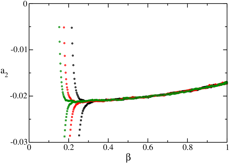
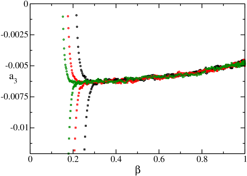
Figure 1: Coefficients $a_{2}$ and $a_{3}$ from Monte Carlo, for $\alpha=0.95$. We start with a Maxwellian (circles) or asymmetric (squares) distribution, and three initial temperatures: $T_{0}/T_{s}=22,33,44$. Note the vertical scale.

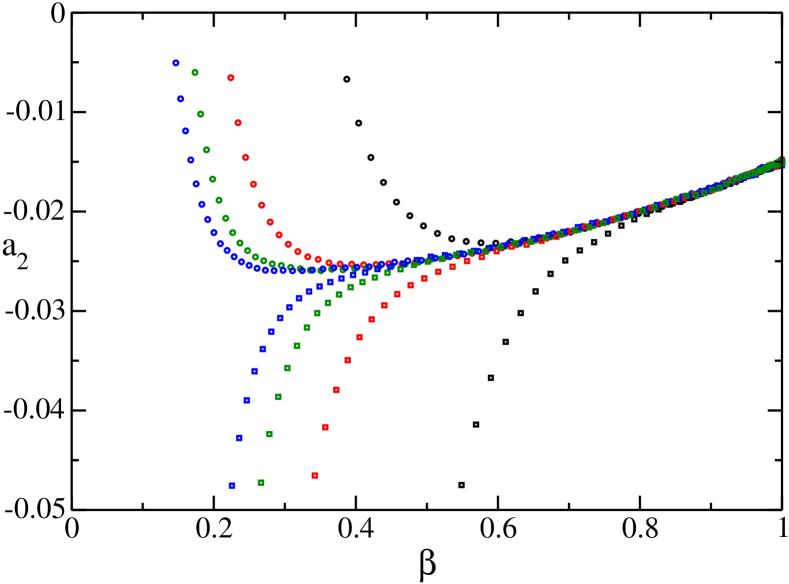
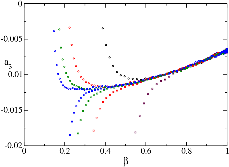
Figure 2: Same as Fig 1, but for a more dissipative system with restitution coefficient $\alpha=0.8$. Here, the initial condition is either Gaussian (circles, approaching the master curve from above), or flat (squares, see text, approaching the master curve from below). In both cases, the initial temperature is $T_{0}/T_{s}=7.3,21.8,36.4$ and 51.

Borrowing ideas from the extended self-similarity technique B93 , we put to the test the possibility of an enhanced universality, by plotting $a_{3}$ as a function of $a_{2}$, see Fig. 3. In doing so, it appears that the universal part of the $a_{i}$ versus $\beta$ curve seen in Fig. 1 is not enhanced by the reparametrization $a_{3}(a_{2})$: different initial conditions do not lead to a data collapse, beyond the interval $-0.22<a_{2}<-0.17$ that was already evidenced in Fig. 1. However, a given functional form (say Maxwellian) leads to a unique path in the $a_{3}$-$a_{2}$ plane, which is already a non trivial point, and furthermore, a plot like Fig. 3 leads to a significantly reduced scatter of points that Fig. 1. It is therefore more amenable to chart out the universal regime sought for. In these figures, the first measure reported after the dynamics has acted on the initial conditions is for a time of $0.25$ collisions per particle for the Maxwellian distribution and of around $3$ collisions per particle for the flat and asymmetric distributions. The present results establish numerically the existence of a universal non-trivial scaling regime, for which we now seek analytical characterization.

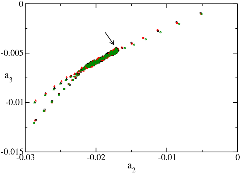
Figure 3: Same data as in Fig. 1, where the coefficient $a_{3}$ is shown as a function of $a_{2}$. In addition to Maxwellian and asymmetric, flat initial conditions are also shown. The arrow indicates the steady state values.

II.3 Analytical approach

For the sake of analytical progress, it is convenient to change variables in the Boltzmann equation (2), from the set $\{t,\mathbf{v}\}$, to $\{\beta,\mathbf{c}\}$. In these variables, the scaled distribution function fulfills

$$[\mu(\beta)-\mu(1)\beta^{3}]\left\{\frac{\partial}{\partial\mathbf{c}_{1}}\cdot[\mathbf{c}_{1}\chi(\mathbf{c}_{1},\beta)]+\beta\frac{\partial}{\partial\beta}\chi(\mathbf{c}_{1},\beta)\right\}$$

$$=\int d\mathbf{c}_{2}\bar{T}_{0}(\mathbf{c}_{1},\mathbf{c}_{2})\chi(\mathbf{c}_{1},\beta)\chi(\mathbf{c}_{2},\beta)+\frac{1}{2}\mu(1)\beta^{3}\frac{\partial^{2}}{\partial\mathbf{c}_{1}^{2}}\chi(\mathbf{c}_{1},\beta),$$ (15)

where

$$\mu(\beta)=-\frac{1}{2d}\int d\mathbf{c}_{1}\int d\mathbf{c}_{2}(c_{1}^{2}+c_{2}^{2})\bar{T}_{0}(\mathbf{c}_{1},\mathbf{c}_{2})\chi(\mathbf{c}_{1},\beta)\chi(\mathbf{c}_{2},\beta).$$ (16)

We note that here and in contrast with Eq. (10), the equation is fully consistent as it appears as a change of variables where $\beta$ simply plays the role of time. Nevertheless, proving that for any “reasonable” initial condition, the system forgets the initial condition and reaches a universal state is a formidable task. For this reason we limit ourselves to the simplified problem of deriving an approximate expression for this distribution function. As in the stationary state, the distribution will be worked out in the first Sonine approximation

$$\chi(c,\beta)\approx\chi_{M}(c)[1+a_{2}(\beta)S_{2}(c^{2})],$$ (17)

where the kurtosis, $a_{2}$, has been defined in (12) and, by definition, we have

$$\int d\mathbf{c}\chi(c,\beta)=1,\qquad\int d\mathbf{c}\mathbf{c}\chi(c,\beta)=\mathbf{0},\qquad\int d\mathbf{c}c^{2}\chi(c,\beta)=\frac{d}{2}.$$ (18)

In expansion (17), we neglect contributions in $a_{3}$ and higher order. This is justified as long as the inelasticity is not too strong, and is backed up here by the fact that $|a_{3}|<a_{2}$, as can be seen in Figs. 1 and 2. Of course, inclusion of higher order terms in (17) would improve the accuracy of the subsequent calculation.

Inserting (17) into the Boltzmann equation (II.3), taking the fourth velocity moment while neglecting nonlinear terms in $a_{2}$, we obtain the following evolution equation for the cumulant $a_{2}$

$$\frac{1}{4}\beta(1-\beta^{3})\frac{d}{d\beta}a_{2}(\beta)=(1-B-\beta^{3})a_{2}(\beta)+Ba_{2}^{s},$$ (19)

where the parameter $B$ depends on dissipation and space dimension according to

$$B=\frac{73+8d(7-3\alpha)+15\alpha[2\alpha(1-\alpha)-7]}{16(1-\alpha)(3+2d+2\alpha^{2})+a_{2}^{s}[85+d(30\alpha-62)+3\alpha(10\alpha(1-\alpha)-39)]}.$$ (20)

Eq. (19) is an inhomogeneous linear differential equation that can be integrated. It exhibits two singular points at $\beta=0$, $\beta=1$, and we start with the interval $[0,1]$. In this case the general solution of the associated homogeneous equation reads

$$a_{2}^{H}(\beta)=K\frac{(1-\beta^{3})^{\frac{4}{3}B}}{\beta^{4(B-1)}}$$ (21)

and a particular solution can be obtained by variations of parameters. The general solution will then be the sum of these two contributions. The ensuing $a_{2}$ depends on the initial conditions through $K$, and since our purpose here is to extract the universal behaviour of $a_{2}$ as a function of $\beta$, we note that the contribution (21) fades rapidly as $\beta$ approaches unity (as $(1-\beta^{3})^{4B/3}$ where $B$ can be large ; note that it diverges in the elastic limit $\alpha\to 1$). The universal behaviour is consequently encoded is the particular solution, and we finally have

$$a_{2}(\beta)=a_{2}^{s}\left[1+\frac{1-\beta^{3}}{B-1}\,_{2}F_{1}\left(-\frac{1}{3},1;\frac{4B-1}{3};\beta^{3}\right)\right],\qquad 0<\beta<1.$$ (22)

where $\,{}_{2}F_{1}$ is the hyper-geometric function arnoldVasilii . This expression is well behaved in all the interval $[0,1]$. An analogous analysis can be performed for $\beta>1$. Following similar lines, we identify the universal solution to be

$$a_{2}(\beta)=-\frac{4Ba_{2}^{s}}{7\beta^{3}(1-1/\beta^{3})^{\frac{4B}{3}}}\,_{2}F_{1}\left(\frac{7}{3},1+\frac{4B}{3};\frac{10}{3};\frac{1}{\beta^{3}}\right).$$ (23)

Clearly, the same technical procedure can be applied to the higher order cumulants. For the sake of simplicity, we restrict to the function $a_{2}(\beta)$, that we wish to test against simulation results.

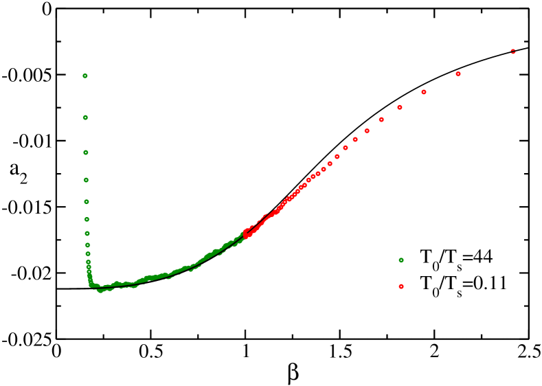
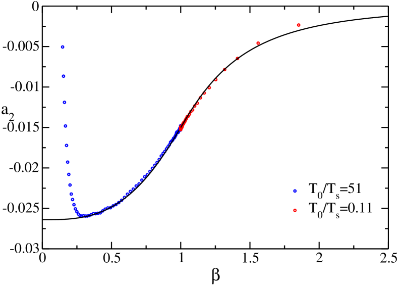
Figure 4: Kurtosis as a function of $\beta$ (reduced inverse typical velocity), for a system with $\alpha=0.95$ (left) and $\alpha=0.80$ (right). The points are simulation results starting from a Maxwellian distribution and the solid line is the theoretical prediction, given by Eq. (22) for $\beta<1$ and Eq. (23) for $\beta>1$, see text. The two values of the initial temperature mentioned for each graph are used to generate separately the $\beta<1$ branch (associated to large $T_{0}$) and the $\beta>1$ branch (obtained for small $T_{0}$). The steady state values correspond to $\beta=1$.

In order to compare the above theoretical predictions to the simulation data, attention should be payed to the fact that analytical computation of velocity moments or cumulants is plagued by non-linear effects that have been discussed in the literature MS00 ; C03 . This results in some error in the calculation of the steady state value $a_{2}^{s}$, and we can also expect $B$ to suffer from a similar inaccuracy, that may be of the order of 10 or 20%. To circumvent this (somewhat minor) drawback, we take $a_{2}^{s}$ appearing in Eqs. (22) and (23) from the Monte Carlo simulations, and we adjust $B$ to match the measured function $a_{2}(\beta)$. This procedure provides us with Fig. 4, where the agreement between the functional forms (22) and (23) with Monte Carlo is excellent. It is of course important to check a posteriori that $a_{2}^{s}$ and $B$ thereby obtained are close enough to our predictions. The precise values are reported below:

$$\begin{array}[]{l || c | c}\hbox{}&\alpha=0.95&\alpha=0.8\\ \hline\cr\hline\cr a_{2}^{s}\hbox{ from DSMC }&-0.0171&-0.0150\\ a_{2}^{s}\hbox{ from Eq. (\ref{eq:a2s}) }&-0.0157&-0.0135\\ \hline\cr B\hbox{ from DSMC }&5.17&2.32\\ B\hbox{ from Eq. (\ref{eq:B}) }&6.43&2.61\end{array}$$ (24)

III Conclusion and perspectives

To summarize, we have studied the dynamics of a system of inelastic hard spherical grains, heated homogeneously by a stochastic thermostat. We have restricted the analysis to low density systems, amenable to a Boltzmann equation treatment. We have found that generically, after a kinetic transient, the system evolves into a scaling solution that no longer depends on initial conditions, before the steady state is finally reached. The relevant scaling form is not of the single parameter family as is the case in the homogeneous cooling state, but involves 2 parameters. The velocity distribution function was calculated in the so-called first Sonine approximation, which provides a very good agreement with the Monte Carlo simulations.

At this point several questions arise: What is the counterpart of the universal state brought to the fore at two-particle level, or even $N$-particle ? What is the effect of density, and of a change in the driving mechanism ? Do the hydrodynamic relations (worked out say at Chapman Enskog level) depend on the structure of this state? The complete answer to all these interrogations requires further studies, but we expect that similar scaling forms should occur at higher densities, and with different thermostats as long as a steady state can be reached. In this respect, the Gaussian thermostat is presumably singular, since it can be mapped onto the free cooling case. The questions pertaining to hydrodynamics are more subtle; How the universal $\beta$-scaling behaviour discussed in the present work impinges, as a reference state, on transport properties, should be explored.

IV Acknowledgments

This research was supported by the Ministerio de Educación y Ciencia (Spain) through Grant No. FIS2008-01339 (partially financed by FEDER funds).

References

- (1) J. W. Dufty, J. Phys.: Condens. Matter 12, A47 (2000).
- (2) I. Goldhirsch, Annu. Rev. Fluid Mech. 35, 267 (2003).
- (3) N. Brilliantov and T. Pöschel, Kinetic Theory of Granular Gases (Clarendon Press, Oxford, 2004).
- (4) I. S. Aranson and L. S. Tsimring, Rev. Mod. Phys. 78, 641 (2006).
- (5) L. P. Kadanoff, Rev. Mod. Phys. 71, 435 (1999).
- (6) I. Goldhirsh, in Granular Gases, edited by T. Poeschel and S. Luding (Springer, Berlin, 2001).
- (7) J. W. Dufty, Advances in Complex Systems 4, 397-406 (2001); cond-mat/0109215.
- (8) P. K. Haff, J. Fluid. Mech. 134, 401 (1983).
- (9) A. Goldshtein and M. Shapiro, J. Fluid. Mech. 282, 75 (1995).
- (10) T. P. C. van Noije, and M. H. Ernst, Granular Matter 1, 57 (1998).
- (11) J. J. Brey, J. W. Dufty, and M. J. Ruiz-Montero, in Granular Gas Dynamics, edited by T. Poeschel and N. Brilliantov (Springer, Berlin, 2003).
- (12) J. J. Brey, J. W. Dufty, C. S. Kim, and A. Santos, Phys. Rev. E 58, 4638 (1998).
- (13) A. Prevost, D.A. Egolf, and J.S. Urbach, Phys. Rev. Lett. 89, 084301 (2002).
- (14) A. E. Lobkovsky, F. Vega Reyes and J. S. Urbach, Eur. Phys. J. Spec. Top. 179, 123 (2009).
- (15) A. Puglisi, A. Gnoli, G. Gradenigo, A. Sarracino and D. Villamaina, J. Chem. Phys. 136, 014704 (2012).
- (16) R. Cafiero, S. Luding and H. J. Herrmann, Phys. Rev. Lett. 84, 6014 (2000).
- (17) D. R. M. Williams and F. C. MacKintosh, Phys. Rev. E 54, R9 (1996).
- (18) T. P. C. van Noije, M. H. Ernst, E. Trizac, and I. Pagonabarraga, Phys. Rev. E 59, 4326 (1999).
- (19) J. M. Montanero and A. Santos, Granular Matter 2, 53 (2000).
- (20) I. Pagonabarraga, E. Trizac, T. P. C. van Noije and M. H. Ernst, Phys. Rev. E 65, 011303 (2002).
- (21) V. Garzó, and J. M. Montanero, Physica A 313, 336 (2002).
- (22) P. Visco, A. Puglisi , A. Barrat, E. Trizac, F. van Wijland, J. Stat. Phys. 125, 533 (2006).
- (23) P. Visco, A. Puglisi, A. Barrat, F. van Wijland and E. Trizac, Eur. Phys. J. B 51, 377???387 (2006)
- (24) M.I. Garcia de Soria, P. Maynar, E. Trizac, Mol. Phys. 107, 383 (2009).
- (25) P. Maynar, M.I Garcia de Soria, and E. Trizac, Eur. Phys. J. Spec. Top. 179, 123 (2009).
- (26) K. Vollmayr-Lee, T. Aspelmeier and A. Zippelius, Phys. Rev. E 83, 011301 (2011).
- (27) for a variant of the model, see A. Puglisi, V. Loreto, U. M. B. Marconi, and A. Vulpiani, Phys. Rev E 59, 5582 (1999).
- (28) N. G. van Kampen, Stochastic Processes in Physics and Chemestry (North-Holland, Amsterdam, 1992).
- (29) P. Résibois and M. de Leener, Classical Kinetic Theory of Fluids (John Wiley, New York, 1977).
- (30) This property can be easily understood, since it can be seen that there is a mapping between this thermostat and the HCS. See for example J. Lutsko, Phys. Rev. E 63, 061211 (2001), or J. J. Brey, M. J. Ruiz-Montero, and F. Moreno, Phys. Rev. E 69, 051303 (2004)
- (31) G. Bird, Molecular Dynamics and the Direct Simulation of Gas Flows (Clarendon, Oxford, 1994).
- (32) A. F. Nikiforov and V. B. Uvarov, Special Functions of Mathematical Physics (Birkhäuser Verlag, Basel, 1988).
- (33) F. Coppex, M. Droz, J. Piasecki and E. Trizac, Physica A 329, 114 (2003).
- (34) R. Benzi, S. Ciliberto, R. Tripiccione, C. Baudet, F. Massaioli, and S. Succi, Phys. Rev. E 48, 29 (1993).