Localized bases for kernel spaces on the unit sphere

Abstract

Approximation/interpolation from spaces of positive definite or conditionally positive definite kernels is an increasingly popular tool for the analysis and synthesis of scattered data, and is central to many meshless methods. For a set of $N$ scattered sites, the standard basis for such a space utilizes $N$ globally supported kernels; computing with it is prohibitively expensive for large $N$. Easily computable, well-localized bases, with “small-footprint” basis elements – i.e., elements using only a small number of kernels – have been unavailable. Working on $\mathbb{S}^{2}$, with focus on the restricted surface spline kernels (e.g. the thin-plate splines restricted to the sphere), we construct easily computable, spatially well-localized, small-footprint, robust bases for the associated kernel spaces. Our theory predicts that each element of the local basis is constructed by using a combination of only $\mathcal{O}((\log N)^{2})$ kernels, which makes the construction computationally cheap. We prove that the new basis is $L_{p}$ stable and satisfies polynomial decay estimates that are stationary with respect to the density of the data sites, and we present a quasi-interpolation scheme that provides optimal $L_{p}$ approximation orders. Although our focus is on $\mathbb{S}^{2}$, much of the theory applies to other manifolds – $\mathbb{S}^{d}$, the rotation group, and so on. Finally, we construct algorithms to implement these schemes and use them to conduct numerical experiments, which validate our theory for interpolation problems on $\mathbb{S}^{2}$ involving over one hundred fifty thousand data sites.

1 Introduction

Approximation/interpolation with positive definite or conditionally positive definite kernels is an increasingly popular tool for analyzing and synthesizing of scattered data and is central to many meshless methods. The main difficulty in using this tool is that well-localized bases with “small-footprint” elements – i.e., elements using only a small number of kernels – have been unavailable. With this in mind, we have two main goals for this paper.

The first is the theoretical development of small-footprint bases that are well-localized spatially, for a variety of kernels. For important classes of kernels on $\mathbb{S}^{2}$, the theory itself predicts that a basis element requires only $\mathcal{O}(\log(N)^{2})$ kernels, where $N$ is the number of data sites.

Previous numerical experiments on data sets, with $N$ on the order of a thousand, used ad-hoc techniques to determine the number of kernels per basis element. The predictions of our theory, on the other hand, have been verified numerically on $\mathbb{S}^{2}$ for data sets with over a hundred thousand sites.

Our second goal is to show how to easily and efficiently compute these small-footprint, well-localized, robust bases for spaces associated with restricted surface-spline kernels on the sphere $\mathbb{S}^{2}$. The kernels in question are spherical basis functions having the form

$$k_{m}(x,\alpha):=(-1)^{m}(1-x\cdot\alpha)^{m-1}\log(1-x\cdot\alpha),$$ (1)

for $m=2,3,\dots$ (cf. [17, Eqn. 3.3]). The kernel spaces are denoted $S_{m}(\Xi)$ – these are finite dimensional spaces of functions obtained as linear combinations of $k_{m}$, sampled at some (finite) set of nodes $\Xi\subset\mathbb{S}^{2}$, plus a spherical polynomial $p$ of degree $m-1$, i.e. $\sum_{\xi\in\Xi}a_{\xi}k_{m}(\cdot,\xi)+p(\cdot)$. The coefficients involved satisfy the simple side conditions given in 5.

The Lagrange functions $\chi_{\xi}$, which interpolate cardinal sequences: $\chi_{\xi}(\zeta)=\delta_{\xi,\zeta},\ \zeta\in\Xi$, form a basis for $S_{m}(\Xi)$. Recently, it has been shown in [11], for restricted surface splines, as well as many other kernels, that these functions decay extremely rapidly away from $\xi$. Thus, $\{\chi_{\xi}\}_{\xi\in\Xi}$ forms a basis that is theoretically quite good (sufficient to demonstrate that the Lebesgue constant is uniformly bounded, among many other things). However, determining a Lagrange basis function generally requires solving a full linear system with at least $N:=\#\Xi$ unknowns, so working with this basis directly is computationally expensive. In this paper we consider an alternative basis: one that shares many of the nice properties of the Lagrange basis, yet its construction is computationally cheap.

Here is what we would desire in an easily computed, robust basis $\{b_{\xi}\}_{\xi\in\Xi}$ for $S_{m}(\Xi)$. Each basis function should be highly localized with respect to the mesh norm $h:=\max_{\xi\in\Xi}\text{dist}(x,\xi)$ of $\Xi$. Moreover, each should have a nearly stationary construction. By this we mean that each basis element $b_{\xi}$ is of the form $\sum_{\eta\in\Upsilon(\xi)}A_{\xi,\eta}k_{m}(\cdot,\eta)+p_{\xi}$, where the coefficients $A_{\xi,\eta}$ and the degree $m-1$ polynomial $p_{\xi}$ are completely determined by $k_{m}$ and a small subset of centers Specifically, we wish $b_{\xi}$ to satisfy the following requirements:

ii) $$\#\Upsilon(\xi)=\mathrm{c}(N)$$

ii) $$|b_{\xi}(x)|\leq\sigma(r/h),\ r:=\text{dist}(x,\xi).$$

where the number of points influencing each basis function $\mathrm{c}(N)$ is constant or slowly growing with $N$, and the function $\sigma(\cdot)$ decays rapidly – at an exponential rate $\sigma(t)\leq Ce^{-\nu|t|}$ or at least at a fast polynomial rate $\sigma(t)\leq C(1+|t|)^{-J}$. The B-spline basis, constructed from the family of truncated power functions (i.e., using $(x-y)_{+}^{m}$ in place of $k_{m}(x,y)$), is a model solution to the problem we consider.

Main results. The solution we present is to consider a basis of “local Lagrange” functions, which are constructed below in Section 3. It has the following properties:

• Numerical Stability. For any $J>2$, one can construct a numerically stable basis with decay $\sigma(t)\leq C(1+|t|)^{-J}$.

• Small footprint. Each basis function is determined by a relatively small set of centers: $\mathrm{c}(N)\leq M\bigl{(}\log N\bigr{)}^{2}$, where the constant $M$ is proportional to the square of the rate of decay $J$: $M\propto J^{2}$.

• $L_{p}$ stability. The basis is stable in $L_{p}$: sequence norms $\|c\|_{\ell_{p}}$ of the coefficients are comparable to $L_{p}$ norms of the expansion $\sum_{\xi\in\Xi}c_{\xi}b_{\xi}$.

• Near-best $L_{\infty}$ approximation. For sufficiently large $J$, the operator $Q_{\Xi}f=\sum_{\xi\in\Xi}f(\xi)b_{\xi}$ provides near-best $L_{\infty}$ approximation.

Preconditioners. Over the years practical implementation of kernel approximation has progressed despite the ill-conditioning of kernel bases. This has happened with the help of clever numerical techniques like multipole methods and other fast methods of evaluation [1, 4, 12] and often with the help of preconditioners [3, 6, 14, 23]. Many results already exist in the RBF literature concerning preconditioners and “better” bases. For a good list of references and further discussion, see [5]. Several of these papers use local Lagrange functions in their efforts to efficiently construct interpolants, but the number of points chosen to localize the Lagrange functions are ad hoc and seem to be based on experimental evidence. For example, Faul and Powell, in [7], devise an algorithm which converges to a given RBF interpolant that is based on local Lagrange interpolants using about thirty nearby centers. Beatson–Cherrie–Mouat, in [2], use fifty local centers (p. 260, Table 1) in their construction along with a few “far away” points to control the growth of the local interpolant at a distance from the center. In other work, Ling and Kansa [14] and co-workers have studied approximate cardinal basis functions based on solving least squares problems.

An offshoot of our results is a strategy for selecting centers for preconditioning (as in [7] and [2]) that scales correctly with the total number of centers $N$. We demonstrate the power of this approach in Section 7, where the local basis is used to successfully precondition kernel interpolation problems varying in size by several orders of magnitude.

Organization. We now sketch the outline of the remainder of the article. In Section 2 we give some necessary background: in Section 2.1 we treat analysis on spheres and in Section 2.2 we treat conditionally positive definite kernels. Section 3 presents the construction of the local Lagrange basis. Much of the remainder of the article is devoted to proving that this basis has the desired properties mentioned above. However, doing this will first require a thorough understanding of the (full) Lagrange basis $\{\chi_{\xi}\}_{\xi\in\Xi}$, which we study in detail in Sections 4 and 5.

In Section 4 we consider the full Lagrange basis: the stable, local bases constructed in [11]. We first numerically exhibit the exponential decay of these functions away from their associated center. A subsequent experiment shows that the coefficients in the expansion $\chi_{\xi}=\sum_{\zeta\in\Xi}A_{\xi,\zeta}k_{m}(\cdot,\zeta)$ have similar rapid decay. These numerical observations confirm the theory in Section 5, where it is proven that the Lagrange coefficients indeed decay quickly and stationarily with respect to $h$ as $\zeta$ moves away from $\xi$.

Section 6 treats the main arguments of the paper. This occurs roughly in three stages.

1. The decay of the Lagrange function coefficients indicates that truncated Lagrange functions $\widetilde{\chi}_{\xi}=\sum_{\zeta\in\Upsilon(\xi)}A_{\xi,\zeta}k_{m}(\cdot,\zeta)$ will be satisfactory. But simply truncating causes the function to fall outside of the space (moment conditions for the coefficients are no longer satisfied), so it is necessary to adjust the coefficients slightly. The cost of this readjustment is related to the smallest eigenvalue of a certain Gram matrix: a symmetric positive definite matrix that depends on the set $\Upsilon(\xi)$ – this is discussed in Section 6.1.

2. Section 6.2 estimates the minimal eigenvalue of the Gram matrix, which is shown to be quite small compared to tail of the coefficients. Although the resulting truncated, adjusted Lagrange function decays at a fast polynomial rate and requires $\mathcal{O}((\log N)^{2})$ terms, it is still unsuitable because its construction requires the full expansion.

3. The local basis of Section 3 has coefficients sufficiently close to those of $\widetilde{\chi}_{\xi}$ to guarantee that it too satisfies the above properties. This, the main theorem and its corollaries are given in Section 6.3.

In Section 7 we demonstrate the effectiveness of using the local basis to build preconditioners for large kernel interpolation problems.

Generalization to other manifolds/kernels. Finally, we note that many of the results here can be demonstrated in far greater generality with minimal effort: in particular, most results hold for Sobolev kernels on manifolds (as considered in [10]) and for many kernels of polyharmonic and related type on two point homogeneous spaces (as considered in [11]). To simplify our exposition, we focus almost entirely on surface splines on $\mathbb{S}^{2}$. We will include remarks discussing the generalizations as we go along.

2 Background

2.1 The sphere

We denote by $\mathbb{S}^{2}$ the unit sphere in $\mathbb{R}^{3}$, and by $\mu$ we denote Lebesgue measure. The distance between two points, $x$ and $\xi$, on the sphere is written $\mathrm{dist}(x,\xi):=\arccos(x\cdot\xi)$. The basic neighborhood is the spherical ‘cap’ $B(\alpha,r):=\{x\in\mathbb{S}^{2}:\mathrm{dist}(x,\alpha)<r\}$. The volume of a spherical cap is $\mu(B(\alpha,r))=2\pi(1-\cos r)$.

Throughout this article, $\Xi$ is assumed to be a finite set of distinct nodes on $\mathbb{S}^{2}$ and we denote the number of elements in $\Xi$ by $\#\Xi$. The mesh norm or fill distance, $h:=h(\Xi,\mathbb{S}^{2}):=\max_{x\in\mathbb{S}^{2}}\mathrm{dist}(x,\Xi),$ measures the density of $\Xi$ in $\mathbb{S}^{2}$. The separation radius is $q:=\frac{1}{2}\min_{\xi\neq\zeta}\text{dist}(\zeta,\xi)$, where $\xi,\zeta\in\Xi$, and the mesh ratio is $\rho_{\Xi}:=h/q$.

The Laplace-Beltrami operator and spherical coordinates. Given a north pole on $\mathbb{S}^{2}$, we will use the longitude $\theta_{1}\in[0,2\pi)$ and the colatitude $\theta_{2}\in[0,\pi]$ as coordinates. The Laplace–Beltrami operator is then given by

$$\Delta=\frac{1}{\sin(\theta_{2})}\frac{\partial}{\partial\theta_{2}}\sin(\theta_{2})\frac{\partial}{\partial\theta_{2}}+\frac{1}{\sin^{2}(\theta_{2})}\frac{\partial^{2}}{\partial\theta_{1}^{2}}.$$

For each $\ell\in\mathbb{N}$, the eigenvalues of the negative of the Laplace-Beltrami operator, $-\Delta$, have the form $\nu_{\ell}:=\ell(1+\ell)$; these have multiplicity $2\ell+1$. For each fixed $\ell$, the eigenspace $\mathcal{H}_{\ell}$ has an orthonormal basis of $2\ell+1$ eigenfunctions, $\{Y_{\ell}^{\mu}\}_{\mu=-\ell}^{\ell}$, the spherical harmonics of degree $\ell$. The space of spherical harmonics of degree $\ell\leq\sigma$ is $\Pi_{\sigma}=\bigoplus_{\ell\leq\sigma}\mathcal{H}_{\ell}$ and has dimension $(\sigma+1)^{2}$. These and are the basic objects of Fourier analysis on the sphere. In order to simplify notation, we often denote a generic basis for $\Pi_{\sigma}$ as $(\phi_{j})_{j=1\dots(\sigma+1)^{2}}$. We deviate from this only when a specific basis of spherical harmonics is required.

Covariant derivatives. The second kind of operators are the covariant derivative operators. These play a secondary role in this article – they are a construction useful for defining smoothness spaces and for proving results about surface splines, but they play no role in the actual implementation of the algorithms. We present some useful overview here – a more detailed discussion, where the relevant concepts are developed for Riemannian manifolds (including $\mathbb{S}^{2}$) is given in [10, Section 2]. A more complete discussion is not warranted here.

We consider tensor valued operators $\nabla^{m}$, where each entry $(\nabla^{m})_{(i_{1},\dots,i_{k})}$ is a differential operator of order $m$ – each index $i_{j}=1$ or $2$, corresponding to the variables $x_{1}=\theta_{1}$ and $x_{2}=\theta_{2}$. They transform tensorially and are the “invariant” partial derivatives of order $m$. For $m=1$, $\nabla$ is the ordinary gradient, but when $m=2$, $\nabla^{2}$ is the invariant Hessian. In spherical coordinates, $\nabla^{2}u$ is a rank two covariant tensor with four components:

$$(\nabla^{2}f)_{1,1}=\csc^{2}(\theta_{2})\frac{\partial^{2}f}{\partial\theta_{1}^{2}}+\cot(\theta_{2})\frac{\partial f}{\partial\theta_{2}},\quad(\nabla^{2}f)_{2,2}=\frac{\partial^{2}f}{\partial\theta_{2}^{2}}$$

$$(\nabla^{2}f)_{1,2}=(\nabla^{2}f)_{2,1}=\csc(\theta_{2})\bigg{(}\frac{\partial^{2}f}{\partial\theta_{1}\partial\theta_{2}}-\cot(\theta_{2})\frac{\partial f}{\partial\theta_{1}}\bigg{)}.$$

For a discussion of covariant derivatives on a general compact, $C^{\infty}$ manifold, we refer the reader to [10, (2.7)].

Of special importance is the fact that at each point $x\in\mathbb{S}^{2}$ there is a natural inner product $\langle\cdot,\cdot\rangle$ on the space of tensors. The inner product employs the inverse of the metric tensor. For the sphere this is a diagonal $2\times 2$ matrix with entries: and $g^{1,1}(x)=(\sin^{2}(\theta_{2}))^{-1}$ and $g^{2,2}(x)=1$. The general form of the inner product for tensors is

$$\langle\nabla^{m}f,\nabla^{m}g\rangle_{x}=\sum_{i_{1},\dots,i_{m}}(\nabla^{m}f(x))_{i_{1},\dots,i_{m}}(\nabla^{m}g(x))_{i_{1},\dots,i_{m}}g^{i_{1},i_{1}}(x)\dots g^{i_{m},i_{m}}(x).$$

This gives rise to a notion of the pointwise size of the $m$th derivative at $x$:

$$|\nabla^{m}f(x)|:=\sqrt{\langle\nabla^{m}f,\nabla^{m}f\rangle_{x}}.$$

Smoothness spaces. This allows us to construct Sobolev spaces. For each $m$ and each measurable subset $\Omega\subset\mathbb{S}^{2}$, the $L_{2}$ Sobolev norm is

$$\|f\|_{W_{2}^{m}(\Omega)}:=\left(\sum_{k\leq m}\int_{\Omega}|\nabla^{k}f(x)|^{2}\mathrm{d}\mu(x)\right)^{1/2}.$$

2.2 Conditionally positive definite kernels and interpolation

Many of the useful computational properties of restricted surface splines stem from the fact that they are conditionally positive definite. We treat the topic of conditional positive definiteness for a general kernel $k$.

Definition 2.1.

A kernel $k$ is conditionally positive definite with respect to a finite dimensional space $\varPi$ if, for any set of $N$ distinct centers $\Xi$, the matrix $\mathrm{K}_{\Xi}:=\bigl{(}k(\xi,\zeta)\bigr{)}_{\xi,\zeta\in\Xi}$ is positive definite on the subspace of all vectors ${\bf a}\in\mathbb{C}^{N}$ satisfying $\sum_{\xi\in\Xi}a_{\xi}p(\xi)=0$ for $p\in\varPi$.

Let $(\varphi_{j})_{j\in\mathbb{N}}$ be a complete orthonormal basis of continuous functions. Consider a kernel

$$k(x,y):=\sum_{j\in\mathbb{N}}\tilde{k}(j)\varphi_{j}(x)\overline{\varphi_{j}(y)}$$ (2)

with coefficients $\tilde{k}\in\ell_{2}(\mathbb{N})$ so that all but finitely many coefficients $\tilde{k}(j)$ are positive. Then $k$ is conditionally positive definite with respect to the (finite dimensional) space $\varPi:=\mathop{\mathrm{span}}(\varphi_{j}\mid j\in\mathcal{J}),$ where $\mathcal{J}=\{j\mid\tilde{k}(j)\leq 0\}.$ Indeed,

$$\sum_{\xi\in\Xi}\sum_{\zeta\in\Xi}a_{\xi}k(\xi,\zeta)\overline{a_{\zeta}}=\sum_{j\in\mathbb{N}}\tilde{k}(j)\sum_{\xi,\zeta\in\Xi}\alpha_{\xi}\varphi_{j}(\xi)\overline{a_{\zeta}\varphi_{j}(\zeta)}=\sum_{j\notin\mathcal{J}}\tilde{k}(j)\|\alpha\varphi_{j}\|_{\ell_{2}(\Xi)}^{2}>0$$

provided $\sum_{\xi}a_{\xi}\varphi_{j}(\xi)=0$ for $j\in\mathcal{J}$ (i.e., satisfying $\tilde{k}(j)\leq 0$).

Conditionally positive definite kernels are important for the following interpolation problem. Suppose $\Xi\subset\mathbb{S}^{2}$ is a set of nodes on the sphere, $f:\mathbb{S}^{2}\rightarrow\mathbb{R}$ is some target function, and $f\bigr{|}_{\Xi}$ are the samples of $f$ at the nodes in $\Xi$. We look for a function that interpolates this data from the space

$$S(k,\Xi):=S(k,\Xi,\varPi):=\left\{\sum_{\xi\in\Xi}a_{\xi}k(\cdot,\xi)\mid\sum_{\xi\in\Xi}a_{\xi}p(\xi)=0,\;\forall p\in\varPi\right\}+\varPi,$$

Provided $\Xi\subset\mathbb{S}^{2}$ is unisolvent with respect to $\varPi$ (meaning that $p(\xi)=0$ for all $\xi\in\Xi$ implies that $p=0$ for any $p\in\varPi$), the unique interpolant from $S(k,\Xi)$ can be written

$$s(\cdot)=\sum_{\xi\in\Xi}a_{\xi}k(\cdot,\xi)+\sum_{j\in\mathcal{J}}c_{j}\varphi_{j}(\cdot),$$

where the expansion coefficients satisfy the (non-singular) linear system of equations:

$$\begin{pmatrix}\mathrm{K}_{\Xi}&\Phi\\ \Phi^{T}&0\end{pmatrix}\begin{pmatrix}{\bf a}\\ {\bf c}\end{pmatrix}=\begin{pmatrix}\mathbf{f}\\ {\bf 0}\end{pmatrix},$$ (3)

where $\mathrm{K}_{\Xi}=(k(\xi_{i},\xi_{j}))$, $i,j=1,\ldots,N$, and $\Phi=(\varphi_{j}(\xi_{i}))$, $i=1,\ldots,N$, $j\in\mathcal{J}$. This interpolant plays a dual role as the minimizer of the semi-norm $|\cdot|_{k}$ induced from the “native space” semi-inner product

$$\left\langle u,v\right\rangle_{k}=\left\langle\sum_{j\in\mathbb{N}}\hat{u}(j)\varphi_{j},\sum_{j\in\mathbb{N}}\hat{v}(j)\varphi_{j}\right\rangle_{k}:=\sum_{j\notin\mathcal{J}}\frac{\hat{u}(j)\overline{\hat{v}(j)}}{\tilde{k}(j)}.$$ (4)

Namely, it is the interpolant to $\mathbf{f}$ having minimal semi-norm $|u|_{k}=\sqrt{\langle u,u\rangle_{k}}$.

3 Constructing the local Lagrange basis

The restricted surface splines $k_{m}$ (see (1)) are conditionally positive definite with respect to the space of spherical harmonics of degree up to $m-1$, i.e. $\Pi_{m-1}$. The finite dimensional spaces associated with these kernels are denoted as in the previous section:

$$S_{m}(\Xi) := S(k_{m},\Xi,\Pi_{m-1})$$ (5)

$$= \left\{\textstyle{\sum_{\xi\in\Xi}}a_{\xi}k_{m}(\cdot,\xi)\mid\ \sum_{\xi\in\Xi}a_{\xi}\phi(\xi)=0,\,\forall\phi\in\Pi_{m-1}\right\}+\Pi_{m-1}.$$

The goal of this section is to provide an easily constructed, robust basis for $S_{m}(\Xi)$. The fundamental idea behind building this basis is to associate with each $\xi\in\Xi$, a new basis function that interpolates over a relatively small set of nodes a function that is cardinal at $\xi$.

Specifically, let $\Upsilon(\xi)$ be the $n\ll N$ nearest neighbors to the node $\xi$, including the node $\xi$; see Figure 1 for an illustration. Then the new basis function associated with $\xi$ is given by

$$\check{\chi}_{\xi}(\cdot)=\sum_{\zeta\in\Upsilon(\xi)}A_{\xi,\zeta}k_{m}(\cdot,\zeta)+\sum_{j=1}^{m^{2}}c_{\xi,j}\phi_{j}(\cdot),$$ (6)

where $\phi_{j}$ are a basis for the spherical harmonics of degree $\leq m-1$. The coefficients $A_{\xi,\zeta}$ and $c_{\xi,j}$ are determined from the cardinal conditions

$$\check{\chi}_{\xi}(\zeta)=\begin{cases}1&\text{if $\zeta=\xi$},\\ 0&\text{if $\zeta\in\Upsilon(\xi)\setminus\xi$},\end{cases}\quad\text{and}\quad\sum_{\zeta\in\Upsilon(\xi)}A_{\xi,\zeta}\phi_{j}(\zeta)=0.$$ (7)

These coefficients can be determined by solving the (small) linear system

$$\begin{pmatrix}\mathrm{K}_{\Upsilon(\xi)}&\Phi\\ \Phi^{T}&0\end{pmatrix}\begin{pmatrix}\mathbf{A}_{\xi}\\ {\bf c}_{\xi}\end{pmatrix}=\begin{pmatrix}\mathbf{y}_{\xi}\\ {\bf 0}\end{pmatrix},$$ (8)

where $\mathbf{y}_{\xi}$ represents the cardinal data and the entries of the matrix follow from (3). We call $\check{\chi}_{\xi}$ a local Lagrange function about $\xi$.

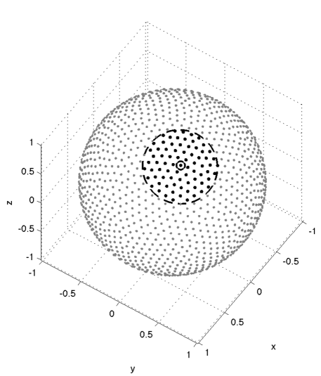
Figure 1: Illustration of the centers that make up the local Lagrange basis. The solid gray and black spheres mark the set of $N$ nodes making up $\Xi$. The solid black sphere with a circle around it marks the node $\xi$ where a local Lagrange function $\check{\chi}_{\xi}$ is to be computed. The the solid black spheres enclosed in the dashed circular line mark the set of $n=M(\log N)^{2}$ centers $\Upsilon(\xi)$ used to compute $\check{\chi}_{\xi}$. For each $\xi\in\Xi$, a similar set $\Upsilon(\xi)$ is determined for computing $\check{\chi}_{\xi}$.

The new basis for $S_{m}(\Xi)$ will consist of the collection of all the local Lagrange functions for the nodes in $\Xi$. It will be shown in Section 6.3 that by choosing the number of nearest neighbors to each $\xi$ as $n=M(\log N)^{2}$ will give a basis with sufficient locality. The choice of $M$ is related to the polynomial rate of decay of $\check{\chi}_{\xi}$ away from its center and a priori estimates are given for $M$ in Section 6.3. However, in practice it will be sufficient to choose $M$ by tuning it appropriately to get the desired rate of decay.

The exact details of the algorithm for constructing this basis then proceed as follows: For each $\xi\in\Xi$

1. Find the $n=M(\log N)^{2}$ nearest neighbors to $\xi$, $\Upsilon(\xi)$.

2. Construct $\check{\chi}_{\xi}$ according to the conditions (7), which amounts to solving the associated linear system (8) and storing the coefficients $\mathbf{A}_{\xi}$, ${\bf c}_{\xi}$.

We note each set $\Upsilon(\xi)$ can be determined in $\mathcal{O}(\log N)$ operations by using a KD-tree algorithm for sorting and searching through the nodes $\Xi$. After the initial construction of the KD-tree, which requires $\mathcal{O}(N(\log N)^{2})$, the construction of all the sets $\Upsilon(\xi)$ thus takes $\mathcal{O}(N(\log N)^{2})$ operations.

Before continuing, we note that our main results, given in Theorem 6.5 and its corollaries, depend heavily on properties that this local Lagrange basis inherits from the full Lagrange basis $\{\chi_{\xi}\}_{\xi\in\Xi}$. Thus, much of what follows is spent on developing a working understanding of the full Lagrange basis and its connections to the local Lagrange basis. Even though the local Lagrange basis is the focus of our work, we will delay any further mention of $\{\check{\chi}_{\xi}\}_{\xi\in\Xi}$ until Section 6.3.

4 The full Lagrange basis: numerical observations

In this section we numerically examine a full Lagrange basis function $\chi_{\xi}$ and its associated coefficients for the kernel $k_{2}(x,\alpha)=(1-x\cdot\alpha)\log(1-x\cdot\alpha)$, the second order restricted surface spline (also known as the thin plate spline) on $\mathbb{S}^{2}$. First, we demonstrate numerically that $\chi_{\xi}$ decays exponentially away from its center. Secondly, we provide the initial evidence that the Lagrange coefficients decay at roughly the same rate, which is proved later in Theorem 5.3.

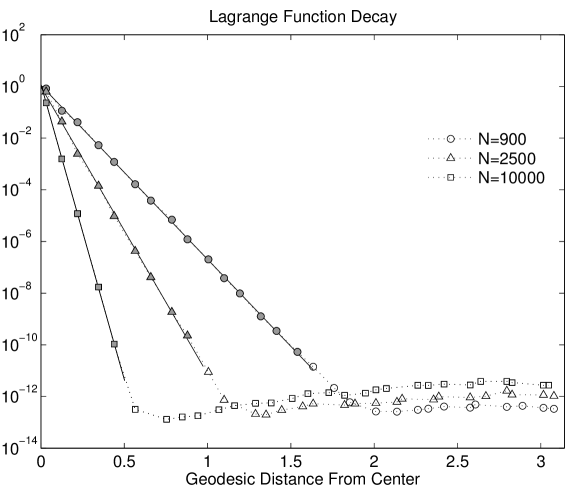
Figure 2: Maximum latitudinal values of the Lagrange function for the kernel $k_{2}(x,\alpha)$. This experiment was carried out in double precision arithmetic, and the plateau at roughly $10^{-11}$ occurs due to ill conditioning of the collocation matrices and truncation error.

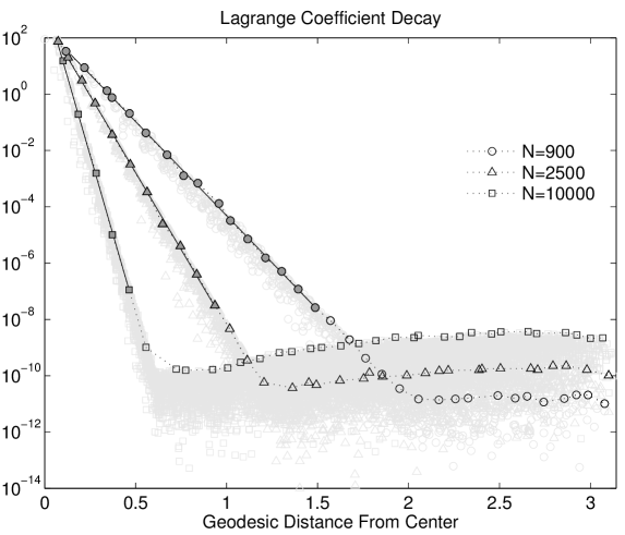
Figure 3: Plot of coefficients for a Lagrange function in the kernel space $S(k_{2},\Xi)$.This experiment was carried out in double precision arithmetic.

The full Lagrange function centered at $\xi$ takes the form

$$\chi_{\xi}=\sum_{\zeta\in\Xi}A_{\xi,\zeta}k(\cdot,\zeta)+p_{\xi},$$

where $p_{\xi}$ is a degree $1$ spherical harmonic. In this example, we use the “minimal energy points” of Womersley for the sphere – these are described and distributed at the website [25]. Because of the quasi-uniformity of the minimal energy point sets, it is sufficient to consider the Lagrange function $\chi_{\xi}$ centered at the north pole $\xi=(0,0,1)$.

Figure 2 displays the maximal colatitudinal values of $|\chi_{\xi}|$. Until a terminal value of roughly $10^{-11}$, we clearly observe the exponential decay of the Lagrange function, which follows

$$|\chi_{\xi}(x)|\leq C_{L}\exp\left(-\nu_{L}\frac{\mathrm{dist}(x,\xi)}{h}\right)$$ (9)

(this “plateau” at $10^{-11}$ is caused by roundoff error – see Figure 4). The estimate (9) has in fact been proven in [11, Theorem 5.3], where this and other analytic properties of bases for $S_{m}(\Xi)$ were studied in detail. By fitting a line to the data in Figure 2 where the exponential decay is evident, one can estimate the constants $\nu_{L}$ and $C_{L}$, which in this case are quite reasonable. For example, the value of $\nu_{L}$, which measures the rate of exponential decay, is observed to be close to $1.35$ (see Table 1).

We can visualize the decay of the corresponding coefficients in the same way. We again take the Lagrange function centered at the north pole: for each $\zeta^{\prime}\in\Xi$, the coefficient $|A_{\xi,\zeta^{\prime}}|$ in the expansion $\chi_{\xi}=\sum A_{\xi,\zeta}k(\cdot,\zeta)+p_{\xi}$ is plotted with horizontal coordinate $\text{dist}(\xi,\zeta^{\prime})$. The results for sets of centers of size $N=900,2500$ and $10000$ are given in Figure 3. The exponential decay seems to follow

$$|A_{\zeta,\xi}|\leq C_{c}q^{-2}\exp{\left(-\nu_{c}\frac{\mathrm{dist}(\xi,\zeta)}{h}\right)}.$$

Indeed, this is established later in Theorem 5.3. As before, we can estimate the constants $\nu_{c}$ and $C_{c}$ for the decay of the coefficients. Comparing Figures 2 and 3, we note that the coefficient plot is shifted vertically. This is a consequence of the factor of $q^{-2}$ in the estimate (15) below. Table 1 gives estimates for the constants $\nu_{c}$ and $C_{c}$, along with the constants involved in the decay of the Lagrange functions.

$N$	$h_{X}$	$\rho_{X}$	$\nu_{L}$	$C_{L}$	$\nu_{c}$	$C_{c}$
400	0.1136	1.2930	1.1119	0.8382	1.0997	0.5402
900	0.0874	1.5302	1.3556	1.0982	1.3445	0.7554
1600	0.0656	1.5333	1.3513	1.2170	1.3216	0.5946
2500	0.0522	1.5278	1.3345	0.9618	1.3117	0.5494
5041	0.0365	1.5304	1.3395	1.1080	1.3158	0.6188
10000	0.0260	1.5421	1.3645	1.1934	1.3369	0.7291

Table 1: Estimates of the decay constants $\nu$ and $C$ for Lagrange functions and coefficients on the sphere using the kernel $k_{2}(x,\alpha)$, with relevant geometric measurements of the minimum energy node sets used.

The perceived plateau present in the Lagrange function values as well as the coefficients shown in Figures 2 and 3 is due purely to round-off error related to the conditioning of kernel collocation and evaluation matrices. These results were produced using double-precision (approximately 16 digits) floating point arithmetic. To illustrate this point, we plot the decay rate of the Lagrange coefficients for the 900 and 1600 point node sets as computed using high-precision (40 digits) floating point arithmetic in Figure 4. The figure clearly shows that the exponential decay does not plateau, but continues as the theory predicts (see Theorem 5.3).

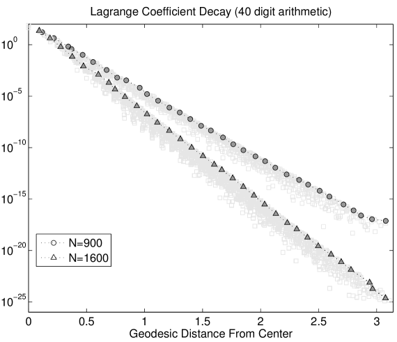
Figure 4: Size of the coefficients for a Lagrange function in the kernel space $S(k_{2},\Xi)$. This experiment was carried out in Maple with 40 digit arithmetic.

5 Coefficients of the full Lagrange functions

In this section we give theoretical results for the coefficients in the kernel expansion of Lagrange functions. In the first part we give a formula relating the size of coefficients to native space inner products of the Lagrange functions themselves (this is Proposition 5.1). We then obtain estimates for the restricted surface splines on $\mathbb{S}^{2}$, demonstrating the rapid, stationary decay of these coefficients.

5.1 Interpolation with conditionally positive definite kernels

In this section we demonstrate that the Lagrange function coefficients $A_{\xi,\zeta}$ can be expressed as a certain kind of inner product of different Lagrange functions $\chi_{\xi}$ and $\chi_{\zeta}$. Because this is a fundamental result, we work in generality in this subsection: the kernels we consider here are conditionally positive of the type considered in Section 2.2.

When $u,v\in S(k,\Xi)$ – meaning that they have the expansion $u=\sum_{\xi\in{\Xi}}a_{1,\xi}k(\cdot,\xi)+p_{u}$ and $v=\sum_{\xi\in{\Xi}}a_{2,\xi}k(\cdot,\xi)+p_{v}$ with coefficients $(a_{j,\xi})_{\xi\in\Xi}\perp(\varPi)|_{\Xi}$ for $j=1,2$ – then the semi-inner product is

$$\left\langle u,v\right\rangle_{k}=\left\langle\sum_{\xi\in{\Xi}}a_{1,\xi}k(\cdot,\xi),\sum_{\xi\in{\Xi}}a_{2,\xi}k(\cdot,\xi)\right\rangle_{k}=\sum_{\xi\in\Xi}\sum_{\zeta\in\Xi}a_{1,\xi}\overline{a_{2,\zeta}}k(\xi,\zeta).$$

(This follows directly from the definition (4) coupled with the observation that for $j\notin\mathcal{J}$, $\hat{u}(j)=\sum_{\xi\in{\Xi}}a_{1,\xi}\tilde{k}(j)\phi_{j}(\xi)$ and $\hat{v}(j)=\sum_{\xi\in{\Xi}}a_{2,\xi}\tilde{k}(j)\phi_{j}(\xi)$.) We can use this expression of the inner product to investigate the kernel expansion of the Lagrange function.

Proposition 5.1.

Let $k(\cdot,\xi)=\sum_{j\in\mathbb{N}}\tilde{k}(j)\phi_{j}(\cdot)\overline{\phi_{j}(\xi)}$ be a conditionally positive definite kernel with respect to the space $\varPi=\mathop{\mathrm{span}}_{j\in\mathcal{J}}\phi_{j}$, and let $\Xi$ be unisolvent for $\varPi$. Then $\chi_{\eta}\in S(k,\Xi)$ (the Lagrange function centered at $\eta$) has the kernel expansion $\chi_{\eta}(x)=\sum_{\xi\in\Xi}A_{\eta,\xi}k(x,\xi)+p_{\zeta}$ with coefficients

$$\mathbf{A}_{\eta}=(A_{\eta,\xi})_{\xi\in\Xi}=\bigl{(}\langle\chi_{\zeta}(x),\chi_{\eta}(x)\rangle_{k}\bigr{)}_{\xi\in\Xi}.$$

Proof.

Select two centers $\zeta,\eta\in\Xi$ with corresponding Lagrange functions $\chi_{\zeta}$ and $\chi_{\eta}\in S(k,\Xi)$. Denote the collocation and auxiliary matrices, introduced in Section 2.2, by $\mathrm{K}_{\Xi}=\bigl{(}k(\xi,\zeta)\bigr{)}_{\zeta,\xi}$ and $\Phi=\bigl{(}\phi_{j}(\xi)\bigr{)}_{\xi,j}$. Because $\mathbf{A}_{\zeta}$ and $\mathbf{A}_{\eta}$ are both orthogonal to $(\varPi)|_{\Xi}$, we have

$$\langle\chi_{\zeta},\chi_{\eta}\rangle_{k}=\sum_{\xi_{1}\in\Xi}\sum_{\xi_{2}\in\Xi}A_{\zeta,\xi_{1}}\overline{A_{\eta,\xi_{2}}}k(\xi_{1},\xi_{2})=\langle\mathrm{K}_{\Xi}\mathbf{A}_{\zeta},\mathbf{A}_{\eta}\rangle_{\ell_{2}(\Xi)}.$$

Now define $P:=\Phi(\Phi^{*}\Phi)^{-1}\Phi^{*}:\ell_{2}(\Xi)\to(\Pi_{\mathcal{J}})|_{\Xi}\subset\ell_{2}(\Xi)$ to be the orthogonal projection onto the subspace of samples of $\varPi$ on $\Xi$ and let $P^{\perp}=\mathrm{Id}-P$ be its complement. Then for any data ${\bf y}$, (3) yields coefficient vectors $\mathbf{A}$ and ${\bf c}$ satisfying $P^{\perp}\mathbf{A}=\mathbf{A}$ and $P^{\perp}\Phi{\bf c}={\bf 0}$, hence $P^{\perp}\mathrm{K}_{\Xi}P^{\perp}\mathbf{A}=P^{\perp}\mathrm{K}_{\Xi}\mathbf{A}=P^{\perp}{\bf y}$. Because $P^{\perp}:\ell_{2}(\Xi)\to\ell_{2}(\Xi)$ is also an orthogonal projector, and therefore self-adjoint, it follows that

$$\langle\chi_{\zeta}(x),\chi_{\eta}(x)\rangle_{k} = \langle\mathrm{K}_{\Xi}\mathbf{A}_{\zeta},\mathbf{A}_{\eta}\rangle_{\ell_{2}(\Xi)}$$

$$= \langle\mathrm{K}_{\Xi}\mathbf{A}_{\zeta},P^{\perp}\mathbf{A}_{\eta}\rangle_{\ell_{2}(\Xi)}$$

$$= \langle P^{\perp}\mathrm{K}_{\Xi}\mathbf{A}_{\zeta},\mathbf{A}_{\eta}\rangle_{\ell_{2}(\Xi)}$$

$$= \langle P^{\perp}{\bf e}_{\zeta},\mathbf{A}_{\eta}\rangle_{\ell_{2}(\Xi)}.$$

In the last line, we have introduced the sequence ${\bf e}_{\zeta}=(\delta_{\zeta,\xi})_{\xi\in\Xi}$ for which $\mathrm{K}_{\Xi}\mathbf{A}_{\zeta}+p_{\zeta}|_{\Xi}={\bf e}_{\zeta}$ which implies that $P^{\perp}\mathrm{K}_{\Xi}\mathbf{A}_{\zeta}=P^{\perp}{\bf e}_{\zeta}$. Using once more the fact that $P^{\perp}$ is self-adjoint, and that $\mathbf{A}_{\eta}$ is in its range, we have

$$\langle\chi_{\zeta}(x),\chi_{\eta}(x)\rangle_{k,\mathcal{J}}=\langle P^{\perp}{\bf e}_{\zeta},\mathbf{A}_{\eta}\rangle=\langle{\bf e}_{\zeta},P^{\perp}\mathbf{A}_{\eta}\rangle=\langle{\bf e}_{\zeta},\mathbf{A}_{\eta}\rangle$$

and the lemma follows. ∎

The next result involves estimating the norms $\|{\bf a}\|_{\ell_{2}(\Xi)}$ and $\|{\bf c}\|_{\ell_{2}(\mathcal{J})}$, where ${\bf a}$ and ${\bf c}$ are as in (3). It will be useful later, when we discuss local Lagrange functions. The notation is the same as that used in the proof above. In addition, because $k$ is a conditionally positive definite kernel for $\varPi$, the matrix $P^{\perp}\mathrm{K}_{\Xi}P^{\perp}$ is positive definite on the orthogonal complement of the range of $\Phi$. We will let $\vartheta$ be the minimum eigenvalue of this matrix; that is,

$$\vartheta:=\min_{\|P^{\perp}\alpha\|=1}\langle P^{\perp}\mathrm{K}_{\Xi}P^{\perp}\alpha,\alpha\rangle>0.$$

Proposition 5.2.

Suppose ${\bf a}$ and ${\bf c}$ satisfy (3). Let $G_{\Xi}=\Phi^{\ast}\Phi$. Then,

$$\|{\bf a}\|_{\ell_{2}(\Xi)}\leq\vartheta^{-1}\|{\bf y}\|_{\ell_{2}(\Xi)}\leq\vartheta^{-1}\sqrt{\#\Xi}\|{\bf y}\|_{\ell_{\infty}(\Xi)}$$

and

$$\|{\bf c}\|_{\ell_{2}(\mathcal{J})} \leq 2\|k\|_{\infty}\|G_{\Xi}^{-1}\|^{1/2}\vartheta^{-1}\#\Xi\|{\bf y}\|_{\ell_{2}(\Xi)}$$

$$\leq 2\|k\|_{\infty}\|G_{\Xi}^{-1}\|^{1/2}\vartheta^{-1}(\#\Xi)^{3/2}\|{\bf y}\|_{\ell_{\infty}(\Xi)}.$$

Proof.

From (3) and the fact that $P^{\perp}$ projects onto the orthogonal complement of the range of $\Phi$, we have that $P^{\perp}\mathrm{K}_{\Xi}P^{\perp}{\bf a}=P^{\perp}{\bf y}$ and that $P^{\perp}{\bf a}={\bf a}$. Consequently,

$$\vartheta\|{\bf a}\|_{\ell_{2}(\Xi)}^{2}=\vartheta\|P^{\perp}{\bf a}\|_{\ell_{2}(\Xi)}^{2}\leq\langle P^{\perp}\mathrm{K}_{\Xi}P^{\perp}{\bf a},{\bf a}\rangle\leq\|{\bf a}\|_{\ell_{2}(\Xi)}\|P^{\perp}{\bf y}\|_{\ell_{2}(\Xi)}.$$

The bound on $\|{\bf a}\|_{\ell_{2}(\Xi)}$ follows immediately from this and the estimate $\|{\bf y}\|_{\ell_{2}(\Xi)}\leq\sqrt{\#\Xi}\|{\bf y}\|_{\ell_{\infty}(\Xi)}$. To get the bound on $\|{\bf c}\|_{\ell_{2}(\Xi)}$, note that $\Phi{\bf c}=P{\bf y}-P\mathrm{K}_{\Xi}{\bf a}$ and, hence, that

$$\|\Phi{\bf c}\|_{\ell_{2}(\Xi)} \leq \|P{\bf y}\|_{\ell_{2}(\Xi)}+\|P\mathrm{K}_{\Xi}P^{\perp}{\bf a}\|_{\ell_{2}(\Xi)}$$

$$\leq \|P{\bf y}\|_{\ell_{2}(\Xi)}+\vartheta^{-1}\|P\mathrm{K}_{\Xi}P^{\perp}\|\|P^{\perp}{\bf y}\|_{\ell_{2}(\Xi)}$$

We also have that $\|\Phi{\bf c}\|_{\ell_{2}(\Xi)}^{2}=\langle\Phi^{\ast}\Phi{\bf c},{\bf c}\rangle\geq\lambda_{min}(\Phi^{\ast}\Phi)\|{\bf c}\|_{\ell_{2}(\mathcal{J})}^{2}$. However, $\lambda_{min}(\Phi^{\ast}\Phi)=\|(\Phi^{\ast}\Phi)^{-1}\|^{-1}$, which implies that

$$\|{\bf c}\|_{\ell_{2}(\mathcal{J})}\leq\|(\Phi^{\ast}\Phi)^{-1}\|^{1/2}\|\Phi{\bf c}\|_{\ell_{2}(\Xi)}=\|G_{\Xi}^{-1}\|^{1/2}\|\Phi{\bf c}\|_{\ell_{2}(\Xi)}$$

Next, note that the following inequalities hold: $\|P\mathrm{K}_{\Xi}P^{\perp}\|\leq\|\mathrm{K}_{\Xi}\|\leq\#\Xi\|k\|_{\infty}$, $\|P{\bf y}\|_{\ell_{2}(\Xi)},\|P^{\perp}{\bf y}\|_{\ell_{2}(\Xi)}\leq\|{\bf y}\|_{\ell_{2}(\Xi)}\leq\sqrt{\#\Xi}\|{\bf y}\|_{\ell_{\infty}(\Xi)}$, and $\frac{\#\Xi\|k\|_{\infty}}{\vartheta}\geq 1$. Applying these to the inequality

$$\|{\bf c}\|_{\ell_{2}(\mathcal{J})}\leq\|G_{\Xi}^{-1}\|^{1/2}\big{(}\|P{\bf y}\|_{\ell_{2}(\Xi)}+\#\Xi\|k\|_{\infty}\vartheta^{-1}\|P^{\perp}{\bf y}\|_{\ell_{2}(\Xi)}\big{)}$$

then yields the desired bound on $\|{\bf c}\|_{\ell_{2}(\mathcal{J})}$, completing the proof. ∎

5.2 Estimating Lagrange function coefficients

In [11], it has been shown that Lagrange functions for restricted surface splines decay exponentially fast away from the center. We can use these decay estimates in conjunction with Proposition 5.1 to estimate the decay of the coefficients $|A_{\xi,\zeta}|$.

Recall that the eigenvalues of $-\Delta$ are $\lambda_{\ell}=\ell(\ell+1)$. Let $Q(z):=\Pi_{\nu=1}^{m}(z-\lambda_{\nu-1})=\sum_{\nu=1}^{m}b_{\nu}z^{\nu}$. The kernel $k_{m}:\mathbb{S}^{2}\times\mathbb{S}^{2}\to\mathbb{R}$ has the expansion

$$k_{m}(x,\alpha)=\sum_{\ell=0}^{\infty}\tilde{k}(\ell)\sum_{\mu=-\ell}^{\ell}Y_{\ell}^{\mu}(x)Y_{\ell}^{\mu}(\alpha),$$

where, for $\ell\geq m$, $\tilde{k}(\ell)=C_{m}Q(\lambda_{\ell})^{-1}$, with $C_{m}=2^{m+1}\pi\Gamma(m)^{2}$ [17, Eqn. 3.3]. From the expansion, one sees that $k_{m}$ is conditionally positive definite with respect to $\Pi_{m-1}$. Kernels such as $k_{m}$ are said to be of polyharmonic or related type; they have been studied in [11]. The kernel $k_{m}$ acts as the Green’s function for the elliptic operator $\mathcal{L}_{m}:=C_{m}^{-1}Q(-\Delta)$ (cf. [11, Example 3.3]), in the sense that

$$f=\int_{\mathbb{M}}k_{m}(\cdot,\alpha)\mathcal{L}_{m}\bigl{[}f(\alpha)-p_{f}(\alpha)\bigr{]}\mathrm{d}\alpha+p_{f},$$

where $p_{f}$ is the orthogonal projection of $f$ onto $\Pi_{m-1}$.

The native space “inner product” on subsets. In [11] it was shown that for any $k\in\mathbb{N}$, the operator $(\nabla^{k})^{*}\nabla^{k}$ (which involves $(\nabla^{k})^{*}$ the adjoint – with respect to the $L_{2}(\mathbb{S}^{2})$ inner product – of the covariant derivative operator $\nabla^{k}$ which was introduced in Section 2.1) can be expressed as $\sum_{\nu=0}^{k}d_{\nu}\Delta^{\nu}$ with $d_{k}=(-1)^{k}$. Consequently, any operator of the form $\sum_{j=0}^{k}c_{j}(\nabla^{j})^{*}\nabla^{j}$ can be expressed as $\sum_{\nu=0}^{k}d_{\nu}\Delta^{\nu}$ with $d_{k}=(-1)^{k}c_{k}$ and vice-versa:

$$\forall(d_{0},\dots d_{m})\ \exists(c_{0},\dots,c_{m})\text{ with }d_{m}=(-1)^{m}c_{m}$$

$$\text{ and }\sum_{\nu=0}^{m}d_{\nu}\Delta^{\nu}=\sum_{j=1}^{m}c_{j}(\nabla^{j})^{*}\nabla^{j}.$$ (10)

Because $\mathcal{L}_{m}=C_{m}^{-1}Q(-\Delta)$, it follows that $\mathcal{L}_{m}=\sum_{j=0}^{m}c_{j}(\nabla^{j})^{*}\nabla^{j}$, with $c_{m}=C_{m}^{-1}$, and so the native space semi-inner product, introduced in (4), can be expressed as

$$\langle u,v\rangle_{k_{m}}=\langle\mathcal{L}_{m}u,v\rangle_{L_{2}(\mathbb{S}^{2})}=\int_{\mathbb{S}^{2}}\beta(u,v)_{x}\mathrm{d}\mu(x)$$

with $\beta(u,v)_{x}=\sum_{k=0}^{m}c_{k}\langle\nabla^{k}u,\nabla^{k}v\rangle_{x}$ and $c_{0},\dots,c_{m}$ are the appropriate constants guaranteed by (5.2). The latter expression allows us to extend naturally the native space inner product to measurable subsets $\Omega$ of $\mathbb{S}^{2}$. Namely,

$$\langle u,v\rangle_{\Omega,k_{m}}:=\int_{\Omega}\beta(u,v)_{x}\mathrm{d}\mu(x).$$

This has the desirable property of set additivity: for  sets $A$ and $B$ with $\mu(A\cap B)=0$, we have $\langle u,v\rangle_{A\cup B,k_{m}}=\langle u,v\rangle_{A,k_{m}}+\langle u,v\rangle_{B,k_{m}}.$ Unfortunately, since some of the coefficients $c_{k}$ may be negative, $\beta(u,u)$ and $\langle u,u\rangle_{\Omega,k_{m}}$ may assume negative values for some $u$: in other words, the bilinear form $(u,v)\mapsto\langle u,v\rangle_{\Omega,k_{m}}$ is only an indefinite inner product.

A Cauchy-Schwarz type inequality. When restricted to the cone of functions in $W_{2}^{m}(\Omega)$ having a sufficiently dense set of zeros, the quadratic form $\langle u,u\rangle_{\Omega,k_{m}}$ is positive definite. We now briefly discuss this.

When $\Omega$ has Lipschitz boundary and $u$ has many zeros, we can relate the quadratic form $\left|\!\left|\!\left|{u}\right|\!\right|\!\right|_{\Omega,k_{m}}^{2}:=\langle u,u\rangle_{\Omega,k_{m}}$ to a Sobolev norm $\|u\|_{W_{2}^{m}(\Omega)}^{2}$. Arguing as in [11, (4.2)], we see that

$$c_{m}|u|_{W_{2}^{m}(\Omega)}^{2} - \bigl{(}\max_{j\leq m-1}{|c_{j}|}\bigr{)}\|u\|_{W_{2}^{m-1}(\Omega)}^{2}$$

$$\leq \int_{\Omega}\beta(u,u)_{x}\mathrm{d}\mu(x)$$

$$\leq \bigl{(}\max_{j\leq m}{|c_{j}|}\bigr{)}\|u\|_{W_{2}^{m}(\Omega)}^{2}.$$

If $u|_{\Xi}=0$ on a set $\Xi$ with $h(\Xi,\Omega)\leq h_{0}$ with $h_{0}$ determined only by the boundary of $\Omega$ (specifically the radius and aperture of an interior cone condition satisfied by $\partial\Omega$), Theorem A.11 of [11] guarantees that $\|u\|_{W_{2}^{m-1}(\Omega)}^{2}\leq Ch^{2}|u|^{2}_{W_{2}^{m}(\Omega)}$ with $C$ depending only on the order $m$ and the roughness of the boundary (in this case, depending only on the aperture of the interior cone condition). Thus, by choosing $h\leq h^{*}$, where $h^{*}$ satisfies the two conditions

$$h^{*}\leq h_{0}\quad\text{and}\quad C(h^{*})^{2}\times\bigl{(}\max_{j\leq m}{|c_{j}|}\bigr{)}\leq\frac{|c_{m}|}{2},$$ (11)

we have

$$\frac{c_{m}}{2}\|u\|_{W_{2}^{m}(\Omega)}^{2}\leq\left|\!\left|\!\left|{u}\right|\!\right|\!\right|_{\Omega,k_{m}}^{2}\leq\left(\max_{j\leq m}|c_{j}|\right)\|u\|_{W_{2}^{m}(\Omega)}^{2}.$$

The threshold value $h^{*}$ depends on the coefficients $c_{j}$ as well as the radius $R_{\Omega}$ and aperture $\phi_{\Omega}$ of the cone condition for $\Omega$. When $\Omega$ is an annulus of sufficiently small inner radius, the cone parameters can be replaced by a single global constant, and $h_{*}$ can be taken to depend only on $c_{0},\dots,c_{m}$. In other words, only on $k_{m}$ – cf. [11, Corollary A.16].

A direct consequence of this is positive definiteness for such functions, $\left|\!\left|\!\left|{u}\right|\!\right|\!\right|_{\Omega,k_{m}}\geq 0$ with equality only if $u|_{\Omega}=0$. From this, we have a version of the Cauchy-Schwarz inequality: if $u$ and $v$ share a set of zeros $Z$ (i.e., $u|_{Z}=v|_{Z}=\{0\}$) that is sufficiently dense in $\Omega$, then

$$\left|\langle u,v\rangle_{\Omega,k_{m}}\right|\leq\left|\!\left|\!\left|{u}\right|\!\right|\!\right|_{\Omega,k_{m}}\left|\!\left|\!\left|{v}\right|\!\right|\!\right|_{\Omega,k_{m}}$$ (12)

follows (sufficient density means that $h(Z,\Omega)<h^{*}$ as above).

Decay of Lagrange functions. [11, Lemma 5.1] guarantees that the Lagrange function $\chi_{\xi}$ satisfies the bulk chasing estimate: there is a fixed constant $0\leq\epsilon<1$ so that for radii $r$ the estimate

$$\|\chi_{\xi}\|_{W_{2}^{m}(B^{c}(\xi,r))}\leq\epsilon\|\chi_{\xi}\|_{W_{2}^{m}(B^{c}(\xi,r-\frac{h}{4h_{0}}))}$$

holds. In other words, a fraction (roughly $1-\epsilon$) of the bulk of the tail $\|\chi_{\xi}\|_{W_{2}^{m}(B^{c}(\xi,r))}$ is to be found in the annulus $B(\xi,r)\setminus B(\xi,r-\frac{h}{4h_{0}})$ of width $\frac{h}{4h_{0}}\propto h$ (with a constant of proportionality $\frac{1}{4h_{0}}$ that depends only on $m$). For $r>0$, it is possible to iterate this $n$ times, provided $n\frac{h}{4h_{0}}\leq r$. It follows that there is $\nu=-4h_{0}\log\epsilon>0$ so that

$$\|\chi_{\xi}\|_{W_{2}^{m}(B^{c}(\xi,r))}\leq\epsilon^{n}\|\chi_{\xi}\|_{W_{2}^{m}(\mathbb{S}^{2})}\leq Ce^{-\nu r/h}\|\chi_{\xi}\|_{W_{2}^{m}(\mathbb{S}^{2})}.$$

By [11, (5.1)] we have

$$\|\chi_{\xi}\|_{W_{2}^{m}(B^{c}(\xi,r))}\leq Cq^{1-m}e^{-\nu\frac{r}{h}}.$$ (13)

This leads us to our main result.

Theorem 5.3.

Let $\rho>0$ be a fixed mesh ratio. There exist constants $h^{*}$, $\nu$ and $C$ depending only on $m$ and $\rho$ so that if $h\leq h^{*}$, then the Lagrange function $\chi_{\zeta}=\sum_{\xi\in\Xi}A_{\zeta,\xi}k_{m}(\cdot,\xi)+p_{\zeta}\in S_{m}(\Xi)$ has these properties:

$$|\chi_{\xi}| \leq C\exp\left(-\nu\frac{\mathrm{dist}(x,\xi)}{h}\right).$$ (14)

$$|A_{\zeta,\xi}| \leq Cq^{2-2m}\exp{\left(-\nu\frac{\mathrm{dist}(\xi,\zeta)}{h}\right)}.$$ (15)

$$c_{1}q^{2/p}\|{\bf a}\|_{\ell_{p}(\Xi)} \leq\big{\|}\sum_{\xi\in\Xi}a_{\xi}\chi_{\xi}\big{\|}_{L_{p}(\mathbb{S}^{2})}\leq c_{2}q^{2/p}\|{\bf a}\|_{\ell_{p}(\Xi)}.\quad$$ (16)

Proof.

The bounds (14) and (16) are given in [11, Theorems 5.3 & 5.7]. Only (15) requires proof. By Proposition 5.1 and set additivity, we have that

$$A_{\zeta,\xi}=\langle\chi_{\xi},\chi_{\zeta}\rangle_{k_{m}}=\langle\chi_{\xi},\chi_{\zeta}\rangle_{\Omega_{\zeta},k_{m}}+\langle\chi_{\xi},\chi_{\zeta}\rangle_{\Omega_{\xi},k_{m}},$$

where we employ the hemispheres: $\Omega_{\zeta}=\left\{\alpha\in\mathbb{S}^{2}\mid\mathrm{dist}(\alpha,\zeta)<\mathrm{dist}(\alpha,\xi)\right\},$ $\Omega_{\xi}=\left\{\alpha\in\mathbb{S}^{2}\mid\mathrm{dist}(\alpha,\xi)<\mathrm{dist}(\alpha,\zeta)\right\}.$ Modulo a set of measure zero, $\Omega_{\xi}=\mathbb{S}^{2}\setminus\Omega_{\zeta}$.

We apply the Cauchy–Schwarz type inequality (12) to obtain

$$|A_{\zeta,\xi}| \leq \left|\!\left|\!\left|{\chi_{\zeta}}\right|\!\right|\!\right|_{\Omega_{\zeta},k_{m}}\left|\!\left|\!\left|{\chi_{\xi}}\right|\!\right|\!\right|_{\Omega_{\zeta},k_{m}}+\left|\!\left|\!\left|{\chi_{\zeta}}\right|\!\right|\!\right|_{\Omega_{\xi},k_{m}}\left|\!\left|\!\left|{\chi_{\xi}}\right|\!\right|\!\right|_{\Omega_{\xi},k_{m}}$$

$$\leq \sqrt{\max_{j\leq m}|c_{j}|}\left(\|\chi_{\zeta}\|_{W_{2}^{m}(\Omega_{\zeta})}\left|\!\left|\!\left|{\chi_{\xi}}\right|\!\right|\!\right|_{\Omega_{\zeta},k_{m}}+\left|\!\left|\!\left|{\chi_{\zeta}}\right|\!\right|\!\right|_{\Omega_{\xi},k_{m}}\|\chi_{\xi}\|_{W_{2}^{m}(\Omega_{\xi})}\right)$$

Since $\Omega_{\zeta}\subset B^{c}(\zeta,r):=\mathbb{S}^{2}\setminus B\left(\zeta,\frac{1}{2}\mathrm{dist}(\xi,\zeta)\right)$ and $\Omega_{\xi}\subset B^{c}(\xi,r)$, we can again employ set additivity and positive definiteness (this time $\left|\!\left|\!\left|{\chi_{\xi}}\right|\!\right|\!\right|_{\Omega_{\zeta},k_{m}}\leq\left|\!\left|\!\left|{\chi_{\xi}}\right|\!\right|\!\right|_{\mathbb{S}^{2},k_{m}}$, which follows from the fact that $\mathbb{S}^{2}=\Omega_{\zeta}\cup\overline{\Omega_{\xi}}$ and that $\chi_{\xi}$ vanishes to high order in $\Omega_{\xi}$ – the same holds for $\chi_{\zeta}$) to obtain

$$|A_{\zeta,\xi}|\leq\sqrt{\max_{j\leq m}|c_{j}|}\left(\|\chi_{\zeta}\|_{W_{2}^{m}(B^{c}(\zeta,r))}\left|\!\left|\!\left|{\chi_{\xi}}\right|\!\right|\!\right|_{k_{m}}+\left|\!\left|\!\left|{\chi_{\zeta}}\right|\!\right|\!\right|_{k_{m}}\|\chi_{\xi}\|_{W_{2}^{m}(B^{c}(\xi,r))}\right).$$

The full energy of the Lagrange function can be bounded by comparing it to the energy of a bump function – for $\chi_{\xi}$ this is $\phi_{\xi}$, which can be defined by using a smooth cutoff function $\sigma$. In spherical coordinates (colatitude, longitude) around $\xi$, $\phi_{\xi}(\theta,\varphi)=\sigma(\theta/q).$ This is done in [11, (5.1)] and we have that $\left|\!\left|\!\left|{\chi_{\xi}}\right|\!\right|\!\right|_{k_{m}}$ and $\left|\!\left|\!\left|{\chi_{\zeta}}\right|\!\right|\!\right|_{k_{m}}$ are bounded by $Cq^{1-m}$.

On the other hand, we can employ (13) to treat $\|\chi_{\zeta}\|_{W_{2}^{m}(B^{c}(\zeta,r))}$ and $\|\chi_{\xi}\|_{W_{2}^{m}(B^{c}(\zeta,r))}$, which gives

$$\|\chi_{\xi}\|_{W_{2}^{m}(B^{c}\left(\zeta,r\right))},\|\chi_{\zeta}\|_{W_{2}^{m}(B^{c}\left(\zeta,r\right))}\leq Cq^{1-m}e^{-\nu\frac{r}{h}}=Cq^{1-m}e^{-\nu\frac{\mathrm{dist}(\xi,\zeta)}{2h}}.$$

The bound (15) follows immediately from this. ∎

Remark 5.4.

Because the proof doesn’t really depend on $\mathbb{S}^{2}$, a nearly identical proof works for any of the kernels with exponentially decaying Lagrange functions considered in [10, 11]. Specifically, we have this: Theorem 5.3 holds for compact, 2-point homogeneous spaces with polyharmonic kernels satisfying $\mathcal{L}_{m}\perp\Pi$ (cf. [11]) and for any compact, $C^{\infty}$ Riemannian manifold, with the kernels being the Sobolev splines given in [10].

6 Truncating the Lagrange basis

We now discuss truncating the kernel expansion Lagrange function $\chi_{\xi}=\sum_{\zeta\Xi}A_{\xi,\zeta}k_{m}(\cdot,\zeta)+p_{\xi}\in S_{m}(\Xi)$, replacing it with an expansion of the form

$$\widetilde{\chi}_{\xi}=\sum_{\zeta\in\Upsilon(\xi)}\widetilde{A}_{\xi,\zeta}k_{m}(\cdot,\zeta)+p_{\xi}\in S_{m}(\Xi),$$ (17)

where $\Upsilon(\xi)\subset\Xi$ is a set of centers contained in a ball $B(\xi,r(h))$ centered at $\xi$, where $r(h)$ and the $\widetilde{A}_{\xi,\zeta}$’s will be determined by $A_{\xi,\zeta}$, with $\zeta\in\Upsilon(\xi)$. We also assume that $\xi\in\Upsilon(\xi)$. Finally, to avoid notational clutter, we will simply use $\Upsilon$ rather than $\Upsilon(\xi)$.

Our goal is to show that if $\chi_{\xi}$ satisfies the properties (14), (15), and (16), then we may take $r(h)=Kh|\log(h)|$, with $K=K(m)>0$, while maintaining algebraic decay in $h$ of the error $\|\widetilde{\chi}_{\xi}-\chi_{\xi}\|_{\infty}$. For this choice of $r(h)$, a simple volume estimate (given at the end of Section 6.3) shows that the number of terms required for $\widetilde{\chi}_{\xi}$ is just $\mathcal{O}((\log N)^{2})\ll N$, far fewer than the $N$ needed for $\chi_{\xi}$.

Simply truncating at a fixed radius $r(h)=Kh|\log(h)|$ is not suitable, however, because the truncated function $\widetilde{\chi}_{\xi}$ will no longer be in the space $S_{m}(\Xi)$ (and thus $\{\widetilde{\chi}_{\xi}\}$ will not act as a basis). To treat this, we must slightly realign coefficients to satisfy the moment conditions.

A remark before proceeding with the analysis: Finding $\widetilde{\chi}_{\xi}$ in the way described below requires knowing the expansion for $\chi_{\xi}$ and carrying out the truncation above. This is expensive, although it does have utility in terms of speeding up evaluations for interpolation when the same set of centers is to be used repeatedly. The main point is that we now know roughly how many basis elements are required to obtain a good approximation to $\chi_{\xi}$. The question of producing a good basis efficiently is left to the next section.

6.1 Constraint conditions on the coefficients

We would like $\widetilde{\chi}_{\xi}$ to be in the space $S_{m}(\Xi)$, and so the $\widetilde{A}_{\xi,\zeta}$’s have to satisfy the constraints in the system (3):

$$\sum_{\zeta\in\Upsilon}\widetilde{A}_{\xi,\zeta}\overline{\phi_{j}}(\zeta)=0,\ j\in\mathcal{J}:=(1,\dots,m^{2}),$$ (18)

where $\{\phi_{j}\}_{j=1}^{m^{2}}$ is an orthonormal basis for $\Pi_{m-1}$. Since the original $\chi_{\xi}$’s are in $S_{m}(\Xi)$, the $A_{\xi,\zeta}$’s in their expansions satisfy the constraint equations in (3). Splitting these equations into sums over $\Upsilon$ and its complement in $\Xi$ and manipulating the result, we see that

$$\sum_{\zeta\in\Upsilon}A_{\xi,\zeta}\overline{\phi_{j}}(\zeta)+\sigma_{j},\quad\text{where }\sigma_{j}:=\sum_{\zeta\not\in\Upsilon}A_{\xi,\zeta}\overline{\phi_{j}}(\zeta),\ j\in\mathcal{J}.$$ (19)

The way that we will relate the two sets of coefficients is to define the vector $(\widetilde{A}_{\xi,\zeta})_{\zeta\in\Upsilon}$ to be the orthogonal projection of $(A_{\xi,\zeta})_{\zeta\in\Upsilon}$ onto the constraint space, which is the orthogonal complement of $\mathop{\mathrm{span}}\{\left.\phi_{j}\right|_{\Upsilon},j\leq m^{2}\}$, in the usual inner product for $\ell_{2}(\Upsilon)$. The equations below then follow:

$$(\widetilde{A}_{\xi,\zeta})_{\zeta\in\Upsilon}-(A_{\xi,\zeta})_{\zeta\in\Upsilon} =\sum_{j\in\mathcal{J}}\tau_{j}\phi_{j}|_{\Upsilon}\in\mathop{\mathrm{span}}\{(\phi_{j}(\zeta))_{\zeta\in\Upsilon},j\leq m^{2}\}$$ (20)

$$\|(\widetilde{A}_{\xi,\zeta})_{\zeta\in\Upsilon}-(A_{\xi,\zeta})_{\zeta\in\Upsilon}\|_{\ell_{2}(\Upsilon)}^{2} =\tau^{*}G_{\Upsilon}\tau,\ \ [G_{\Upsilon}]_{k,j}:=\textstyle{\sum_{\zeta\in\Upsilon}}\overline{\phi_{k}}(\zeta)\phi_{j}(\zeta),$$

where $\tau$ is a column vector having the $\tau_{j}$’s as entries. Let $\sigma$ be a column vector with the $\sigma_{j}$’s as entries. From the first equation above together with equations (18) and (19), $\tau$ and $\sigma$ are related by $\sigma=G_{\Upsilon}\tau$. If we make the rather mild assumption that $\Upsilon$ is unisolvent for the space $\Pi_{m-1}$, then we can invert $G_{\Upsilon}$: $\tau=G_{\Upsilon}^{-1}\sigma$, thereby obtaining $\tau^{*}G_{\Upsilon}\tau=\sigma^{*}G_{\Upsilon}^{-1}\sigma$. Using this in (20) and applying Schwarz’s inequality, we obtain this bound:

$$\big{\|}\textstyle{\sum_{\zeta\in\Upsilon}}(\widetilde{A}_{\xi,\zeta}-A_{\xi,\zeta})k_{m}(\cdot,\zeta)\big{\|}_{\infty}\leq\sqrt{\#\Upsilon\,\|G_{\Upsilon}^{-1}\|_{2}}\,\|k_{m}\|_{\infty}\|\sigma\|_{2},$$ (21)

which we will make use of to establish the estimates below.

Proposition 6.1.

Assume that $\Upsilon$ is unisolvent for $\Pi_{m-1}$ and that $\|G_{\Upsilon}^{-1}\|_{2}=\mathcal{O}(|\log h|^{-2}\,h^{-2\mu})$, for some $\mu\geq 0$. If we take $r(h)=Kh|\log(h)|$, where $K$ is chosen so that $J:=K\nu-2m-\mu>0$ then for $h$ sufficiently small,

$$\|\widetilde{\chi}_{\xi}-\chi_{\xi}\|_{\infty}\leq Ch^{J}$$ (22)

$$|\widetilde{\chi}_{\xi}(x)|\leq C\big{(}1+\mathrm{dist}(x,\xi)/h\big{)}^{-J}$$ (23)

Furthermore, when $J>2$, the set $\{\widetilde{\chi}_{\xi}\}$ is $L_{p}$ stable: there are $C_{1},C_{2}>0$ for which

$$C_{1}q^{2/p}\|{\bf a}\|_{\ell_{p}(\Xi)}\leq\big{\|}\textstyle{\sum_{\xi\in\Xi}}a_{\xi}\widetilde{\chi}_{\xi}\big{\|}_{L_{p}(\mathbb{S}^{2})}\leq C_{2}q^{2/p}\|{\bf a}\|_{\ell_{p}(\Xi)}.$$ (24)

Proof.

From (15) and $N\leq 4\pi/\mathrm{vol}(B(\xi,q))\leq Cq^{-2}$, we have that

$$\sum_{\zeta\not\in\Upsilon}|A_{\xi,\zeta}|=\mathcal{O}\big{(}Nq^{2-2m}\exp(-\nu r(h)/h)\big{)}\leq Ch^{K\nu-2m}.$$ (25)

Applying it to the $\sigma_{j}$’s defined in (19) results in $\|\sigma\|_{2}\leq Ch^{K\nu-2m}$. Using this in connection with (21), $\|G_{\Upsilon}^{-1}\|_{2}=\mathcal{O}(|\log h|^{-2}\,h^{-2\mu})$, (25) and

$$\widetilde{\chi}_{\xi}-\chi_{\xi}=\sum_{\zeta\in\Upsilon}(\widetilde{A}_{\xi,\zeta}-A_{\xi,\zeta})k_{m}(\cdot,\zeta)-\textstyle{\sum_{\zeta\not\in\Upsilon}}A_{\xi,\zeta}k_{m}(\cdot,\zeta),$$

yields (22). Next, from (14) we have

$$|\chi_{\xi}| \leq C\exp\left(-\nu\frac{\mathrm{dist}(x,\xi)}{h}\right)$$

$$\leq C\exp\left(-K\nu\frac{\mathrm{dist}(x,\xi)}{Kh}\right)$$

$$\leq C\bigg{(}1+\frac{\mathrm{dist}(x,\xi)}{Kh}\bigg{)}^{-K\nu}.$$

Combining this with (22), using $J=K\nu-2m-\mu>0$ and manipulating, we arrive at (23).

It remains to demonstrate the $L_{p}$ stability of $(\tilde{\chi}_{\xi})$ for $1\leq p\leq\infty$. When $p=1$, we consider a sequence ${\bf a}=(a_{\xi})_{\xi\in\Xi}\in\ell_{1}(\Xi)$. Let $s:=\sum a_{\xi}\chi_{\xi}$ and $\tilde{s}:=\sum a_{\xi}\widetilde{\chi}_{\xi}$. From Hölder’s inequality and (22), we have $\|\tilde{s}-s\|_{L_{1}(\mathbb{S}^{2})}\leq C\|{\bf a}\|_{\ell_{1}(\Xi)}h^{J}$ and

$$\|\tilde{s}-s\|_{L_{\infty}(\mathbb{S}^{2})}\leq C\|{\bf a}\|_{\ell_{\infty}(\Xi)}\underbrace{\textstyle{\sum_{\xi\in\Xi}}|\widetilde{\chi}_{\xi}(x)-\chi_{\xi}(x)|}_{\leq N\max_{\xi}\|\widetilde{\chi}_{\xi}-\chi_{\xi}\|_{L_{\infty}(\mathbb{S}^{2})}}\leq C\|{\bf a}\|_{\ell_{\infty}(\Xi)}h^{J}q^{-2}.$$

Interpolating between these two inequalities – i.e., interpolating the finite rank operator ${\bf a}\mapsto(s-\tilde{s})$ – gives

$$\|s-\tilde{s}\|_{L_{p}(\mathbb{S}^{2})} \leq Ch^{J}q^{-2(1-1/p)}\|{\bf a}\|_{\ell_{p}(\Xi)}$$

$$\leq Ch^{J-2}q^{2/p}\|{\bf a}\|_{\ell_{p}(\Xi)}.\quad(q^{-2}\sim h^{-2}).$$

After some manipulation, this bound and (16) imply that

$$c_{1}q^{2/p}\|{\bf a}\|_{\ell_{p}(\Xi)}(1-Ch^{J-2})\leq\|\tilde{s}\|_{L_{p}(\mathbb{S}^{2})}\leq c_{2}q^{2/p}\|a\|_{\ell_{p}(\Xi)}(1+Ch^{J-2}).$$

Choosing $h$ so that $Ch^{J-2}\leq 1/2$ and letting $C_{1}=c_{1}/2$ and $C_{2}=3c_{2}/2$, we obtain (24). ∎

Remark 6.2.

When there are no constraint conditions on the coefficients, this result holds for any of the strictly positive definite kernels mentioned in Remark 5.4. In particular it holds for Sobolev splines on a compact $C^{\infty}$ Riemannian manifold.

6.2 Norm of the inverse Gram matrix

We now demonstrate that the conditions on $G_{\Upsilon}^{-1}$ in Proposition 6.1 are automatically satisfied. We will state and prove the results below for caps on $\mathbb{S}^{d}$, rather than just $\mathbb{S}^{2}$. Also, It is more convenient to use with $\Pi_{L}$ rather than $\Pi_{m-1}$, because $m$ is notationally tied to the polyharmonic kernels $k_{m}$ as well as the spherical harmonics on $\mathbb{S}^{2}$. That said, we begin with the lemma below.

Lemma 6.3.

Suppose that $S_{r}:=B(\xi,r)\subset\mathbb{S}^{d}$ is a cap of fixed radius $r<\pi$, and that ${\mathscr{C}}\subset S_{r}$ is finite and has mesh norm $h_{\mathscr{C}}:=h_{S_{r},{\mathscr{C}}}$. In addition, let $L\geq 0$ be a fixed integer and take $\Pi_{L}$ to be the space of all spherical harmonics of degree at most $L$. Then, there exists a constant $c_{0}:=c_{0}(d,L)>0$ such that when $h_{\mathscr{C}}\leq c_{0}r$ we have

$$\sum_{\zeta\in{\mathscr{C}}}|\varphi(\zeta)|^{2}\geq\mu(S_{r})^{-1}\int_{S_{r}}|\varphi(x)|^{2}d\mu(x),\ \text{for all }\varphi\in\Pi_{L}.$$ (26)

Moreover, the set ${\mathscr{C}}$ is unisolvent for $\Pi_{L}$. Finally, for every basis for $\Pi_{L}$ the corresponding Gram matrices $G_{\mathscr{C}}$ and $G_{S_{r}}$, relative to the inner products on $\ell^{2}({\mathscr{C}})$ and $S_{r}$, respectively, satisfy

$$\|G_{\mathscr{C}}^{-1}\|_{2}\leq\mu(S_{r})\|G_{S_{r}}^{-1}\|_{2}.$$ (27)

Proof.

Since since $\varphi(x)$ and $\overline{\varphi}(x)$ are spherical harmonics in $\Pi_{L}$, their product is a spherical harmonic of degree at most $2L$. Thus, applying the nonnegative-weight quadrature formula in [16, Theorem 2.1] to spherical harmonics of order $2L$ yields

$$\sum_{\zeta\in{\mathscr{C}}}w_{\zeta}|\varphi(\zeta)|^{2}=\int_{S_{r}}|\varphi(x)|^{2}d\mu(x),$$

Since $0\leq w_{\zeta}\leq\sum_{\zeta\in{\mathscr{C}}}w_{\zeta}=\mu(S_{r})$, we have the inequality $\sum_{\zeta\in{\mathscr{C}}}w_{\zeta}|\varphi(\zeta)|^{2}\leq\mu(S_{r})\sum_{\zeta\in{\mathcal{C}}}|\varphi(\zeta)|^{2}$. The inequality (26) follows immediately from the quadrature formula. To prove that ${\mathcal{C}}$ is unisolvent, suppose that $\varphi\in\Pi_{L}$ vanishes on ${\mathcal{C}}$. By (26), we have that $\int_{S_{r}}|\varphi(x)|^{2}d\mu(x)=0$. Since $\varphi$ is in $\Pi_{L}$, it is a polynomial in sines and cosines of the angles used in the standard parameterization of $\mathbb{S}^{d}$, with $\xi$ being the “north” pole. As a consequence, it is continuous on $S_{r}$ and, because $\int_{S_{r}}|\varphi(x)|^{2}d\mu(x)=0$, it is identically $0$ on $S_{r}$. Finally, as a function of the angular variables in the complex plane, it is analytic, entire in fact, and can be expanded in a power series in these variables. The fact that it vanishes identically for real values of the angular variables is enough to show that the coefficients in the series are all zero. Hence, $\varphi\equiv 0$ on $\mathbb{S}^{d}$ and ${\mathscr{C}}$ is unisolvent for $\Pi_{L}$. To establish (27), note that (26) implies that $G_{\mathscr{C}}-\mu(S_{r})^{-1}G_{S_{r}}$ is positive semi definite. From the Courant-Fischer theorem, the lowest eigenvalue of $G_{\mathscr{C}}$ is greater than that of $\mu(S_{r})^{-1}G_{S_{r}}$. This inequality then yields (27), since these eigenvalues are $\|G_{\mathscr{C}}^{-1}\|_{2}^{-1}$ and $\mu(S_{r})\|G_{S_{r}}^{-1}\|_{2}^{-1}$, respectively. ∎

We now need to compute the Gram matrix for the canonical basis of $\Pi_{L}$. This basis is described in [24, Chapter IX, §3.6] and consists of spherical harmonics. Let $\ell,k_{1},\ldots,k_{d-1}$ be integers satisfying $\ell\geq k_{1}\geq k_{2}\geq\cdots\geq k_{d-1}\geq 0$, and take $K:=(k_{1},\ldots,\pm k_{d-1})$. A spherical harmonic of degree $\ell$ [24, p. 466]) will be denoted by $Y^{\ell}_{K}(\theta_{1},\ldots,\theta_{d})$. The angles are the usual ones from spherical coordinates in $\mathbb{R}^{d+1}$ (cf. [24, p. 435]). The basis for $\Pi_{L}$ is then the set of all $Y^{\ell}_{K}$, $0\leq\ell\leq L$. The entries in the Gram matrix are $[G_{S_{r}}]_{(\ell,K),(\ell^{\prime},K^{\prime})}=\langle Y^{\ell}_{K},Y^{\ell^{\prime}}_{K^{\prime}}\rangle_{S_{r}}$. Following the argument in [24, Chapter IX, §3.6], one may show that

$$\langle Y^{\ell}_{K},Y^{\ell^{\prime}}_{K^{\prime}}\rangle_{S_{r}}\\ =B_{\ell,K}B_{\ell^{\prime},K}\delta_{K,K^{\prime}}\int_{0}^{r}C^{\frac{d-1}{2}+k_{1}}_{\ell-k_{1}}(\cos\theta)C^{\frac{d-1}{2}+k_{1}}_{\ell^{\prime}-k_{1}}(\cos\theta)\sin^{2k_{1}+d-1}\theta d\theta,$$ (28)

where $C^{s}_{n}(t)$ is the Gegenbauer polynomial of degree $n$ and type $s$, and $B_{\ell,k_{1}}$ is a normalization factor. In the case where $d=2$ and $L=1$, $G_{S_{r}}$ is $4\times 4$ and has six non-zero entries,

$$\begin{array}[]{rrcl}&G_{(0,0),(0,0)}&=&\frac{1}{2}(1-\cos r),\\ &G_{(0,0),(1,0)}=G_{(1,0),(0,0)}&=&\frac{\sqrt{3}}{4}(1-\cos r)(1+\cos r),\\ &G_{(1,0),(1,0)}&=&\frac{1}{2}(1-\cos r)(1+\cos r+\cos^{2}r),\\ &G_{(1,\pm 1),(1,\pm 1)}&=&\frac{1}{4}(1-\cos r)^{2}(2+\cos r).\end{array}$$

Since $\mu(S_{r})=2\pi(1-\cos r)$, the formulas for the entries above imply that $G_{S_{r}}/\mu(S_{r})$ is a polynomial in $\cos r$. In fact, a straightforward calculation shows that the minimum eigenvalue of this matrix is $r^{4}/(256\pi)+\mathcal{O}(r^{6})$. Lemma 6.3 then implies that $\|G_{\mathcal{C}}^{-1}\|_{2}\leq\mu(S_{r})\|G_{S_{r}}^{-1}\|_{2}=256\pi r^{-4}+\mathcal{O}(r^{-2})$. A less precise, but similar result, holds in the general case.

Lemma 6.4.

Under the assumptions of Lemma 6.3, for general $L\geq 0$, $d\geq 2$ and $r$ sufficiently small, there is an integer $\iota=\iota(L,d)\geq L$ and a constant $C=C(L,d)>0$ such that $\|G_{\mathcal{C}}^{-1}\|_{2}\leq Cr^{-2\iota}$. For $L=1$ and $d=2$, we may take $\iota=2$.

Proof.

From the expression in (28) for the entries in $G_{S_{r}}$, we see that each of them is entire in $r$ and has a zero of order $d$ or greater at $r=0$. In addition, $\mu(S_{r})$ is also entire in $r$ and has a zero of order $d$. It follows that the matrix $\widetilde{G}(r)=G_{S_{r}}/\mu(S_{r})$ is entire, even in $r$. and for real $r$, it is real, self adjoint and positive semi definite. (In fact, for $d$ even, it is a polynomial in $\cos r$.) In addition, the $2\times 2$ block in $\widetilde{G}(0)$ corresponding to $k_{1}=0$, $\ell=0,1$, is rank 1 and therefore has 0 as an eigenvalue; consequently, $\widetilde{G}(0)$ also has 0 as an eigenvalue – it’s lowest, in fact. As Rellich [19, pg. 91] shows, the eigenvalues of $\widetilde{G}(r)$ are analytic functions of $r$. For $r>0$, these eigenvalues are proportional to those of the Gram matrix $G_{S_{r}}$ and therefore must be positive. None of these eigenvalues are identically $0$. In particular, the eigenvalues splitting off from the $0$ eigenvalue of $\widetilde{G}(0)$ are not identically $0$. As functions of $r$ they thus have a zero of finite order at $r=0$; the order is an even integer because $\widetilde{G}(r)$ is even in $r$. The smallest eigenvalue then behaves like $\lambda_{min}(r)=r^{2\iota}(a_{0}+\mathcal{O}(r^{2}))$, where $a_{0}>0$, $\iota>0$ is an integer, and $r$ is sufficiently small. Furthermore, from (28) we see that the diagonal entry, with $\ell=\ell^{\prime}=k_{1}=L$, is $\mathcal{O}(r^{2L})$. since this bounds the minimum eigenvalue from above, we must have $2\iota\geq 2L$, so $\iota\geq L$. The result then follows from Lemma 6.3 and the observation that $\mu(S_{r})\|G_{S_{r}}^{-1}\|_{2}=\lambda_{min}^{-1}$. The calculation for $L=1$ and $d=2$ was done above. ∎

6.3 Local Lagrange Bases

We now turn to the local Lagrange basis. Recall that the function $\check{\chi}_{\xi}\in S_{m}(\Xi)$, with the kernel representation

$$\check{\chi}_{\xi}=\sum_{\zeta\in\Upsilon}\check{A}_{\xi,\zeta}k_{m}(\cdot,\zeta)+\sum_{j=1}^{m^{2}}\check{b}_{j}\phi_{j}\in S_{m}(\Xi),$$ (29)

is a local Lagrange function centered at $\xi$ if it satisfies $\check{\chi}_{\xi}|_{\Upsilon}={\bf e}_{\xi}$, where ${\bf e}_{\xi}(\zeta)=\delta_{\xi,\zeta}$; that is, ${\bf e}_{\xi}$ is the vector $(1,0,\ldots,0)^{T}$. Since $\check{\chi}_{\xi}\in S_{m}(\Xi)$, the vector $\check{A}_{\xi}=(\check{A}_{\xi,\zeta})_{\zeta\in\Upsilon}$ is in the constraint space. This vector and the coefficients $\check{b}_{j}$ then satisfy $\check{\chi}_{\xi}|_{\Upsilon}={\bf e}_{\xi}$, Of course, the (full) Lagrange function $\chi_{\xi}=\sum_{\zeta\in\Xi}A_{\xi,\zeta}\kappa(\cdot,\zeta)+\sum_{j=1}^{m^{2}}b_{j}\phi_{j}$ restricted to $\Upsilon$ also satisfies $\chi_{\xi}|_{\Upsilon}={\bf e}_{\xi}$. Consequently, $\mathfrak{D}_{\xi}:=\check{\chi}_{\xi}-\chi_{\xi}$ satisfies $\mathfrak{D}_{\xi}|_{\Upsilon}=\bf 0$. We can rewrite this difference as $\mathfrak{D}_{\xi}=\check{\chi}_{\xi}-\widetilde{\chi}_{\xi}+\widetilde{\chi}_{\xi}-\chi_{\xi}$ (with $\widetilde{\chi}_{\xi}$ the truncated basis function introduced in the last section). It follows that

$$\mathfrak{D}_{\xi}=\underbrace{\sum_{\zeta\in\Upsilon}(\underbrace{\check{A}_{\zeta}-\widetilde{A}_{\zeta}}_{\displaystyle{\alpha_{\zeta}}})\kappa(\cdot,\zeta)+\sum_{j=1}^{\#\mathcal{J}}(\underbrace{\check{b}_{j}-b_{j}}_{\displaystyle{\beta_{j}}})\phi_{j}}_{\check{\chi}_{\xi}-\widetilde{\chi}_{\xi}}+\widetilde{\chi}_{\xi}-\chi_{\xi}.$$

Evaluating this on $\Upsilon$ then gives the system $\mathrm{K}_{\Upsilon}\alpha+\Phi\beta+(\widetilde{\chi}_{\xi}-\chi_{\xi})|_{\Upsilon}=\bf 0$. By linearity, it is clear that $\Phi^{\ast}\alpha=\bf 0$. Finally, letting ${\bf y}=(\chi_{\xi}-\widetilde{\chi}_{\xi})|_{\Upsilon}$, we arrive at the system,

$$\begin{pmatrix}\mathrm{K}_{\Upsilon}&\Phi\\ \Phi^{*}&\bf 0\end{pmatrix}\begin{pmatrix}\alpha\\ \beta\end{pmatrix}=\begin{pmatrix}{\bf y}\\ {\bf 0}\end{pmatrix}.$$ (30)

Proposition 5.2 applies to (30), with $\Xi$ replaced by $\Upsilon$; thus, noting that $\|{\bf y}\|_{\ell_{\infty}(\Upsilon)}\leq\|\widetilde{\chi}_{\xi}-\chi_{\xi}\|_{\infty}$, and writing $\mathcal{J}=(1,\dots,m^{2})$, we see that

$$\|\alpha\|_{\ell_{2}(\Upsilon)}\leq\vartheta^{-1}\sqrt{\#\Upsilon}\|\widetilde{\chi}_{\xi}-\chi_{\xi}\|_{\infty}$$

$$\|\beta\|_{\ell_{2}(\mathcal{J})}\leq 2\|k_{m}\|_{\infty}\|G_{\Upsilon}^{-1}\|^{1/2}\vartheta^{-1}(\#\Upsilon)^{3/2}\|\widetilde{\chi}_{\xi}-\chi_{\xi}\|_{\infty}$$

From this we obtain these inequalities:

$$\|\check{\chi}_{\xi}-\widetilde{\chi}_{\xi}\|_{\infty} \leq\|k_{m}\|_{\infty}\sqrt{\#\Upsilon}\|\alpha\|_{\ell_{2}(\Upsilon)}+mC_{m}\|\beta\|_{\ell_{2}(\mathcal{J})},\ C_{m}=\max_{j\leq m^{2}}\|\phi_{j}\|_{\infty}$$

$$\leq\|k_{m}\|_{\infty}\#\Upsilon\vartheta^{-1}\bigg{(}1+2mC_{m}\sqrt{\#\Upsilon\|G_{\Upsilon}^{-1}\|}\bigg{)}\|\widetilde{\chi}_{\xi}-\chi_{\xi}\|_{\infty}$$

Moreover, using $\|\check{\chi}_{\xi}-\chi_{\xi}\|_{\infty}\leq\|\check{\chi}_{\xi}-\widetilde{\chi}_{\xi}\|_{\infty}+\|\chi_{\xi}-\widetilde{\chi}_{\xi}\|_{\infty}$, we see that

$$\|\check{\chi}_{\xi}-\chi_{\xi}\|_{\infty}\leq 2\|k_{m}\|_{\infty}\#\Upsilon\vartheta^{-1}\bigg{(}1+2mC_{m}\sqrt{\#\Upsilon\|G_{\Upsilon}^{-1}\|}\bigg{)}\|\widetilde{\chi}_{\xi}-\chi_{\xi}\|_{\infty}.$$ (31)

Finally, from Proposition 6.1, if $K>(2m+2\mu)/\nu$, it is easy to see that this holds:

$$\|\check{\chi}_{\xi}-\chi_{\xi}\|_{\infty}\leq C\frac{|\log h|^{2}}{\vartheta}\left(1+mh^{-\mu}\right)h^{K\nu-2m-\mu}\leq C\frac{|\log h|^{2}}{\vartheta}h^{K\nu-2m-2\mu}.$$ (32)

To proceed further, we need to estimate $\vartheta$. Such estimates are known for surface splines in the Euclidean case [18, §6]. Simply repeating the proofs of [18, Corollary 2.2] and [18, Theorem 2.4] for a set of points in $\mathbb{R}^{3}$ restricted to $\mathbb{S}^{2}$ yields the desired estimate. For the collocation matrix associated with $k_{m}$ and $\Xi$, we have

$$\vartheta\geq Cq^{2m-2},$$ (33)

where $C$ depends only on $m$. Thus, for $k_{m}$, we have $\|\check{\chi}_{\xi}-\chi_{\xi}\|_{\infty}\leq Ch^{K\nu-4m+2-2\mu}$, where the constant $K$ has to be increased slightly to absorb $|\log h|^{2}$. With this in mind we have the following result, whose proof, being similar to Proposition  6.1, we omit.

Theorem 6.5.

Let the notation and assumptions of Theorem 5.3 hold. Suppose that $K>0$ is chosen so that $K>\frac{4m-2+2\mu}{\nu}$ and, for each $\xi\in\Xi$, $\Upsilon(\xi):=\Xi\cap B(\xi,Kh|\log h|)$. If $\check{\chi}_{\xi}$ is a local Lagrange function for $\Upsilon(\xi)$ centered at $\xi$, then set $\{\check{\chi}_{\xi}\}_{\xi\in\Xi}$ is a basis for $S_{m}(\Xi)$. Moreover, with $J:=K\nu-4m+2-2\mu$, we have

$$\|\check{\chi}_{\xi}-\chi_{\xi}\|_{\infty}\leq C\ h^{J},$$ (34)

$$|\check{\chi}_{\xi}(x)|\leq C\big{(}1+\mathrm{dist}(x,\xi)/h\big{)}^{-J}.$$ (35)

Furthermore, when $J>d$, the set $\{\check{\chi}_{\xi}\}$ is $L_{p}$ stable: there are $C_{1},C_{2}>0$ for which

$$C_{1}q^{2/p}\|{\bf a}\|_{\ell_{p}(\Xi)}\leq\big{\|}\textstyle{\sum_{\xi\in\Xi}}a_{\xi}\check{\chi}_{\xi}\big{\|}_{L_{p}(\mathbb{S}^{2})}\leq C_{2}q^{2/p}\|{\bf a}\|_{\ell_{p}(\Xi)}.$$ (36)

Quasi-interpolation: It follows that the operator

$$Q_{\Xi}f=\sum_{\xi\in\Xi}f(\xi)\check{\chi}_{\xi}$$

provides $L_{\infty}$ convergence at the same asymptotic rate as interpolation $I_{\Xi}$. Indeed,

$$|I_{\Xi}f(x)-Q_{\Xi}f(x)|\leq\sum_{\xi\in\Xi}|\check{\chi}_{\xi}(x)-\chi_{\xi}(x)||f(\xi)| \leq Cq^{-2}\|f\|_{\infty}{h}^{K\nu-4m-2\mu}$$

$$\leq C\|f\|_{\infty}h^{2m}$$

provided that $K>\frac{6m+2\mu+2}{\nu}.$ It is shown in [11, Corollary 5.9] that restricted surface spline interpolation exhibits $\|I_{\Xi}f-f\|_{\infty}\leq Ch^{\sigma}$ for $f\in C^{2m}(\mathbb{S}^{2})$ when $\sigma=2m$ and for $f\in B_{\infty,\infty}^{\sigma}(\mathbb{S}^{2})$ for $\sigma<2m$. So $Q_{\Xi}$ has the same rate of approximation (without needing to solve a large system of equations).

Constructing basis functions in terms of $N$. Given a set of scattered points, it may be desirable to use $N$ as the basic parameter instead of $h$. Therefore we wish to express the number of nearest neighbors needed as a function of the total cardinality $N$ instead of those within a $Kh\log h$ neighborhood. Considering a cap $B(\alpha,r)$, a simple volume argument gives

$$\#(B(\alpha,r)\cap\Xi)\leq\frac{36}{11}\left(\frac{r}{q}\right)^{2}.$$ (37)

Indeed, one arrives at this bound by first considering caps of radius $q$ around each node in $B(\alpha,r)$. If $q$ is small enough, say $q<r$, then at least $1/3$ the volume of each cap will be contained in $B(\alpha,r)$. Using this and a Taylor expansion of the volume formula $2\pi(1-\cos(q))$ leads to (37). Thus, the greatest number of points in a cap of radius $Kh|\log h|$ is $\frac{36}{11}\rho^{2}\bigl{(}K\log(1/h)\bigr{)}^{2}$. Also, it is not hard to show that $2h^{-2}\leq N,$ and hence it follows that the number of points is bounded by $\frac{36}{11}\rho^{2}\bigl{(}\frac{K}{2}\log(N)\bigr{)}^{2}=\frac{9}{11}(\rho K)^{2}\bigl{(}\log(N)\bigr{)}^{2}$, and it suffices to take for $\Upsilon$ the nearest $\frac{9}{11}(\rho K)^{2}\bigl{(}\log(N)\bigr{)}^{2}$ neighbors.

The constants $\nu$ and $K$. Before we turn to a discussion of preconditioning, we wish to comment on the constants $\nu$ and $K$ above. These two constants come into play in a crucial way in many of our estimates.

The decay constant $\nu$ first comes up in the proof of Theorem 5.3. (Although we do not mention it in the theorem, the proof produces two different decay constants: $\nu_{L}$ and $\nu_{C}$, the former for the Lagrange function and the latter for the coefficients.) The estimate for $\nu$ is, of course, a lower bound on the decay constant itself; it is independent of $\rho$, but weakly dependent on $m$. Because of the nature of such estimates, it is very likely that they are much lower than $\nu_{\text{actual}}$. How $\nu_{\text{actual}}$ behaves as a function of $\rho$ is an open question.

There is another open question concerning $K$. We know that it must be bounded below by $\frac{4m-2+2\mu}{\nu}$. Thus a better estimate on $\nu$ would produce a better lower bound on $K$. This in turn means using smaller caps and fewer points in constructing the local Lagrange interpolant – i.e., giving it a smaller “footprint.” On the other hand, the larger we make $K$ the better the approximation to $\chi_{\xi}$ we get. Since $K$ can be made as large as we please, the question then becomes this: What is an optimal choice for $K$? Indeed, what does the term optimal mean here?

7 Preconditioning with local Lagrange functions

In this section we illustrate how the local Lagrange functions can also be used as an effective preconditioner for linear systems associated with interpolation using the standard restricted spline basis. Our focus is on the restricted surface spline $k_{2}$ (i.e. the restricted thin plate spline), for which the interpolant to $f\bigr{|}_{\Xi}$ in the standard basis takes the form

$$I_{\Xi}f=\sum_{\xi\in\Xi}a_{\xi}k_{2}(\cdot,\xi)+\sum_{j=1}^{4}c_{j}\phi_{j}(\cdot),$$ (38)

where $\phi_{j}$ are a basis for the spherical harmonics of degree $\leq 1$. We note that this interpolant can also be written with respect to the local Lagrange basis for $S_{2}(\Xi)$ as

$$I_{\Xi}f=\sum_{\xi\in\Xi}{\check{a}}_{\xi}\check{\chi}_{\xi}(\cdot);$$ (39)

see Section 3 for the details on constructing this basis.

Using the properties of the local Lagrange basis, we can write the linear system for determining the interpolation coefficients ${\check{a}}_{\xi}$ in (39) as:

$$\begin{bmatrix}\mathrm{K}_{\Xi}&\Phi\end{bmatrix}\begin{bmatrix}\mathsf{A}_{\Upsilon}\\ \mathsf{C}_{\Upsilon}\end{bmatrix}\begin{bmatrix}\mathbf{\check{a}}\end{bmatrix}=\begin{bmatrix}\mathbf{f}\end{bmatrix},$$ (40)

where $(\mathrm{K}_{\Xi})_{i,j}=k_{2}(\xi_{i},\xi_{j})$, $i,j=1,\ldots,N$, and $\Phi_{i,j}=\phi_{j}(\xi_{i})$, $i=1,\ldots,N$, $j=1,\ldots,4$. The matrix $\mathsf{A}_{\Upsilon}$ is a $N$-by-$N$ sparse matrix where each column contains $n=M(\log N)^{2}$ entries corresponding to the values of the interpolation coefficients $A_{\xi,\zeta}$ for the local Lagrange basis in (6). The matrix $\mathsf{C}_{\Upsilon}$ is a $4$-by-$N$ matrix with each column containing the values of the interpolation coefficients $c_{\xi,j}$ in (6). With the linear system written in this way, one can view the matrix $[\mathsf{A}_{\Upsilon}\;\mathsf{C}_{\Upsilon}]^{T}$ as a right preconditioner for the standard kernel interpolation matrix. Once $\mathbf{\check{a}}$ is determined from (40), we can then find the interpolation coefficients $a_{\xi}$ and $c_{j}$ in (38) from

$$[\mathbf{a}\;\mathbf{c}]^{T}=[\mathsf{A}_{\Upsilon}\;\mathsf{C}_{\Upsilon}]^{T}\mathbf{a}.$$ (41)

If the local Lagrange basis decays sufficiently fast then the linear system (40) should be “numerically nice” in the sense that the matrix $\mathrm{K}_{\Xi}\mathsf{A}_{\Upsilon}+\Phi\mathsf{C}_{\Upsilon}$ should have decaying elements from its diagonal and should be well conditioned. As discussed in the previous section, the decay is controlled by the number of nearest neighbors $n$ used in constructing each local Lagrange function and that $n=M(\log N)^{2}$. In the experiments below, we found that choosing $n=7\lceil(\log N)^{2}/(\log 10)^{2})\rceil=7\lceil(\log_{10}N)^{2}\rceil$ gave very good results over several decades of $N$.

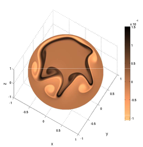
Figure 5: Interpolated relative vorticity from a numerical simulation of the shallow water wave equations on the $N=163842$ icosahedral node sets. The original values for the relative vorticity come from [8] and have been interpolated to a regular $300\times 600$ latitude-longitude based grid using the restricted kernel spline $k_{2}(x,\alpha)=(1-x\cdot\alpha)\log(1-x\cdot\alpha)$. The interpolation coefficients were computed using GMRES on the preconditioned system (40).

To solve the preconditioned linear system (40) we will use the generalized minimum residual method (GMRES) [21]. This is a Krylov subspace method which is applicable to non-symmetric linear systems and only requires computing matrix-vector products. Each matrix-vector product involving the preconditioner matrix $[A_{\Upsilon}\;\mathsf{C}_{\Upsilon}]^{T}$ requires $\mathcal{O}\bigl{(}N(\log N)^{2}\bigr{)}$ operations, while each matrix-vector product involving $[\mathrm{K}_{\Xi}\;\Phi]$ requires $\mathcal{O}(N^{2})$ operations. However, Keiner et al. have shown that this latter product can be done in $\mathcal{O}(N\log N)$ operations using fast algorithms for spherical Fourier transforms [13]. As we are primarily interested in the exploring the effectiveness of the local Lagrange basis as a preconditioner, we have not used these fast algorithms in the results below. In a follow up study, we will investigate these fast algorithms in combination with the preconditioner in much more detail.

For the first numerical tests we use icosahedral node sets $\Xi\subset\mathbb{S}^{2}$ of increasing cardinality. These were chosen because of their popularity in computational geosciences (see, for example, [9, 22, 20, 15]) where interpolation between node sets is often required. The values of $f$ were chosen to take on random values from a uniform distribution between $[-1,1]$. Table 2 displays the number of GMRES iterations to compute an approximate solution to the resulting linear systems (40) for various $N$ and different tolerances. As we can see, the number of iterations is small and stays relatively constant as $N$ increases.

		Number GMRES iterations
$N$	$n$	$tol=10^{-6}$	$tol=10^{-8}$
2562	84	7	5
10242	119	5	7
23042	140	6	7
40962	154	5	7
92162	175	6	8
163842	196	5	7

Table 2: Number of GMRES iterations required for computing an approximate solution to (40) using icosahedral node sets of cardinality $N$. Here $n$ corresponds to the number of nodes used to construct the local basis and $tol$ refers to the tolerance on the relative residual in the GMRES method. The right hand side was set to random values uniformly distributed between $[-1,1]$ and the initial guess for GMRES was set equal to the function values.

For the final numerical experiment, we use the above technique to interpolate a field taken from a numerical simulation on the icosahedral node sets to a regular latitude-longitude grid. As mentioned above, this is often necessary for purposes of comparing solutions from different computational models, plotting solutions, or coupling different models together. The data we use comes from [8] and represents the relative vorticity of a fluid described by the shallow water wave equations on the surface of a rotating sphere. The initial conditions for the model lead to the development of a highly nonlinear wave with rapid energy transfer from large to small scales, resulting in complex vortical dynamics. The numerical solution was computed on the $N=163842$ node set and we interpolated it to a regular $300\times 600$ latitude-longitude based grid. Figure 5 displays the resulting interpolated relative vorticity from the simulation at time $t=6$ days. The figure clearly shows that the complex flow structure has been maintained after the interpolation. As in the numerical examples above, the approximate solution to (40) with this data was obtained in 7 iterations of the GMRES method using a tolerance of $10^{-8}$.

References

• [1] R. Beatson and L. Greengard, A short course on fast multipole methods, in Wavelets, multilevel methods and elliptic PDEs (Leicester, 1996), Numer. Math. Sci. Comput., Oxford Univ. Press, New York, 1997, pp. 1–37.
• [2] R. K. Beatson, J. B. Cherrie, and C. T. Mouat, Fast fitting of radial basis functions: methods based on preconditioned GMRES iteration, Adv. Comput. Math., 11 (1999), pp. 253–270. Radial basis functions and their applications.
• [3] R. K. Beatson and M. J. D. Powell, An iterative method for thin plate spline interpolation that employs approximations to Lagrange functions, in Numerical analysis 1993 (Dundee, 1993), vol. 303 of Pitman Res. Notes Math. Ser., Longman Sci. Tech., Harlow, 1994, pp. 17–39.
• [4] R. K. Beatson, M. J. D. Powell, and A. M. Tan, Fast evaluation of polyharmonic splines in three dimensions, IMA J. Numer. Anal., 27 (2007), pp. 427–450.
• [5] G. E. Fasshauer, Meshfree approximation methods with MATLAB, vol. 6 of Interdisciplinary Mathematical Sciences, World Scientific Publishing Co. Pte. Ltd., Hackensack, NJ, 2007. With 1 CD-ROM (Windows, Macintosh and UNIX).
• [6] A. C. Faul, G. Goodsell, and M. J. D. Powell, A Krylov subspace algorithm for multiquadric interpolation in many dimensions, IMA J. Numer. Anal., 25 (2005), pp. 1–24.
• [7] A. C. Faul and M. J. D. Powell, Proof of convergence of an iterative technique for thin plate spline interpolation in two dimensions, Adv. Comput. Math., 11 (1999), pp. 183–192. Radial basis functions and their applications.
• [8] N. Flyer, E. Lehto, S. Blaise, G. B. Wright, and A. St-Cyr, A guide to RBF-generated finite differences for nonlinear transport: shallow water simulations on a sphere, J. Comput. Phys., 231 (2012), pp. 4078–4095.
• [9] F. X. Giraldo, Lagrange-Galerkin methods on spherical geodesic grids, J. Comput. Phys., 136 (1997), pp. 197–213.
• [10] T. Hangelbroek, F. J. Narcowich, and J. D. Ward, Kernel approximation on manifolds I: Bounding the Lebesgue constant, SIAM Journal on Mathematical Analysis, 42 (2010), pp. 1732–1760.
• [11] T. Hangelbroek, F. J. Narcowich, and J. D. Ward, Polyharmonic and related kernels on manifolds: Interpolation and approximation, Foundations of Computational Mathematics, (2012), pp. 1–46. 10.1007/s10208-011-9113-5.
• [12] M. J. Johnson, A symmetric collocation method with fast evaluation, IMA J. Numer. Anal., 29 (2009), pp. 773–789.
• [13] J. Keiner, S. Kunis, and D. Potts, Fast summation of radial functions on the sphere, Computing, 78 (2006), pp. 1–15.
• [14] L. Ling and E. J. Kansa, A least-squares preconditioner for radial basis functions collocation methods, Adv. Comput. Math., 23 (2005), pp. 31–54.
• [15] D. Majewski, D. Liermann, P. Prohl, B. Ritter, M. Buchhold, T. Hanisch, G. Paul, W. Wergen, and J. Baumgardner, The operational global icosahedral-hexagonal gridpoint model GME: Description and high-resolution tests, Mon. Wea. Rev., 130 (2002), pp. 319–338.
• [16] H. N. Mhaskar, Local quadrature formulas on the sphere, J. Complexity, 20 (2004), pp. 753–772.
• [17] H. N. Mhaskar, F. J. Narcowich, J. Prestin, and J. D. Ward, $L^{p}$ Bernstein estimates and approximation by spherical basis functions, Math. Comp., 79 (2010), pp. 1647–1679.
• [18] F. J. Narcowich and J. D. Ward, Norm estimates for the inverses of a general class of scattered-data radial-function interpolation matrices, J. Approx. Theory, 69 (1992), pp. 84–109.
• [19] F. Rellich, Perturbation theory of eigenvalue problems, Assisted by J. Berkowitz. With a preface by Jacob T. Schwartz, Gordon and Breach Science Publishers, New York, 1969.
• [20] T. D. Ringler, R. P. Heikes, and D. A. Randall, Modeling the atmospheric general circulation using a spherical geodesic grid: A new class of dynamical cores, Mon. Wea. Rev., 128 (2000), pp. 2471–2490.
• [21] Y. Saad and M. H. Schultz, GMRES: A generalized minimal residual algorithm for solving nonsymmetric linear systems, SIAM J. Sci. Comput., 7 (1986), pp. 856–869.
• [22] G. R. Stuhne and W. R. Peltier, New icosahedral grid-point discretizations of the shallow water equations on the sphere, J. Comput. Phys., 148 (1999), pp. 23–53.
• [23] T. Tran, Q. T. Le Gia, I. H. Sloan, and E. P. Stephan, Preconditioners for pseudodifferential equations on the sphere with radial basis functions, Numer. Math., 115 (2010), pp. 141–163.
• [24] N. J. Vilenkin, Special functions and the theory of group representations, Translated from the Russian by V. N. Singh. Translations of Mathematical Monographs, Vol. 22, American Mathematical Society, Providence, R. I., 1968.
• [25] R. Womersley, Minimum energy points on the sphere $\mathbb{S}^{2}$. http://web.maths.unsw.edu.au/~rsw/Sphere/Energy/index.html, 2003.