Capacity and Spectral Efficiency of Interference Avoiding Cognitive Radio with Imperfect Detection
Abstract
In this paper, we consider a model in which the unlicensed or the Secondary User (SU) equipped with a Cognitive Radio (CR) (together referred to as CR) interweaves its transmission with that of the licensed or the Primary User (PU). In this model, when the CR detects the PU to be (i) busy it does not transmit and; (ii) PU to be idle it transmits. Two situations based on CR’s detection of PU are considered, where the CR detects PU (i) perfectly - referred to as the “ideal case” and; (ii) imperfectly - referred to as “non ideal case”. For both the cases we bring out the rate region, sum capacity of PU and CR and spectral efficiency factor - the ratio of sum capacity of PU and CR to the capacity of PU without CR. We consider the Rayleigh fading channel to provide insight to our results. For the ideal case we study the effect of PU occupancy on spectral efficiency factor. For the non ideal case, in addition to the effect of occupancy, we study the effect of false alarm and missed detection on the rate region and spectral efficiency factor. We characterize the set of values of false alarm and missed detection probabilities for which the system benefits, in the form of admissible regions. We show that false alarm has a more profound effect on the spectral efficiency factor than missed detection. We also show that when PU occupancy is small, the effects of both false alarm and missed detection decrease. Finally, for the standard detection techniques viz. energy detection, matched filter and magnitude squared coherence, we show that that the matched filter performs best followed by magnitude squared coherence followed by energy detection with respect to spectral efficiency factor.
I Introduction
While certain parts of the frequency spectrum are crowded by users, most part of the spectrum still remains heavily unoccupied [1]. Due to this spectrum imbalance, the legacy command and control policy of the FCC and the recent proliferation in usage of wireless devices, new techniques that can perform Dynamic Spectrum Access (DSA) are needed. The so called Cognitive Radio (CR), in essence, performs DSA by sensing the radio environment, choosing the best channel (frequency, time slot or codes) that is available and adapting parameters to communicate simultaneously ensuring the interference to legacy users below a prescribed level [2].
In literature (for example [3], [4]) there are three paradigms for CR based systems mentioned, based upon the nature of operation of the CR, viz. (i) interference avoiding or interweave, (ii) interference limited or underlay and (iii) interference mitigating or overlay. Each of the above paradigm assumes different amounts or levels of side information that the SU has about PU transmission.
From an information theoretic viewpoint, most of the recent works focus on modelling the CR channel as an interference channel with some side information about the PU codebooks, messages, channel characteristics etc, being available to the CR transmitter [4]-[15]. Also they mostly address underlay and overlay based CRNs.
In [5] a two switch model for CR is presented with one switch at the SU transmitter and the other at the SU receiver. The role of each switch is to identify transmitting opportunity (channel) which can be different at the SUs transmitter and receiver. Transmission is then done on a channel which is identified to be free on both the transmitter and the receiver ends. In [6] the CR channel is modeled as two sender two receiver model with the transmitters having non causal information. In [7],[8] capacity for low and high interference regimes is analyzed, wherein the PU codeword is assumed to be known to the CR. Extending from two user case to the three user case, in [9] achievable rate regions and outer bounds are derived. Channels are modeled as interference channels where the transmitters cooperate in a unidirectional manner via 3 different noncausal message-sharing mechanism specified therein.
For the case of underlay based systems, in [10],[11] the capacity gains offered when only partial channel information of the link between the CR transmitter and PU receiver is available to the CR under average received power constraint is studied. In [12] an optimal power allocation policy to maximize capacity, which exploits a two-dimensional frequency-selectivity on CRs own channel as well as CR to PU channel under an interference-power constraint as well as a conventional transmit power constraint is proposed. Moving further ahead [13] proposes a joint overlay and underlay technique to maximize the total capacity of CR.
While most of the above works either attempt to characterize the achievable regions or maximize CR capacity, certain works study about the sum capacity of the CR and PU together so that capacity gains of entire system is brought out [14],[15].
Significantly, all the above works assume that the CR and PU have perfect side information about the PU occupancy. Although such models are of use, practical scenarios wherein there is imperfect side information available needs to be studied as capacity can decrease with imperfect side information, significantly.
In [3], a simple rate region involving rates of PU and CR has been brought out for the case where the CR interweaves its communication with the PU by means of time sharing. It is assumed therein that CR has perfect knowledge of PU’s channel occupancy. We refer to this as the “ideal case”.
In this paper, we find the spectral efficiency factor, which is the ratio of the sum capacity of CR and PU to the capacity of the PU in absence of CR, for the ideal case. With the help of an example of Rayleigh flat fading channel, we study its variation with PU occupancy for different relative power levels of the CR and PU. Along with the ideal case, we consider the case where CR interweaves its communication with PU with “only an imperfect” knowledge of the PUs channel occupancy. We refer to this as the “non ideal case”. We obtain rate regions for the non ideal case and compare it with the ideal case. We show that the rate region of the non ideal case is a sub-region of the ideal case. We also discuss the effects of false alarm and missed detection on the rate region for the non ideal case. We then find the maximum sum capacity and use this expression compute the spectral efficiency factor. We bring out effects of false alarm and missed detection on the spectral efficiency factor. We show that, probability of false alarm has more profound effect than the missed detection on spectral efficiency factor.
In the ideal case the, spectral efficiency factor is always greater than unity. However, in the non ideal case, if the error in detection is large, i.e. the probability of false alarm, , and the probability of missed detection, , either individually or collectively transgress certain limits; the spectral efficiency factor turns out to be less than unity. We characterize regions made up of those points, called the admissible regions, for which we obtain spectral efficiency factor greater than unity. Finally we compare known detection schemes from a spectral efficiency perspective.
The rest of the paper is as follows. In Section II we discuss the system model. In Section III we show the rate region for the case where the CR detects the PU perfectly. We then address the non ideal detection and characterize the corresponding rate region in Section IV. We also find conditions for obtaining maximum sum capacity therein. Then we discuss the spectral efficiency factor in Section V, wherein we discuss the effects of false alarm and missed detection on the spectral efficiency factor. We then show a comparison of the certain standard detection techniques in light of the results obtained in section VI. Finally conclusions are given in section VII.
II System Model
In this paper we assume that the Primary User (PU) transmits with a probability and the channel is free with a probability . However, from a detection perspective, the occupancy of a single channel is defined as the unconditional probability that the measured signal strength does exceeds some predetermined threshold [16]. In spectrum sensing, the detection involves comparing a test statistic against a threshold, suitably chosen. Let be the observed random variable and the transmit random variable, so that if there is no transmission and 0 otherwise. It follows that . We now discuss the system models for the two cases based on the relation of and .
II-A System Model for Ideal Detection
In case of perfect detection, . This is referred to as the case of “ideal” detection. The system model is described in Fig. 1.
The baseband relations for the PU and the CR are defined as
| (1) |
where and are the signals transmitted, and are the signals received by the PU and the CR respectively. and are uncorrelated circularly symmetric zero mean variance white Gaussian random variables i.i.d. over time for the PU and CR respectively, denoted as, . The average power constraints on the PU and CR are and . The fading coefficients and are uncorrelated and i.i.d over time. These channels are asymmetrically time shared, i.e. the CR channel comes into existence only when the PU channel is not used.
II-B System Model for Non Ideal Detection
In general, , which is referred to as the case of “non ideal” detection. In non ideal detection there are errors in detection. The probability of false alarm, is the probability that CR detects the channel to be free given it was occupied by the PU. Similarly, the probability of missed detection, , is the probability that CR detects the channel to be occupied given it was free from PU transmission [17]. Note that the other two conditional probabilities can be expressed in terms of and . The system model for non ideal case is as shown in Fig. 2.
Due to the possibility of false alarm, the PU and CR might transmit at the same time, which leads to a possibility of the interference channel. Hence, the channel can be a pure flat fading channel with probability and an interference channel with probability . The entire channel is time shared between a pure flat fading channel for PU, a pure flat fading channel for the CR and finally an interference channel for the PU and CR. We thus have a time sharing random variable as follows.
Definition 1.
Time sharing random variable is as defined
-
1.
is the event that , CR correctly detects the channel to be free;
-
2.
is the event that , CR erroneously detects the channel to be free;
-
3.
is the event that , CR erroneously detects the channel to be occupied;
-
4.
is the event that , CR correctly detects the channel to be occupied.
The probability distribution on is as follows
| (2) |
Note that respectively denote the instances where there is a flat fading channel for the CR, an interference channel between the PU and the CR, and a flat fading channel for the PU. Also note that is the instance where the channel goes waste as there is no transmission during this time, neither from PU nor from CR. The distribution of the time sharing random variable is fixed for a given . We have the baseband representation as
| (3) |
where , , , , , , and remain the same as in the ideal case. and are also i.i.d over time and uncorrelated with each other as well as with and .
The system model for the non ideal case is a very general model and encompasses some of the models available. In Fig. 3, we have shown how the two switch model proposed in [5] can be expressed as a special case of the model we have proposed. There are three possibilities, viz (i) the CR transmitter and the receiver detect the same channels to be free. Here the CR transmitts using perfect knowledge and this is the case of ideal detection i.e. , (ii) the CR tranmsitter finds certain channels to be free which are not found free at the CR receiver hence if the CR transmits then it interfers with the PU which implies , and (iii) the CR receiver determines free channels but the CR transmitter does not which leads to a loss in transmission opportunity an hence, .
III Rate Region and Spectral Efficiency Factor for Ideal Detection
In this section we present the rate region [3] and spectral efficiency factor for ideal detection. These results help in presenting the non ideal case in proper perspective. We then define spectral efficiency factor as the ratio of the sum capacity of the CR and PU to the capacity of PU in absence of CR. We discuss its variation as a function of for different values of relative transmit power levels of CR and PU with help of an example.
The system model for the ideal case is described in subsection II-A. The average capacity for the PU, , and CR, , is given by [18]
| (4) |
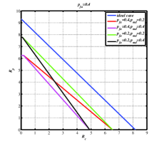
The corresponding rate region is given by
| (5) |
where the rates of the PU transceiver pair and of the CR transceiver pair is achieved through ideal white space filling [3]. Fig. 4 shows the rate region.
The sum capacity of PU and CR is . There are three possible cases viz. (i) , in this case maximizes the sum capacity, (ii) , in this case maximizes the sum capacity, and (iii) , in this case any value of would maximize the sum capacity.
We now define spectral efficiency factor in terms of the sum capacity as
Definition 2.
Spectral efficiency factor, , is defined as the ratio of sum capacity of CR and PU to the capacity of PU in the absence of CR. Formally,
where,
-
•
= PUs data rate achievable with CR present,
-
•
= CRs achievable data rate
-
•
= PUs data rate achievable without CR present.
With this definition, we have
Theorem 1.
The Spectral efficiency factor for ideal detection with average power constraints as and for the CR and PU respectively is given by
where and are as given in (III).
The value of this factor is always greater than unity as the CR transmits when the primary is idle, making more use of resource. It is of interest to see the variation of with .
Corollary 1.
increases with with a rate of .
Proof.
As increases, then decreases which implies that increases. Hence increases with . Since and are independent of , increases with . By differentiating w.r.t. , we get the slope of the curve of . ∎
We look at an example where fading is Rayleigh to better understand the consequence of Corollary 1.
Example 1.
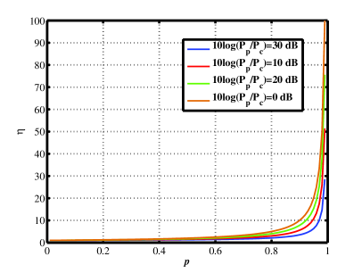
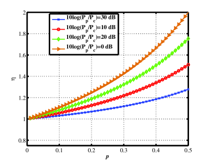
Consider, the fading coefficients and to be uncorrelated and i.i.d over time, circularly symmetric zero mean complex Gaussian random variables with unit variance, denoted as . Thus are Rayleigh distributed with parameter value 1, denoted as . We assume a fixed mW and we take 4 different values of such that dB. We make plot of the vs for these 4 different cases. Note that throughout the paper has the same definition unless otherwise specified.
We observe from Fig. 5, that for higher values of , increases rapidly irrespective of . This is clear from Corollary 1 since increases rapidly, faster than increase in and does not effect . Hence, even if increases slightly increases rapidly. Looking at Fig. 5, for dB, when we move from to , the spectral efficiency factor increases from 5 to around 50 which is a ten times increase. Comparing this to dB, the growth is more rapid from to there is 20 times increase. Hence, for higher the growth is more rapid. To study the effect of for small value of , i.e. we blow up a portion of Fig. 4 in Fig. 5. Observe when is less, irrespective of , the growth rate of is much higher than the case when is higher. This is evident from Corollary 1 since lower would imply higher .
Note that while for the ideal case is greater than unity, in the non ideal case it may not always be greater than unity as we see in the Section V.
Note that all the Figs. 8 - 10 and 13-22 are plotted for Rayleigh fading channels with unit second moment. That is all , , and are complex Gaussian random variables with zero mean and unit variance. However, since we consider average or ergodic capacity, the analysis and conclusions are valid for any other distribution for which expectation is finite. Also note that the average received SNR at the PU receiver is assumed to be unless otherwise specifically mentioned.
IV Rate Region and maximum sum capacity for Non Ideal Detection
In this section, we find out the rate region for the non ideal case for which the system model is discussed in section II-B. By considering all the cases defined in the time sharing random variable in definition 1, we bring out the capacity expressions and then specify the rate region. We look at the effects of , and together on the rate region with the help of plots. We see that the rate region approaches that of the ideal case as tend to zero. We then write the sum capacity and maximize it under two specific type of constraints viz, when is specified and the maximization is over . The other case is when are specified and maximization is over .
We have,
Lemma 1.
The average capacity and of the PU and CR for average transmit power constraints and are respectively as follows
| (6) | ||||
| (7) |
where,
The units are again bits/complex dimensions.
Proof.
We consider the 4 different situations described by .
-
•
For we have the baseband equations as given in (II-B) and reproduced here,
Hence, the capacity of CR given is
Note that .
-
•
For we have the baseband equations as given in (II-B) and reproduced here,
Here, both the PU and CR treat each others transmissions as Gaussian noise with mean 0 and variance and respectively. Hence, the total noise variance for the PU and CR is and respectively. Hence, capacity of the PU and CR is
-
•
For . We have .
-
•
For we have the baseband equations as given in equation (II-B)
Hence, the capacity of PU given is
Note that .
Finally we have, the capacity for CR and PU as
| (8) | ||||
| (9) |
These follow from the distribution of the time sharing random variable defined in the system model in subsection II-B. ∎
Note that the values of , , and as specified in the Lemma 1, will be used throughout the paper unless otherwise specified.
The corresponding rate region is given by
| (10) |
where the rates, of the PU transceiver pair and of the CR transceiver pair are achieved through non ideal white space filling. Also, , and . Note that,
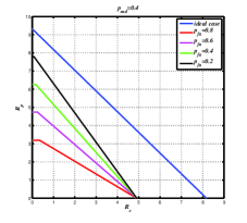
where is the rate region of the ideal case, specified in 5. In other words, as tends to zero. This implies that for smaller values of , the rate region in the non ideal case comes closer to that of the ideal case. Consider the rate region shown in Fig. 7, the interior of the red diagonal line along with the axes, specifies the rate region of the ideal detection and interior of the blue line along with the axes, specifies the rate region for the non ideal detection. Clearly, the non ideal case is the sub-region of the ideal case as it completely lies inside the ideal case region. Moreover, the cut on the vertical (or PU) axis, given by , is purely due to , while that on the horizontal (or CR) axis is due to and both (given by , respectively) as justified from the expression of and specified in Lemma 1. Also note that for a there is no decrease in .
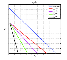
Fig. 8 shows that the rate region for different values of when the is constant. Note that the non-ideal rate region approaches the ideal rate region as decreases, along the axis only. This is because the effects the PU more than the CR. Fig. 9 shows that the rate region for different values of when the is constant. Observe the change in rate region is only on the axis. Fig. 10 gives the rate region when both and vary simultaneously.
IV-A Maximum sum capacity
The sum capacity of CR and PU is given by
| (11) |
The maximum sum rate that the CR and PU can transmit, for a given , can be found out by solving the following optimization problem. The data rate achievable by the CR is
| (12) |
It is easy to verify that the maximum is attained when . The value of sum capacity will then be equal to that in the ideal case.
The inverse problem of the maximum sum rate is when we have a given and and we want to see what value of maximizes the sum capacity.
| (13) |
The objective function can be re-framed as
| (14) |
The solution to this depends upon the term and is given by
| (15) |
V Spectral Efficiency Factor in the Non Ideal Detection
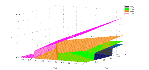
In this section, we use expression of the sum capacity of CR and PU to express spectral efficiency factor in terms of , and . We look for the pairs which result in spectral efficiency factor being more than unity for a given value of corresponding to the case where the sum capacity in the CR system is at least as much as was the capacity of PU alone without CR. Then those pairs are explored which guarantee that the PU’s performance loss is within a limit. All such pairs make up admissible regions. Note that a pair that is not admissible is termed as inadmissible and all such pairs constitute the inadmissible region. Appropriately, we define the two types of regions (i) where the - called weakly admissible region and (ii) where the PU does not loose beyond a limit - called strongly admissible region within a specified loss factor for PU. We also find what pairs that are admissible if the PU cannot incur any loss and term these as strong admissible pairs. We then discuss the effects of , and and show that has more profound effect than on the performance of CR.
The spectral efficiency factor for the non ideal case is as shown below.
Theorem 2.
The spectral efficiency factor in the non ideal case , with average power constraints and for the PU and CR respectively is given by
| (16) |
where and are specified in Lemma 1.
Proof.
In the ideal case the spectral efficiency factor depended only on one parameter , while in the non ideal case here it depends upon and as well. Hence the following corollary helps in studying the rate at which spectral efficiency increases/decreases with change in any one of these parameters keeping the others fixed.
Corollary 2.
Spectral efficiency factor increases with for a fixed with a rate given by
| (17) |
Proof.
By partially differentiating (16) w.r.t we get the result. ∎
Corollary 3.
Spectral efficiency factor decreases with for a fixed with a rate given by
| (18) |
Proof.
By partially differentiating (16) w.r.t we get the result. ∎
Corollary 4.
Spectral efficiency factor decreases with with a rate given by
| (19) |
Proof.
By partially differentiating (16) w.r.t we get the result. ∎
It is interesting to note that the rate of increase in with is independent of . Also the rate of decrease in with is independent of . Moreover, the rate of decrease in with is independent of both and . Hence, we can say that decreases the spectral efficiency factor of the system equally at all occupancies.
Observe from Theorem 2 and Lemma 1 that not all pairs of , will result in the spectral efficiency factor to be greater than one. This is because if there is high then due to interference both CR and PU will have reduced transmission rates. If there is high then the CR will have less transmission rate. To study precisely the effects of and to characterize them in a region for which we define the notion of weak admissibility as follows
Definition 3.
A pair is said to be weakly admissible for a Bernoulli occupancy and average power constraints and on the PU and CR respectively, if the spectral efficiency factor .
When the CR interferes in the PU communication, there will be a loss to the PU. Suppose we are given a limit beyond which the PU cannot incur a loss. It is of interest to see what values of can ensure that the loss to the PU is below this limit. We model this in the form of the loss factor. The loss factor of the PU is the fraction of data rate it looses due to the intervention of the CR in its communication. Formally,
Definition 4.
The loss factor of the PU is
Note that . We now wish to see what will guarantee a loss below . This gives rise to notion of strong admissibility with a loss factor as follows,
Definition 5.
A pair is said to be strongly admissible with a loss factor for a Bernoulli occupancy and average power constraints and on the PU and CR respectively, if . In particular if we say that are strongly admissible.
Now, we characterize the admissible regions based on the above definitions.
V-A Characterization of Admissible Regions
In this subsection we characterize three types of admissible regions viz (i) weakly admissible region - Theorem 3, (ii) strongly admissible region with a loss factor - Theorem 4 and (iii) strongly admissible region - Theorem 5.
Theorem 3.
The pair are weakly admissible if,
-
(1)
.
-
(2)
.
Proof.
The first constraint is kept there to realize that the other constraint can be satisfied for almost all values of if is not confined to the interval of . From definition of weak admissibility
| (20) |
Grouping terms of and together, we have
∎
Observe that the region for strong admissibility with a factor , only depends on . This is because strong admissibility is concerned with the data rate of PU only. For a that is strongly admissible with a factor all values of are admissible. Therefore we plot for strong admissibility. Also we provide characterization of strong admissible regions with a loss factor in terms of only as follows
Theorem 4.
The value of is strongly admissible for a given loss factor of the PU if,
Proof.
Theorem 5.
Strongly admissible region is characterized by .
Proof.
For strong admissibility we have . Thus,
Note that, , hence we have
| (23) |
in the limit would imply that which is never the case. Hence, . ∎
Theorem 5 implies that any detection technique with will lead to spectral efficiency loss for the PU. Since all the practical techniques, will have , we have introduced the notion of strong admissibility with a loss factor.
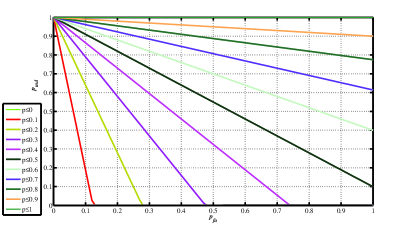
V-B Strong Admissible with a loss factor .
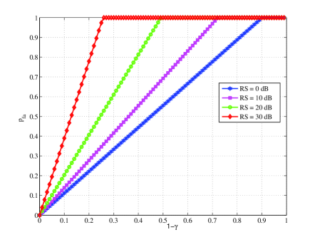
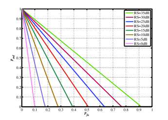
A typical curve of the strongly admissible with a loss factor against is shown in Fig. 12. As we decrease , increases the rate at which the admissible value of increases is .
Theorem 6.
The range of strongly admissible values of for a loss factor is independent of the PU channel occupancy. Furthermore, for a loss factor of the range of values is the entire interval .
Proof.
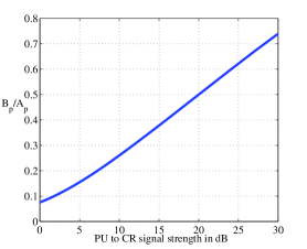
We call as the full admissible point. Observe that for , i.e. the strong admissible case . Also note that the admissible values of are highly dependent on the relative power levels of the PU and CR () transmission. As the value increases the values of strongly admissible for a given loss factor also increases as shown in Fig. 13. Similarly as increases the value of the full admissible point increases as illustrated in Fig. 14.
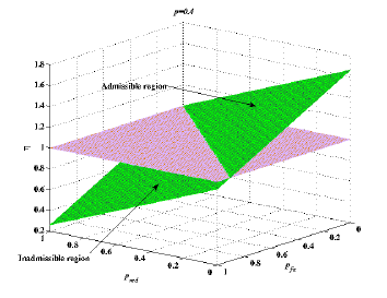
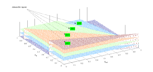
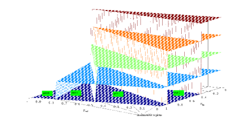
Next we consider the weak admissible region. Fig. 15 shows the spectral efficiency factor plot for a particular value of and with the admissible and inadmissible regions marked. Fig. 16 shows the spectral efficiency factor for various values of for a constant . Observe that the admissible region increase as increases. This implies that for channel with low primary occupancy a lousy detector (with high ) will also result in increase in spectral efficiency. Similarly for the PU will transmit its original capacity without CR and hence any value of would be weakly admissible. Also observe from Fig. 20 that when is fixed and is increased, the admissible region increases. This is justified because, when the is more the CR transmits relatively lesser power which causes lesser interference when compared to when is lower. This translates into higher values of admissible for higher when compared to the lower .
VI Comparison of Various Detection Techniques in light of the Admissible Regions
We compare few of the standard detection techniques viz. energy detection (ed), matched filter (mf) and magnitude squared coherence (msc).
For every detection technique (dt) we have a relation between the and , i.e. for a given average received signal to noise ratio (SNR). The function for all standard detection techniques is monotone non increasing. For a given we wish to see whether any value of is admissible.
Denote . We then wish to find for a detection technique whether for a given , holds. If yes, then we say that the detection technique operating at that pair is admissible and consequently all such points on the curve of detection technique are referred to as admissible region of the detection technique. Note that, this admissible region of a detection technique is dependent on average received SNR.
We provide the functions for three detection techniques mentioned above. In what follows the value of is a function of for all other parameters fixed.
| (24) |
where, is the non central distribution of with degrees of freedom and positive non centrality parameter and is the inverse lower incomplete function. is the standard Q-function with being the inverse function. is as given in [19]. Here, denotes the number of disjoint sequences that an original sequence of length is divided into each of length so that . is the energy of the transmitted signal. is the magnitude squared coherence which is the magnitude squared of the spectral coherence. For more details, the reader is referred to [20] and the references therein.
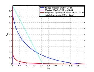
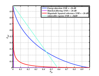
We now plot vs. and look for those areas where the curve of detection region lies inside the weak admissible region. For all points lying on that part of the curve the detection technique is admissible.
Figs. 21, 22 show that, for low SNR regimes, all values of offered by the matched filter detector are admissible. For the magnitude squared coherence detector majority of the points on the curve are admissible except those at higher end of values. For the energy detector many points on the curve lie outside the admissible region. Hence, using energy detector, one has to be careful about the operating point . It follows that the matched filter performs better than magnitude squared coherence detector which performs better than the energy detector. These observations are in line with those in [21].
VII Conclusion
In this paper we have capacity region of a point to point CR channel. For ideal detection of PU occupancy we have seen the limits on rates. We have defined spectral efficiency factor and studied its variations with respect to the occupancy probability for different relative power levels of the PU and CR. Then we built the case where the CR performs non ideal detection of the PU presence and specified capacity region for the same. With expressions derived we brought out the limits, under different occupancies and relative PU and CR power levels, on the false alarm and missed detection for which the spectral efficiency of the overall system increases and also for which the PU is not at a loss greater than a specified value. We have discussed the effects of false alarm, missed detection and channel occupancy with respect to spectral efficiency factor. Finally we compared our result with standard detection techniques viz. energy detection, matched filter and magnitude squared coherence and found that the matched filter performs best followed by magnitude squared coherence followed by energy detection with respect to spectral efficiency factor.
Acknowledgment
The work was sponsored by Department of Information Technology, Government of India, under the grant for the project “High Performance Cognitive Radio Networks at IIT Bombay and IIT Hyderabad”.
References
- [1] FCC, “Report of the spectrum efficiency working group,” FCC Spectrum policy task force Tech Rep, 2002.
- [2] I. Mitola, J. and J. Maguire, G.Q., “Cognitive radio: making software radios more personal,” Personal Communications, IEEE, vol. 6, pp. 13 –18, aug 1999.
- [3] A. M. Wyglinski, M. Nekovee, and Y. T. Hou, Cognitive Radio Communications and Networks: Principles and Practice. Academic Press, 2009.
- [4] A. Goldsmith, S. Jafar, I. Maric, and S. Srinivasa, “Breaking spectrum gridlock with cognitive radios: An information theoretic perspective,” Proceedings of the IEEE, vol. 97, pp. 894 –914, may 2009.
- [5] S. Srinivasa and S. Jafar, “The throughput potential of cognitive radio: A theoretical perspective,” in Signals, Systems and Computers, 2006. ACSSC ’06. Fortieth Asilomar Conference on, pp. 221 –225, 29 2006-nov. 1 2006.
- [6] N. Devroye, P. Mitran, and V. Tarokh, “Achievable rates in cognitive radio channels,” Information Theory, IEEE Transactions on, vol. 52, pp. 1813 – 1827, may 2006.
- [7] W. Wu, S. Vishwanath, and A. Arapostathis, “Capacity of a class of cognitive radio channels: Interference channels with degraded message sets,” Information Theory, IEEE Transactions on, vol. 53, pp. 4391 –4399, nov. 2007.
- [8] A. Jovicic and P. Viswanath, “Cognitive radio: An information-theoretic perspective,” Information Theory, IEEE Transactions on, vol. 55, pp. 3945 –3958, sept. 2009.
- [9] K. G. Nagananda, P. Mohapatra, C. R. Murthy, and S. Kishore, “Multiuser cognitive radio networks: An information theoretic perspective,” CoRR, vol. abs/1102.4126, 2011.
- [10] L. Musavian and S. Aïssa, “Fundamental capacity limits of cognitive radio in fading environments with imperfect channel information,” Trans. Comm., vol. 57, pp. 3472–3480, Nov. 2009.
- [11] N. Yi, Y. Ma, and R. Tafazolli, “Underlay cognitive radio with full or partial channel quality information,” CoRR, vol. abs/1009.2927, 2010.
- [12] K. Son, B. C. Jung, S. Chong, and D. K. Sung, “Opportunistic underlay transmission in multi-carrier cognitive radio systems,” in Proceedings of the 2009 IEEE conference on Wireless Communications & Networking Conference, WCNC’09, (Piscataway, NJ, USA), pp. 1365–1370, IEEE Press, 2009.
- [13] G. Bansal, O. Duval, and F. Gagnon, “Joint overlay and underlay power allocation scheme for ofdm-based cognitive radio systems,” in Vehicular Technology Conference (VTC 2010-Spring), 2010 IEEE 71st, pp. 1 –5, may 2010.
- [14] L. Li and M. Pesavento, “The sum capacity of underlay cognitive broadcast channel,” in Cognitive Radio Oriented Wireless Networks and Communications (CROWNCOM), 2011 Sixth International ICST Conference on, pp. 390 –394, june 2011.
- [15] R. Zhang, S. Cui, and Y.-C. Liang, “On ergodic sum capacity of fading cognitive multiple-access and broadcast channels,” IEEE Trans. Inf. Theor., vol. 55, pp. 5161–5178, Nov. 2009.
- [16] A. Gibson and L. Arnett, “Statistical modelling of spectrum occupancy,” Electronics Letters, vol. 29, pp. 2175 –2176, dec. 1993.
- [17] S. M. Kay, Fundamentals of Statistical Signal Processing, Volume 2: Detection Theory. Prentice Hall PTR, Jan. 1998.
- [18] D. Tse and P. Viswanath, Fundamentals of wireless communication. New York, NY, USA: Cambridge University Press, 2005.
- [19] G. Carter, C. Knapp, and A. Nuttall, “Estimation of the magnitude-squared coherence function via overlapped fast fourier transform processing,” Audio and Electroacoustics, IEEE Transactions on, vol. 21, pp. 337 – 344, aug 1973.
- [20] D. Bhargavi and C. Murthy, “Performance comparison of energy, matched-filter and cyclostationarity-based spectrum sensing,” in Signal Processing Advances in Wireless Communications (SPAWC), 2010 IEEE Eleventh International Workshop on, pp. 1 –5, june 2010.
- [21] B. Wang and K. Liu, “Advances in cognitive radio networks: A survey,” Selected Topics in Signal Processing, IEEE Journal of, vol. 5, pp. 5 –23, feb. 2011.