Relation between baryon number fluctuations and experimentally observed proton number fluctuations in relativistic heavy ion collisions

Abstract

We explore the relation between proton and nucleon number fluctuations in the final state in relativistic heavy ion collisions. It is shown that the correlations between the isospins of nucleons in the final state are almost negligible over a wide range of collision energy. This leads to a factorization of the distribution function of the proton, neutron, and their antiparticles in the final state with binomial distribution functions. Using the factorization, we derive formulas to determine nucleon number cumulants, which are not direct experimental observables, from proton number fluctuations, which are experimentally observable in event-by-event analyses. With a simple treatment for strange baryons, the nucleon number cumulants are further promoted to the baryon number ones. Experimental determination of the baryon number cumulants makes it possible to compare various theoretical studies on them directly with experiments. Effects of nonzero isospin density on this formula are addressed quantitatively. It is shown that the effects are well suppressed over a wide energy range.

I Introduction

Now that the observation of the quark-gluon matter in relativistic heavy ion collisions is established for small baryon chemical potential ($\mu_{\rm B}$) RHIC , a challenging experimental subject following this achievement is to reveal the global structure of the QCD phase diagram on the temperature ($T$) and $\mu_{\rm B}$ plane. In particular, finding the QCD critical point(s), whose existence is predicted by various theoretical studies Asakawa:1989bq ; Stephanov:2004wx , is one of the most intriguing problems. Since the $\mu_{\rm B}$ of the hot medium created by heavy-ion collisions can be controlled by varying the collision energy per nucleon pair, $\sqrt{s_{\rm NN}}$, the $\mu_{\rm B}$ dependence of the nature of QCD phase transition should be observed as the $\sqrt{s_{\rm NN}}$ dependence of observables. An experimental project to explore such signals in the energy range $10{\rm GeV}\lesssim\sqrt{s_{\rm NN}}\lesssim 200{\rm GeV}$, which is called the energy scan program, is now ongoing at the Relativistic Heavy Ion Collider (RHIC) Aggarwal:2010wy ; Mohanty:2011nm . Experimental data which will be obtained in future experimental facilities designed for lower beam-energy collisions will also provide important information on this subject Bleicher:2011jk .

Observables which are suitable to analyze bulk properties of the matter around the phase boundary of QCD in heavy ion collisions are fluctuations Koch:2008ia . Experimentally, fluctuations are measured through event-by-event analyses Aggarwal:2010wy . Theoretically, it is predicted that some of them, including higher-order cumulants, are sensitive to critical behavior near the QCD critical point Stephanov:1998dy ; Hatta:2003wn ; Stephanov:2008qz ; Athanasiou:2010kw ; Fraga:2011hi , and/or locations on the phase diagram, especially on which side the system is, the hadronic side or the quark-gluon side Asakawa:2000wh ; Jeon:2000wg ; Koch:2005vg ; Ejiri:2005wq ; Asakawa:2009aj ; Friman:2011pf ; Stephanov:2011pb .

Among the fluctuation observables, those of conserved charges are believed to possess desirable properties to probe the phase structure in relativistic heavy ion collisions. One of the advantages of using the conserved charges is that the characteristic times for the variation of their local densities are longer than those for non-conserved ones, because the variation of the local densities of conserved charges are achieved only through diffusion Asakawa:2000wh ; Jeon:2000wg . The fluctuations of the former thus can better reflect fluctuations generated in earlier stages of fireballs, when the rapidity coverage is taken sufficiently large. From a theoretical point of view, an important property of the conserved charges is that one can define the operator of a conserved charge, $Q$, as a Noether current. Moreover, their higher-order cumulants, $\langle\delta Q^{n}\rangle_{c}$, are directly related to the grand canonical partition function $Z(\mu)={\rm Tr}e^{-\beta(H-\mu Q)}$ as

$$\langle\delta Q^{n}\rangle_{c}=T^{n}\frac{\partial^{n}\log Z(\mu)}{\partial\mu^{n}},$$ (1)

with $H$ and $\mu$ being the hamiltonian and the chemical potential associated with $Q$, respectively. These properties make the analysis of cumulants of conserved charges well defined and feasible in a given theoretical framework. For example, they can be measured in lattice QCD Monte Carlo simulations Gavai:2010zn ; Schmidt:2010xm ; Mukherjee:2011td ; Borsanyi:2011sw ; Bazavov:2012jq . The relation Eq. (1) also provides an intuitive interpretation for the behavior of higher-order cumulants of conserved charges. For instance, the third-order cumulant of the net baryon number, $N_{\rm B}^{\rm(net)}$, satisfies $\langle(\delta N_{\rm B}^{\rm(net)})^{3}\rangle_{c}=T\partial\langle(\delta N_{\rm B}^{\rm(net)})^{2}\rangle_{c}/\partial\mu_{\rm B}$. This formula means that $\langle(\delta N_{\rm B}^{\rm(net)})^{3}\rangle_{c}$ changes its sign around the phase boundary on the $T$-$\mu_{\rm B}$ plane where the baryon number susceptibility $\langle(\delta N_{\rm B}^{\rm(net)})^{2}\rangle$ has a peak structure Asakawa:2009aj . The change of the sign of observables like this will serve as a clear experimental signal Asakawa:2009aj ; Friman:2011pf ; Stephanov:2011pb .

QCD has several conserved charges, such as baryon and electric charge numbers and energy. Among these conserved charges, theoretical studies suggest that the cumulants of the baryon number have the most sensitive dependences on the phase transitions and phases of QCD. In order to see this feature, let us compare the baryon number cumulants with the electric charge ones. First, the baryon number fluctuations show the critical fluctuations associated with the QCD critical point more clearly. Although the baryon and electric charge number fluctuations diverge with the same critical exponent around the critical point, it should be remembered that this does not mean similar clarity of signals for the critical enhancement in experimental studies. Fluctuations near the critical point are generally separated into singular and regular parts, and only the former diverges with the critical exponent. The singular part of the electric charge fluctuations is relatively suppressed compared to the baryon number ones, because the formers contain the isospin number fluctuations which are regular near the critical point Hatta:2003wn . The additional regular contribution makes the experimental confirmation of the enhancement of the singular part difficult, and this tendency is more pronounced in higher-order cumulants Asakawa:2009aj . While it is known that the proton number fluctuations in the final state also reflect the critical enhancement near the critical point Hatta:2003wn , as we will show later the baryon number fluctuations are superior to this observable, too, in the same sense. Second, the ratios of baryon number cumulants Ejiri:2005wq behave more sensitively to the difference of phases, i.e., hadrons, or quarks and gluons. This is because the ratios are dependent on the magnitude of charges carried by the quasi-particles composing the state Asakawa:2000wh ; Jeon:2000wg ; Ejiri:2005wq , while the charge difference between hadrons and quarks is more prominent in the baryon number.

Experimentally, however, the baryon number fluctuations are not directly observable, because chargeless baryons, such as neutrons, cannot be detected by most detectors. Proton number fluctuations can be measured Aggarwal:2010wy ; Mohanty:2011nm , and recently its cumulants have been compared with theoretical predictions for baryon number cumulants. Indeed, in the free hadron gas in equilibrium the baryon number cumulants are approximately twice the proton number ones, because the baryon number cumulants in free gas are simply given by the sum of those for all baryons, and the baryon number is dominated by proton and neutron numbers in the hadronic medium relevant to relativistic heavy ion collisions. In general, however, these cumulants behave differently. In fact, we will see later that the non-thermal effects which exists in baryon number cumulants are strongly suppressed in the proton number ones.

In heavy ion collisions, because of the dynamical evolution the medium at kinetic freezeout is not completely in the thermal equilibrium. The original ideas to exploit fluctuation observables as probes of primordial properties of fireballs Asakawa:2000wh ; Jeon:2000wg are concerned with this non-thermal effect encoded in the final state as a hysteresis of the time evolution. To observe such effects, it is highly desirable to measure baryon number cumulants that is expected to retain more effects of the phase transition and the singularity around the critical point. The experimental determination of baryon number cumulants also makes the comparison between experimental and theoretical studies more robust, since many theoretical works including lattice QCD simulations are concerned with the baryon number cumulants, not the proton number ones.

In Ref. Kitazawa:2011wh , the authors of the present paper have argued that, whereas the baryon number cumulants are not the direct experimental observables as discussed above, they can be determined in experiments by only using the experimentally measured proton number fluctuations for $\sqrt{s_{\rm NN}}\gtrsim 10{\rm GeV}$. The key idea is that isospins of nucleons in the final state are almost completely randomized and uncorrelated, because of reactions of nucleons with thermal pions in the hadronic stage, as will be elucidated in Sec. II. This leads to the conclusion that, when $N_{\rm N}$ nucleons exist in a phase space of the final state, the probability that $N_{p}$ nucleons among them are protons follows the binomial distribution. More generally, the probability distribution that $N_{p}$ protons, $N_{n}$ neutrons, $N_{\bar{p}}$ anti-protons, and $N_{\bar{n}}$ anti-neutrons are found in the final state in a phase space is factorized as

$${\cal P}_{\rm N}(N_{p},N_{n},N_{\bar{p}},N_{\bar{n}})$$

$$={\cal F}(N_{\rm N},N_{\bar{\rm N}})B_{r}(N_{p};N_{\rm N})B_{\bar{r}}(N_{\bar{p}};N_{\bar{\rm N}}),$$ (2)

where the nucleon and anti-nucleon numbers are $N_{\rm N}=N_{p}+N_{n}$ and $N_{\bar{\rm N}}=N_{\bar{p}}+N_{\bar{n}}$, respectively, and

$$B_{r}(k;n)=\frac{n!}{k!(n-k)!}r^{k}(1-r)^{n-k}$$ (3)

is the binomial distribution function with probabilities $r=\langle N_{p}\rangle/\langle N_{\rm N}\rangle$ and $\bar{r}=\langle N_{\bar{p}}\rangle/\langle N_{\bar{\rm N}}\rangle$. The function ${\cal F}(N_{\rm N},N_{\bar{\rm N}})$ describes the distribution of nucleons and anti-nucleons and the correlation between them in the final state, which are determined by the dynamical history of fireballs. Using the factorization Eq. (2), one can obtain formulas to represent the (anti-)nucleon number cumulants by the (anti-)proton number ones, and vice versa; whereas the neutron number is not determined by experiments, this missing information can be reconstructed with the knowledge for the distribution function, Eq. (2). The (anti-)nucleon number in Eq. (2) can further be promoted to the (anti-)baryon number in practical analyses with a simple treatment for strange baryons to a good approximation. These formulas enable to determine the baryon number cumulants solely with the experimentally measured proton number fluctuations, and, as a result, to obtain insights into the present experimental results on the proton number cumulants.

The main purpose of the present paper is to elaborate the discussion in Ref. Kitazawa:2011wh with some extensions. In Ref. Kitazawa:2011wh the formulas are derived only for isospin symmetric medium. In the present study we extend them to incorporate cases with nonzero isospin densities. With the extended relations, it is shown that the effect of nonzero isospin density is well suppressed for $\sqrt{s_{\rm NN}}\gtrsim 10{\rm GeV}$. The procedures of the manipulations and discussions omitted in Ref. Kitazawa:2011wh are also addressed in detail.

In the next Section, we show that the factorization Eq. (2) is well applied to the nucleon and baryon distribution functions in the final state in heavy ion collisions. We then derive formulas to relate baryon and proton number cumulants in Sec. III. In Sec. IV, we discuss the recent experimental results at STAR Aggarwal:2010wy ; Mohanty:2011nm using the results in Sec. III, and possible extensions of our results. The final section is devoted to a short summary.

Throughout this paper, we use $N_{X}$ to represent the number of particles $X$ leaving the system after each collision event, where $X=p$, $n$, N, and B represent proton, neutron, nucleon, and baryon, respectively, and their anti-particles, $\bar{p}$, $\bar{n}$, $\bar{\rm N}$, and $\bar{\rm B}$. The net and total numbers are defined as $N_{X}^{\rm(net)}=N_{X}-N_{\bar{X}}$ and $N_{X}^{\rm(tot)}=N_{X}+N_{\bar{X}}$, respectively.

II Distribution function for proton and neutron numbers

In this section, we discuss the time evolution of the proton and neutron number distributions in the hadronic medium generated by relativistic heavy ion collisions, and show that the nucleon distribution in the final state in a phase space is factorized as in Eq. (2) at sufficiently large $\sqrt{s_{\rm NN}}$. In Sec. II.1, as a preliminary example we show that Eq. (2) is applicable to the equilibrated free hadron gas in the ranges of $T$ and $\mu_{\rm B}$ relevant to relativistic heavy ion collisions. We then extend the argument to the distribution function in the final state in relativistic heavy ion collisions in Sec. II.2.

II.1 Free hadron gas in equilibrium

Let us first consider nucleons in the free hadron gas in equilibrium. For $T$ and $\mu_{\rm B}$ which are relevant to relativistic heavy ion collisions, the nucleon mass $m_{\rm N}$ satisfies $m_{\rm N}-|\mu_{\rm B}|\gg T$. One thus can apply the Boltzmann approximation for the distribution functions of nucleons. The number of particles in a phase space, $N$, which obey Boltzmann statistics is given by the Poisson distribution,

$$P_{\lambda}(N)=\frac{e^{-\lambda}\lambda^{N}}{N!},$$ (4)

with the average $\lambda=\langle N\rangle=\sum_{N}NP_{\lambda}(N)$. Accordingly, the probability to find $N_{p}$ ($N_{\bar{p}}$) protons (anti-protons) and $N_{n}$ ($N_{\bar{n}}$) neutrons (anti-neutrons) in the phase space is given by the product of the Poisson distribution functions,

$${\cal P}_{\rm HG}(N_{p},N_{n},N_{\bar{p}},N_{\bar{n}})$$

$$=P_{\langle N_{p}\rangle}(N_{p})P_{\langle N_{n}\rangle}(N_{n})P_{\langle N_{\bar{p}}\rangle}(N_{\bar{p}})P_{\langle N_{\bar{n}}\rangle}(N_{\bar{n}}).$$ (5)

The product of two Poisson distribution functions satisfies the identity,

$$P_{\lambda_{1}}(N_{1})P_{\lambda_{2}}(N_{2})$$

$$=P_{\lambda_{1}+\lambda_{2}}(N_{1}+N_{2})B_{\lambda_{1}/(\lambda_{1}+\lambda_{2})}(N_{1};N_{1}+N_{2}),$$ (6)

where $B_{r}(k;n)$ is the binomial distribution function Eq. (3). Using Eq. (6), Eq. (5) is rewritten as

$${\cal P}_{\rm HG}(N_{p},N_{n},N_{\bar{p}},N_{\bar{n}})$$

$$=P_{\langle N_{\rm N}\rangle}(N_{\rm N})P_{\langle N_{\bar{\rm N}}\rangle}(N_{\bar{\rm N}})B_{r}(N_{p};N_{\rm N})B_{\bar{r}}(N_{\bar{p}};N_{\bar{\rm N}}),$$ (7)

where $N_{\rm N}=N_{p}+N_{n}$ and $N_{\bar{\rm N}}=N_{\bar{p}}+N_{\bar{n}}$ are the nucleon and anti-nucleon numbers, respectively, and $r=\langle N_{p}\rangle/\langle N_{\rm N}\rangle$ and $\bar{r}=\langle N_{\bar{p}}\rangle/\langle N_{\bar{\rm N}}\rangle$. Equation (7) shows that the distribution of nucleons in the free hadron gas is factorized using binomial functions as in Eq. (2) with

$${\cal F}(N_{\rm N},N_{\bar{\rm N}})=P_{\langle N_{\rm N}\rangle}(N_{\rm N})P_{\langle N_{\bar{\rm N}}\rangle}(N_{\bar{\rm N}}).$$ (8)

The appearance of the binomial distribution functions in Eq. (7) is understood as follows. When one finds a nucleon in the hadron gas, the probability that the nucleon is a proton is $r$. The isospins of all nucleons found in the phase space, moreover, are not correlated with one another as a consequence of Boltzmann statistics and the absence of interactions. Once $N_{\rm N}$ nucleons are found in the phase space, therefore, the probability that $N_{p}$ particles are protons is a superposition of independent events with probability $r$, i.e., the binomial distribution.

We note that the above discussion is not applicable when the condition $m_{\rm N}-|\mu_{\rm B}|\gg T$, required for Boltzmann statistics, is not satisfied. When quantum correlations of nucleons arising from Fermi statistics are not negligible, the isospin of each nucleon can no longer be independent. As long as we are concerned with the range of $T$ and $\mu_{\rm B}$ which can be realized by relativistic heavy ion collisions, however, the condition for the Boltzmann approximation is well satisfied except in very low energy collisions Cleymans:1998fq .

II.2 Final state in heavy ion collisions

Next, we consider the nucleon distribution functions in the final state in heavy ion collisions. We show that the nucleon distribution in this case is also factorized as in Eq. (2), by demonstrating that the isospins of all nucleons in the final state are random and uncorrelated.

II.2.1 $\Delta(1232)$ resonance

The key ingredient to obtain the factorization Eq. (2) in the final state in relativistic heavy ion collisions is ${\rm N}\pi$ reactions in the hadronic stage mediated by $\Delta(1232)$ resonances having the isospin $I=3/2$. As we will see later, this is the most dominant reaction of nucleons in the hadronic medium. This is because i) the cross section of ${\rm N}\pi\to\Delta$ reactions exceeds $200{\rm mb}=20{\rm fm}^{2}$ and is comparable with ${\rm NN}$ and ${\rm N\bar{N}}$ reactions for $P_{\rm lab}\simeq 300{\rm MeV}$ PDG , and ii) the pion density dominates over those of all other particles in the ranges of $T$ and $\mu_{\rm B}$ accessible with heavy ion collisions at $\sqrt{s_{\rm NN}}\gtrsim 10{\rm GeV}$; at the top RHIC energy, the density of pions is more than one order larger than that of nucleons. We shall show below that these reactions frequently take place even after chemical freezeout in the hadronic medium during the time evolution of the fireballs.

The ${\rm N}\pi$ reactions through $\Delta$ contain charge exchange reactions, which alter the isospin of the nucleon in the reaction. The reactions of a proton to form $\Delta$ are:

$$p+\pi^{+} \to\Delta^{++}\to p+\pi^{+},$$ (9)

$$p+\pi^{0} \to\Delta^{+}\to p(n)+\pi^{0}(\pi^{+}),$$ (10)

$$p+\pi^{-} \to\Delta^{0}\to p(n)+\pi^{-}(\pi^{0}).$$ (11)

Among these reactions, Eqs. (10) and (11) are responsible for the change of the nucleon isospin. The ratio of the cross sections of a proton to form $\Delta^{++}$, $\Delta^{+}$, and $\Delta^{0}$ is $3:1:2$, which is determined by the isospin SU(2) symmetry of the strong interaction. The isospin symmetry also tells us that the branching ratios of $\Delta^{+}$ ($\Delta^{0}$) decaying into the final state having a proton and a neutron are $1:2$ ($2:1$). Using these ratios, one obtains the ratio of the probabilities that a proton in the hadron gas forms $\Delta^{+}$ or $\Delta^{0}$ with a reaction with a thermal pion, and then decays into a proton and a neutron, respectively, $P_{p\to p}$ and $P_{p\to n}$, as

$$P_{p\to p}:P_{p\to n}=5:4,$$ (12)

provided that the hadronic medium is isospin symmetric and that the three isospin states of the pion are equally distributed in the medium. Because of the isospin symmetry of the strong interaction one also obtains the same conclusion for neutron reactions:

$$P_{n\to n}:P_{n\to p}=5:4.$$ (13)

Similar results are also obtained for anti-nucleons. Equations (12) and (13) show that these reactions act to randomize the isospin of nucleons during the hadronic stage.

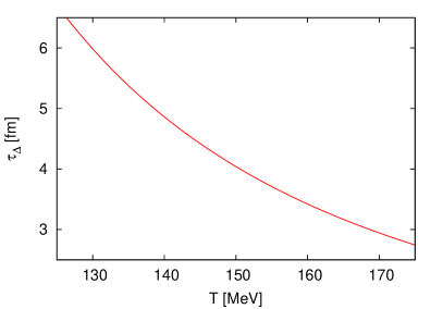
Figure 1: Mean time $\tau_{\Delta}$ of a rest nucleon to form $\Delta^{+}$ or $\Delta^{0}$ in the hadronic medium as a function of temperature $T$.

II.2.2 Mean time

Next, let us estimate the mean time of these reactions. Assuming that pions are thermally distributed, the mean time $\tau_{\Delta}$ of a nucleon at rest in the medium to undergo a reaction Eq. (10) or (11) is given by

$$\tau_{\Delta}^{-1}=\int\frac{d^{3}k_{\pi}}{(2\pi)^{3}}\sigma(E_{\rm c.m.})v_{\pi}n(E_{\pi}),$$ (14)

with the Bose distribution function $n(E)=(e^{E/T}-1)^{-1}$, the pion momentum $k_{\pi}$, the pion velocity $v_{\pi}=k_{\pi}/E_{\pi}$, $E_{\pi}=\sqrt{m_{\pi}^{2}+k_{\pi}^{2}}$, and the pion mass $m_{\pi}$. $\sigma(E_{\rm c.m.})$ is the sum of the cross sections for N$\pi$ reactions producing $\Delta^{+}$ and $\Delta^{0}$ for the center-of-mass energy $E_{\rm c.m.}=[(m_{\rm N}+E_{\pi})^{2}-k_{\pi}^{2}]^{1/2}$ with the nucleon mass $m_{\rm N}$. For the cross section $\sigma(E_{\rm c.m.})$, we assume that the peak corresponding to $\Delta(1232)$ resonance is well reproduced by the Breit-Wigner form,

$$\sigma(E_{\rm c.m.})=\sigma_{\Delta}\frac{\Gamma^{2}/4}{(E_{\rm c.m.}-m_{\Delta})^{2}+\Gamma^{2}/4},$$ (15)

which is a sufficient approximation for our purpose. Here, we use the value of the parameters determined by the N$\pi$ reactions in the vacuum, $m_{\Delta}=1232{\rm MeV}$, $\Gamma=110{\rm MeV}$, and $\sigma_{\Delta}=20{\rm fm}^{2}$ PDG . The medium effects on the cross section will be discussed later. Substituting $m_{\rm N}=940{\rm MeV}$ and $m_{\pi}=140{\rm MeV}$, one obtains the $T$ dependence of the mean time $\tau_{\Delta}$ presented in Fig. 1. The figure shows that the mean time is $\tau_{\Delta}=3\sim 4$fm for $T=150\sim 170{\rm MeV}$. One can confirm that the mean time hardly changes even for moving nucleons in the range of momentum $p\lesssim 3T$ by extending Eq. (14) to cases with nonzero nucleon momentum. The lifetime of $\Delta$ resonances is $\tau_{\Gamma}=1/\Gamma\simeq 1.8{\rm fm}$.

The mean time evaluated above is much shorter than the lifetime of the hadronic stage in relativistic heavy ion collisions. According to a dynamical model analysis for collisions at RHIC, nucleons in the hadron phase continue to interact for a couple of tens of fm on average at midrapidity Nonaka:2006yn . As a result, at the RHIC energy each nucleon in a fireball has chances to undergo the charge exchange reactions several times in the hadronic stage.

Two remarks are in order here. First, the above result on the time scales shows that the reactions to produce $\Delta$ proceed even after chemical freezeout. These reactions do not contradict the success of the statistical model, which describes the chemical freezeout BraunMunzinger:2003zd , because chemical freezeout is a concept to describe ratios of particle abundances such as $\langle N_{\bar{p}}\rangle/\langle N_{p}\rangle$ and the above reactions do not alter the average abundances in the final state. The success of the model, on the other hand, indicates that creations and annihilations of (anti-)nucleons hardly occur after chemical freezeout. Second, we note that the dynamical model in Ref. Nonaka:2006yn uses an equation of states having a first order phase transition in the hydrodynamic simulations for the time evolution above the critical temperature $T_{\rm c}$. Recently, dynamical simulations have been carried out with more realistic equations of states obtained by lattice QCD simulations Schenke:2010nt . The lifetime of hadronic stage evaluated in these studies is more relevant to this argument. We, however, note that the qualitative behavior of the time evolution seems not sensitive to the difference in equations of states Schenke:2010nt .

While N$\pi$ reactions frequently take place even below the chemical freezeout temperature, $T_{\rm chem}$, ${\rm N}\bar{\rm N}$ annihilatios and productions almost terminate at $T_{\rm chem}$. This is necessary for the success of the thermal model. For $E_{\rm c.m.}\simeq T$ the cross section of the ${\rm N}\bar{\rm N}$ pair annihilation is largest among all NN and N$\bar{\rm N}$ reactions. If nucleons and anti-nucleons are distributed without correlation, therefore, all NN and N$\bar{\rm N}$ reactions cease to take place at $T_{\rm chem}$. This conclusion is, of course, obtained also by evaluating the mean time for each reaction using the cross sections PDG as in Eq. (14). After chemical freezeout, the only inelastic reactions nucleons go through are thus Eqs. (10) and (11), and after each reaction the nucleon loses its initial isospin information. Only after repeating the reactions Eq. (12) twice, the ratio becomes $41:40$, which is almost even. If medium effects on the formations and decays of $\Delta$ are negligible, therefore, irrespective of the nucleon distribution at the chemical freezeout, the isospin of nucleons at the kinetic freezeout can be regarded random and uncorrelated. On the other hand, the nucleon number distribution can have a deviation from the Boltzmann distribution reflecting the dynamical history of fireballs.

Because of the absence of correlations between isospins of nucleons in the final state, once $N_{\rm N}$ ($N_{\bar{\rm N}}$) nucleons (anti-nucleons) exist in a phase space in the final state, their isospin distribution is simply given by the binomial one. This conclusion leads to the factorization Eq. (2) for proton and neutron number distribution in the final state for an arbitrary phase space. In particular, the final state proton and anti-proton number distribution is written as

$${\cal G}(N_{p},N_{\bar{p}}) =\sum_{N_{n},N_{\bar{n}}}{\cal P}_{\rm N}(N_{p},N_{n},N_{\bar{p}},N_{\bar{n}})$$

$$=\sum_{N_{\rm N},N_{\bar{\rm N}}}{\cal F}(N_{\rm N},N_{\bar{\rm N}})B_{r}(N_{p};N_{\rm N})B_{\bar{r}}(N_{\bar{p}};N_{\bar{\rm N}}).$$ (16)

Unlike in the simple example in Sec. II.1, the nucleon distribution function ${\cal F}(N_{\rm N},N_{\bar{\rm N}})$ in this case is determined by the time evolution of fireballs and is not necessary of a thermal or separable form as in Eq. (8); no specific form for ${\cal F}(N_{\rm N},N_{\bar{\rm N}})$ is assumed here or will be assumed in the analyses in Sec. III. What we have used here is the fact that the time scale for the exchange of isospins between nucleons and pions is sufficiently short compared to the lifetime of hadronic stage after the chemical freezeout. On the other hand, the time scale for the variation of a conserved charge in a phase space depends on the form of the phase space, and can become arbitrary long by increasing the spatial volume. When the time scale is long, the information of the physics of the early stages is encoded in ${\cal F}(N_{\rm N},N_{\bar{\rm N}})$.

II.2.3 Medium effects

Next, let us inspect the possibility of medium effects on the formation and decay rates of $\Delta$. In medium, the decay rate of $\Delta$ acquires the statistical factor,

$$\left(1-f(E_{\rm N})\right)\left(1+n(E_{\pi})\right),$$ (17)

where $f(E)=(e^{(E-\mu_{\rm B})/T}+1)^{-1}$ is the Fermi distribution function and $E_{\rm N}$ and $E_{\pi}$ are the energies of the nucleon and pion produced by the decay, respectively. The first term in Eq. (17) represents the Pauli blocking effect. At the RHIC energy, since the Boltzmann approximation is well applied to nucleons, the Pauli blocking effect is suppressed. The Bose factor $(1+n(E_{\pi}))$ in Eq. (17), on the other hand, has a non-negligible contribution since $m_{\pi}\simeq T_{\rm chem}$. As long as all $n(E_{\pi})$ for the three isospin states of the pion are the same, however, this factor does not alter the branching ratios Eqs. (12) and (13), while the factor enhances the decay of $\Delta$. A possible origin for the variation of $n(E_{\pi})$ is the isospin density of nucleon number; since the isospin density is locally conserved, the isospin density of pions is affected by the nucleon isospin. This effect on $n(E_{\pi})$ is, however, well suppressed since the density of pions is much larger than that of nucleons below $T_{\rm chem}$. Another possible source which gives rise to a different pion distribution is the event-by-event fluctuation of the isospin density in the phase space at the hadronization. It is, however, expected that the effect is well suppressed, again because of the large pion density. One, therefore, can conclude that the medium effect hardly changes the branching ratios Eqs. (12) and (13). The same conclusion also applies to the formation rate of $\Delta$, since the medium effect on the probabilities of a nucleon to undergo reactions Eqs. (9) - (11) depends only on $n(E_{\pi})$. After all, all medium effects on the ratios Eqs. (12) and (13) are negligible.

When the system has a nonzero isospin density, probabilities Eqs. (12) and (13) receive modifications because the three isospin states of the pion are not equally distributed, although this effect is not large as will be shown in Sec. III.4. Even in this case, however, the only modification to the above conclusion is to replace the probabilities $r$ and $\bar{r}$ with appropriate values, since the reactions Eqs. (9) - (11) still act to randomize the nucleon isospins with the modified probabilities determined by the detailed balance condition.

Here, we emphasize that the large pion density in the hadronic medium is responsible for the validity of Eq. (16) in the final state. In the hadronic medium, there are so many pions which can be regarded as a heat bath when the nucleon sector is concerned, while nucleons are so dilutely distributed that they do not feel other ones’ existence.

So far, we have limited our attention to reactions mediated by $\Delta(1232)$. Interactions of nucleons with other mesons, however, can also take place in the hadronic medium, while they are much less dominant. It is also possible that $\Delta$ interacts with thermal pions to form another resonance before its decay Pang:1992sk . All these reactions with thermal particles, however, proceed with certain probabilities determined by the isospin SU(2) symmetry as long as they are caused by the strong interaction. Each reaction of a nucleon thus makes its isospin random, and act to realize the factorization Eq. (2).

II.2.4 Low beam-energy region

The factorization Eq. (16) is fully established for the RHIC energy. At very low beam energy, however, pions are not produced enough and the duration of the hadron phase below $T_{\rm chem}$ becomes shorter. Nucleons, therefore, will not undergo sufficient charge exchange reactions below $T_{\rm chem}$. When the reactions hardly occur, the isospin correlations generated at the hadronization remain until the final state. At low beam energy, also the density of the nucleon becomes comparable to that of pions, and pions can no longer be regarded as a heat bath to absorb isospin fluctuations of nucleons. The requirements to justify the factorization Eq. (16), therefore, eventually breaks down as the beam energy is decreased. This would happen when $T_{\rm chem}\lesssim m_{\pi}$, since the abundance of pions is responsible for all of the above conditions. From the $\sqrt{s_{\rm NN}}$ dependence of the chemical freezeout line on the $T$-$\mu_{\rm B}$ plane Cleymans:1998fq , the factorization Eq. (16) should be well-satisfied in the range of beam energy $\sqrt{s_{\rm NN}}\gtrsim 10$GeV.

II.3 Strange baryons

So far, we have limited our attention to nucleons. Since baryons in the final state in heavy ion collisions are dominated by nucleons, the nucleon number, which is not a conserved charge, is qualitatively identified with the baryon one. It is, however, important to recognize the difference between these two fluctuation observables especially in considering higher-order cumulants. The difference predominantly comes from strange baryons $\Lambda$ and $\Sigma$. In this subsection, we argue a practical method to include the effect of these degrees of freedom in our factorization formula.

Strange baryons produced in the hadronic medium decay via the weak or electromagnetic interaction outside the fireball. $\Lambda$ decays via the weak interaction into $p\pi^{-}$ and $n\pi^{0}$ with the branching ratio

$$P_{\Lambda\to p}:P_{\Lambda\to n}\simeq 16:9.$$ (18)

On the other hand, branching ratio of $\Sigma^{+}$ is

$$P_{\Sigma^{+}\to p}:P_{\Sigma^{+}\to n}\simeq 13:12,$$ (19)

while $\Sigma^{-}$ always decays into $n\pi^{-}$. $\Sigma^{0}$ decays into $\Lambda$ via the electromagnetic interaction and then decays with Eq. (18) PDG . If the $\Lambda$ and $\Sigma$ multiplets are created with an equal probability, the production ratio of $p$ and $n$ from their decays is given by

$$P_{\Lambda,\Sigma\to p}:P_{\Lambda,\Sigma\to n}\simeq 9:11.$$ (20)

Actually, because of the mass splitting between $\Lambda$ and the $\Sigma$ triplets, $\delta m\simeq T_{\rm chem}/2$, the production of the $\Sigma$ triplets are a bit suppressed compared to that of $\Lambda$. This makes the above ratio even closer to even. If one can assume that the correlations between strange baryons emitted from the fireball are negligible, therefore, the number of nucleons produced by these decays can be incorporated into $N_{p}$ and $N_{n}$ in Eq. (2). The nucleon number in Eq. (2), then, is promoted to that of baryons. The same argument holds also for $\bar{\Lambda}$ and $\bar{\Sigma}$.

In short, by simply counting all protons observed by detectors in the event-by-event analysis, $N_{\rm N}$ and $N_{\bar{\rm N}}$ in Eq. (2) are automatically promoted to the baryon and anti-baryon numbers, respectively.

III Relating baryon and proton number cumulants

In this section, we focus on the cumulants of the baryon and proton numbers, and derive formulas to relate these cumulants on the basis of the factorization Eq. (2). With these relations the cumulants of the baryon number, which is a conserved charge, are calculated from experimentally observed proton number ones.

In this section, we change the variables in the probability distribution function in Eq. (2) as

$${\cal P}(N_{p},N_{\bar{p}};N_{\rm B},N_{\bar{\rm B}})={\cal P}_{N}(N_{p},N_{n},N_{\bar{p}},N_{\bar{n}}),$$ (21)

where we have replaced the neutron numbers with the baryon ones, $N_{\rm B}=N_{p}+N_{n}$ and $N_{\bar{\rm B}}=N_{\bar{p}}+N_{\bar{n}}$. It is understood that the prescription discussed in Sec. II.3 is adopted for $\Lambda$, $\Sigma$, and their antiparticles.

III.1 Probability distribution functions

Before deriving formulas to relate the baryon and proton number cumulants, in this subsection we first remark that the distribution functions of these degrees of freedom satisfy a linear relation under the factorization Eq. (2). This relation explains why the baryon number cumulants can be represented by the proton number cumulants and vice versa.

Let us start with the final state proton and anti-proton number distribution function, Eq. (16),

$${\cal G}(N_{p},N_{\bar{p}}) =\sum_{N_{\rm B},N_{\bar{\rm B}}}{\cal P}(N_{p},N_{\bar{p}};N_{\rm B},N_{\bar{\rm B}})$$

$$=\sum_{N_{\rm B},N_{\bar{\rm B}}}{\cal F}(N_{\rm B},N_{\bar{\rm B}})M(N_{p},N_{\bar{p}};N_{\rm B},N_{\bar{\rm B}})$$ (22)

with

$$M(N_{p},N_{\bar{p}};N_{B},N_{\bar{\rm B}})=B_{r}(N_{p};N_{\rm B})B_{\bar{r}}(N_{\bar{p}};N_{\bar{\rm B}}).$$ (23)

Equation (22) shows that the distribution functions ${\cal G}(N_{p},N_{\bar{p}})$ and ${\cal F}(N_{\rm B},N_{\bar{\rm B}})$ satisfy a linear relation. Since $M(N_{p},N_{\bar{p}};N_{\rm B},N_{\bar{\rm B}})$ has the inverse, $M^{-1}(N_{B},N_{\bar{B}};N_{p},N_{\bar{p}})$, ${\cal F}(N_{\rm B},N_{\bar{\rm B}})$ is given in terms of ${\cal G}(N_{p},N_{\bar{p}})$ as

$${\cal F}(N_{\rm B},N_{\bar{\rm B}})=\sum_{N_{p},N_{\bar{p}}}{\cal G}(N_{p},N_{\bar{p}})M^{-1}(N_{\rm B},N_{\bar{\rm B}};N_{p},N_{\bar{p}}).$$ (24)

The specific form of $M^{-1}(N_{\rm B},N_{\bar{\rm B}};N_{p},N_{\bar{p}})$ is easily obtained by using the fact that the matrix Eq. (23) has a triangular structure, in the sense that $M(N_{p},N_{\bar{p}};N_{\rm B},N_{\bar{\rm B}})$ takes nonzero values only for $N_{p}\leq N_{\rm B}$ and $N_{\bar{p}}\leq N_{\bar{\rm B}}$. Using Eq. (24), the baryon number distribution function ${\cal F}(N_{\rm B},N_{\bar{\rm B}})$ BraunMunzinger:2011dn is in principle determined by ${\cal G}(N_{p},N_{\bar{p}})$. In practice, however, this analysis does not work efficiently since the elements of $M^{-1}(N_{\rm B},N_{\bar{\rm B}};N_{p},N_{\bar{p}})$ are rapidly oscillating, which results in large errorbars in ${\cal F}(N_{\rm B},N_{\bar{\rm B}})$ determined in this way. In the following, instead of the distribution functions themselves, we concentrate on the cumulants of ${\cal F}(N_{\rm B},N_{\bar{\rm B}})$ and ${\cal G}(N_{p},N_{\bar{p}})$.

III.2 Generating functions and Cumulants

The moments and cumulants of a distribution function are defined in terms of their generating functions. The moment generating function for the proton and anti-proton numbers with the probability ${\cal P}(N_{p},N_{\bar{p}};N_{\rm B},N_{\bar{\rm B}})$ is given by

$$G(\theta,\bar{\theta})=\sum_{N_{p},N_{\bar{p}},N_{\rm B},N_{\bar{\rm B}}}{\cal P}(N_{p},N_{\bar{p}};N_{\rm B},N_{\bar{\rm B}})e^{N_{p}\theta}e^{N_{\bar{p}}\bar{\theta}},$$ (25)

and the corresponding cumulant generating function reads

$$K(\theta,\bar{\theta})=\log G(\theta,\bar{\theta}).$$ (26)

Derivatives of Eq. (25) give moments of ${\cal P}(N_{p},N_{\bar{p}};N_{\rm B},N_{\bar{\rm B}})$,

$$\langle N_{p}^{n}N_{\bar{p}}^{m}\rangle=\left.\frac{\partial^{n}}{\partial\theta^{n}}\frac{\partial^{m}}{\partial\bar{\theta}^{m}}G(\theta,\bar{\theta})\right|_{\theta=\bar{\theta}=0},$$ (27)

as long as the sum in Eq. (25) converges, while cumulants of the proton and anti-proton numbers are defined with Eq. (26) as

$$\langle(\delta N_{p})^{n}(\delta N_{\bar{p}})^{m}\rangle_{c}=\left.\frac{\partial^{n}}{\partial\theta^{n}}\frac{\partial^{m}}{\partial\bar{\theta}^{m}}K(\theta,\bar{\theta})\right|_{\theta=\bar{\theta}=0}.$$ (28)

The first-order cumulant is the expectation value of the operator

$$\langle\delta N_{p}\rangle_{c}=\langle N_{p}\rangle,\quad\langle\delta N_{\bar{p}}\rangle_{c}=\langle N_{\bar{p}}\rangle,$$ (29)

while the second- and third-order cumulants are moments of fluctuations, such as,

$$\langle\delta N_{p}\delta N_{\bar{p}}\rangle_{c}=\langle\delta N_{p}\delta N_{\bar{p}}\rangle,$$ (30)

and so forth, with $\delta N_{X}=N_{X}-\langle N_{X}\rangle$.

Substituting the explicit form of ${\cal P}(N_{p},N_{\bar{p}};N_{\rm B},N_{\bar{\rm B}})$ in Eq. (16) for $K(\theta,\bar{\theta})$, one obtains

$$K(\theta,\bar{\theta})=\log\sum_{N_{\rm B},N_{\bar{\rm B}}}{\cal F}(N_{\rm B},N_{\bar{\rm B}})\exp(k_{N_{\rm B},N_{\bar{\rm B}}}(\theta,\bar{\theta})),$$ (31)

where

$$k_{N_{\rm B},N_{\bar{\rm B}}}(\theta,\bar{\theta})$$

$$=\log\sum_{N_{p}}B_{r}(N_{p};N_{\rm B})e^{N_{p}\theta}+\log\sum_{N_{\bar{p}}}B_{\bar{r}}(N_{\bar{p}};N_{\bar{\rm B}})e^{N_{\bar{p}}\bar{\theta}},$$ (32)

is the cumulant generating function for two independent binomial distribution functions. With Eq. (32), one easily finds that this function satisfies $k_{N_{\rm B},N_{\bar{\rm B}}}(0,0)=0$ and

$$\frac{\partial^{n}}{\partial\theta^{n}}k_{N_{\rm B},N_{\bar{\rm B}}}(0,0) =\xi_{n}N_{\rm B},$$ (33)

$$\frac{\partial^{m}}{\partial\bar{\theta}^{m}}k_{N_{\rm B},N_{\bar{\rm B}}}(0,0) =\bar{\xi}_{m}N_{\bar{\rm B}},$$ (34)

$$\frac{\partial^{n+m}}{\partial\theta^{n}\partial\bar{\theta}^{m}}k_{N_{\rm B},N_{\bar{\rm B}}}(0,0) =0,$$ (35)

for positive integers $n$ and $m$, with the cumulants of the binomial distribution function normalized by the total number

$$\xi_{1} =r,\quad\xi_{2}=r(1-r),\quad\xi_{3}=r(1-r)(1-2r),$$

$$\xi_{4} =r(1-r)(1-6r+6r^{2}),\quad\cdots,$$ (36)

and the same formulas for the anti-particle sector. Imposing Eqs. (31) - (35) as the structure of $K(\theta,\bar{\theta})$, cumulants of net proton and baryon numbers, $N_{p}^{\rm(net)}=N_{p}-N_{\bar{p}}$ and $N_{\rm B}^{\rm(net)}=N_{\rm B}-N_{\bar{\rm B}}$, respectively, are calculated to be

$$\langle N_{p}^{\rm(net)}\rangle= \langle\xi_{1}N_{\rm B}-\bar{\xi}_{1}N_{\bar{\rm B}}\rangle,$$ (37)

$$\langle(\delta N_{p}^{\rm(net)})^{2}\rangle= \langle(\xi_{1}\delta N_{\rm B}-\bar{\xi}_{1}\delta N_{\bar{\rm B}})^{2}\rangle+\langle\xi_{2}N_{\rm B}+\bar{\xi}_{2}N_{\bar{\rm B}}\rangle,$$ (38)

$$\langle(\delta N_{p}^{\rm(net)})^{3}\rangle= \langle(\xi_{1}\delta N_{\rm B}-\bar{\xi}_{1}\delta N_{\bar{\rm B}})^{3}\rangle+3\langle(\xi_{2}\delta N_{\rm B}+\bar{\xi}_{2}\delta N_{\bar{\rm B}})(\xi_{1}\delta N_{\rm B}-\bar{\xi}_{1}\delta N_{\bar{\rm B}})\rangle+\langle\xi_{3}N_{\rm B}-\bar{\xi}_{3}N_{\bar{\rm B}}\rangle,$$ (39)

$$\langle(\delta N_{p}^{\rm(net)})^{4}\rangle_{c}= \langle(\xi_{1}\delta N_{\rm B}-\bar{\xi}_{1}\delta N_{\bar{\rm B}})^{4}\rangle_{c}+6\langle(\xi_{2}\delta N_{\rm B}+\bar{\xi}_{2}\delta N_{\bar{\rm B}})(\xi_{1}\delta N_{\rm B}-\bar{\xi}_{1}\delta N_{\bar{\rm B}})^{2}\rangle$$

$$+3\langle(\xi_{2}\delta N_{\rm B}+\bar{\xi}_{2}\delta N_{\bar{\rm B}})^{2}\rangle+4\langle(\xi_{3}\delta N_{\rm B}-\bar{\xi}_{3}\delta N_{\bar{\rm B}})(\xi_{1}\delta N_{\rm B}-\bar{\xi}_{1}\delta N_{\bar{\rm B}})\rangle+\langle\xi_{4}N_{\rm B}+\bar{\xi}_{4}N_{\bar{\rm B}}\rangle,$$ (40)

and

$$\langle N_{\rm B}^{\rm(net)}\rangle= \left\langle\xi_{1}^{-1}N_{p}-\bar{\xi}_{1}^{-1}N_{\bar{p}}\right\rangle,$$ (41)

$$\left\langle(\delta N_{\rm B}^{\rm(net)})^{2}\right\rangle= \left\langle\left(\xi_{1}^{-1}\delta N_{p}-\bar{\xi}_{1}^{-1}\delta N_{\bar{p}}\right)^{2}\right\rangle-\left\langle\xi_{2}\xi_{1}^{-3}\delta N_{p}+\bar{\xi}_{2}\bar{\xi}_{1}^{-3}\delta N_{\bar{p}}\right\rangle,$$ (42)

$$\left\langle(\delta N_{\rm B}^{\rm(net)})^{3}\right\rangle= \left\langle\left(\xi_{1}^{-1}\delta N_{p}-\bar{\xi}_{1}^{-1}\delta N_{\bar{p}}\right)^{3}\right\rangle-3\left\langle\left(\xi_{2}\xi_{1}^{-3}\delta N_{p}+\bar{\xi}_{2}\bar{\xi}_{1}^{-3}\delta N_{\bar{p}}\right)\left(\xi_{1}^{-1}\delta N_{p}-\bar{\xi}_{1}^{-1}\delta N_{\bar{p}}\right)\right\rangle$$

$$+\left\langle\frac{3\xi_{2}^{2}-\xi_{1}\xi_{3}}{\xi_{1}^{5}}N_{p}-\frac{3\bar{\xi}_{2}^{2}-\bar{\xi}_{1}\bar{\xi}_{3}}{\bar{\xi}_{1}^{5}}N_{\bar{p}}\right\rangle,$$ (43)

$$\left\langle(\delta N_{\rm B}^{\rm(net)})^{4}\right\rangle_{c}= \left\langle\left(\xi_{1}^{-1}\delta N_{p}-\bar{\xi}_{1}^{-1}\delta N_{\bar{p}}\right)^{4}\right\rangle_{c}-6\left\langle\left(\xi_{2}\xi_{1}^{-3}\delta N_{p}+\bar{\xi}_{2}\bar{\xi}_{1}^{-3}\delta N_{\bar{p}}\right)\left(\xi_{1}^{-1}\delta N_{p}-\bar{\xi}_{1}^{-1}\delta N_{\bar{p}}\right)\right\rangle$$

$$+12\left\langle\left(\xi_{2}^{2}\xi_{1}^{-5}\delta N_{p}-\bar{\xi}_{2}^{2}\bar{\xi}_{1}^{-5}\delta N_{\bar{p}}\right)\left(\xi_{1}^{-1}\delta N_{p}-\bar{\xi}_{1}^{-1}\delta N_{\bar{p}}\right)\right\rangle+3\left\langle\left(\xi_{2}\xi_{1}^{-3}\delta N_{p}+\bar{\xi}_{2}\bar{\xi}_{1}^{-3}\delta N_{\bar{p}}\right)^{2}\right\rangle$$

$$-4\left\langle\left(\xi_{3}\xi_{1}^{-4}\delta N_{p}-\bar{\xi}_{3}\bar{\xi}_{1}^{-4}\delta N_{\bar{p}}\right)\left(\xi_{1}^{-1}\delta N_{p}-\bar{\xi}_{1}^{-1}\delta N_{\bar{p}}\right)\right\rangle$$

$$-\left\langle\frac{15\xi_{2}^{3}-10\xi_{1}\xi_{2}\xi_{3}+\xi_{1}^{2}\xi_{4}}{\xi_{1}^{7}}N_{p}-\frac{15\bar{\xi}_{2}^{3}-10\bar{\xi}_{1}\bar{\xi}_{2}\bar{\xi}_{3}+\bar{\xi}_{1}^{2}\bar{\xi}_{4}}{\bar{\xi}_{1}^{7}}N_{\bar{p}}\right\rangle.$$ (44)

A detailed description of the procedure to obtain these results is given in Appendix A. We emphasize that no explicit form of ${\cal F}(N_{\rm B},N_{\bar{\rm B}})$ is assumed in deriving these results. Moreover, in Appendix A we only use Eq. (31) for the structure of $K(\theta,\bar{\theta})$ and Eqs. (33) - (35) for properties of $k_{N_{\rm B},N_{\bar{\rm B}}}(\theta,\bar{\theta})$ to derive Eqs. (37) - (44). Therefore, these results hold for any distribution functions satisfying these conditions with the appropriate choice for the values of $\xi_{i}$ and $\bar{\xi}_{i}$.

III.3 Isospin symmetric case

In hot medium produced by heavy ion collisions, (anti-)proton and (anti-)neutron number densities are in general different because of the isospin asymmetry of colliding heavy nuclei. In relativistic heavy ion collisions at sufficiently large $\sqrt{s_{\rm NN}}$ and small impact parameters, however, the isospin density is negligibly small because a large number of particles having nonzero isospin charges (mainly pions) are created and most of the initial isospin density is absorbed by these degrees of freedom (see, Appendix B). When the isospin density vanishes, $r$ and $\bar{r}$ are to be set at $1/2$ in the binomial distribution functions in Eq. (2). Substituting

$$\xi_{1}=\frac{1}{2},\quad\xi_{2}=\frac{1}{4},\quad\xi_{3}=0,\quad\xi_{4}=-\frac{1}{8},$$ (45)

into Eqs. (37) - (44), which are obtained by putting $r=1/2$ in Eq. (36), one obtains

$$\langle N_{p}^{\rm(net)}\rangle= \frac{1}{2}\langle N_{\rm B}^{\rm(net)}\rangle,$$ (46)

$$\langle(\delta N_{p}^{\rm(net)})^{2}\rangle= \frac{1}{4}\langle(\delta N_{\rm B}^{\rm(net)})^{2}\rangle+\frac{1}{4}\langle N_{\rm B}^{\rm(tot)}\rangle,$$ (47)

$$\langle(\delta N_{p}^{\rm(net)})^{3}\rangle= \frac{1}{8}\langle(\delta N_{\rm B}^{\rm(net)})^{3}\rangle+\frac{3}{8}\langle\delta N_{\rm B}^{\rm(net)}\delta N_{\rm B}^{\rm(tot)}\rangle,$$ (48)

$$\langle(\delta N_{p}^{\rm(net)})^{4}\rangle_{c}= \frac{1}{16}\langle(\delta N_{\rm B}^{\rm(net)})^{4}\rangle_{c}+\frac{3}{8}\langle(\delta N_{\rm B}^{\rm(net)})^{2}\delta N_{\rm B}^{\rm(tot)}\rangle+\frac{3}{16}\langle(\delta N_{\rm B}^{\rm(tot)})^{2}\rangle-\frac{1}{8}\langle N_{\rm B}^{\rm(tot)}\rangle,$$ (49)

and

$$\langle N_{\rm B}^{\rm(net)}\rangle= 2\langle N_{p}^{\rm(net)}\rangle,$$ (50)

$$\langle(\delta N_{\rm B}^{\rm(net)})^{2}\rangle= 4\langle(\delta N_{p}^{\rm(net)})^{2}\rangle-2\langle N_{p}^{\rm(tot)}\rangle,$$ (51)

$$\langle(\delta N_{\rm B}^{\rm(net)})^{3}\rangle= 8\langle(\delta N_{p}^{\rm(net)})^{3}\rangle-12\langle\delta N_{p}^{\rm(net)}\delta N_{p}^{\rm(tot)}\rangle+6\langle N_{p}^{\rm(net)}\rangle,$$ (52)

$$\langle(\delta N_{\rm B}^{\rm(net)})^{4}\rangle_{c}= 16\langle(\delta N_{p}^{\rm(net)})^{4}\rangle_{c}-48\langle(\delta N_{p}^{\rm(net)})^{2}\delta N_{p}^{\rm(tot)}\rangle+48\langle(\delta N_{p}^{\rm(net)})^{2}\rangle+12\langle(\delta N_{p}^{\rm(tot)})^{2}\rangle-26\langle N_{p}^{\rm(tot)}\rangle,$$ (53)

which are the results given in Ref. Kitazawa:2011wh . Here a note is in order about the terms on RHSs of Eqs. (51)-(53). Each term on RHS of these equations is not necessarily uncorrelated with each other. In particular, generally ${\cal F}(N_{\rm B},N_{\rm\bar{B}})$ is not separable, i.e., it cannot be written as ${\cal F}(N_{\rm B},N_{\rm\bar{B}})=f(N_{\rm B})g(N_{\rm\bar{B}})$. If there is such correlation, the statistical fluctuations of these terms are not independent but mutually correlated. Thus, an appropriate care need to be taken in estimating the statistical error for LHSs of Eqs. (51)-(53).

III.4 Effect of nonzero isospin density

As the collision energy is lowered, the effect of nonzero isospin density eventually gives rise to non-negligible contribution to the above relations. To investigate this effect, we first assume that the isospins of nucleons, anti-nucleons, and pions in the final state are in chemical equilibrium, as is indicated by the fast N$\pi$ reactions discussed in the previous Section. Because the nucleon distribution is well approximated by the Boltzmann distribution, the numbers of (anti-)protons and (anti-)neutrons in the final state are given with the isospin chemical potential $\mu_{\rm I}$ and the temperature $T$ as

$$\langle N_{p}\rangle=Ce^{\mu_{\rm I}/(2T)},\quad\langle N_{\bar{p}}\rangle=De^{-\mu_{\rm I}/(2T)},$$

$$\langle N_{n}\rangle=Ce^{-\mu_{\rm I}/(2T)},\quad\langle N_{\bar{n}}\rangle=De^{\mu_{\rm I}/(2T)},$$ (54)

where $C$ and $D$ are constants determined by the chemical freezeout condition such as the volume of the system, the rapidity coverage, and so on. These relations lead to

$$\frac{\langle N_{p}\rangle}{\langle N_{n}\rangle}=\frac{\langle N_{\bar{n}}\rangle}{\langle N_{\bar{p}}\rangle}=e^{\mu_{\rm I}/T},$$ (55)

and thereby $r=1-\bar{r}$. One thus can parametrize $r$ and $\bar{r}$ as

$$r=\frac{1}{2}-\alpha,\quad\bar{r}=\frac{1}{2}+\alpha,$$ (56)

with the negative isospin density per nucleon

$$\alpha=\frac{1}{2}\cdot\frac{\langle N_{n}\rangle-\langle N_{p}\rangle}{\langle N_{n}\rangle+\langle N_{p}\rangle}=\frac{1}{2}\cdot\frac{1-e^{\mu_{\rm I}/T}}{1+e^{\mu_{\rm I}/T}}.$$ (57)

$\alpha$ assumes a positive value in heavy ion collisions.

When the value of $\alpha$ is small, $\alpha\ll 1$, the effects of nonzero isospin density on Eqs. (41) - (44) are well described by the Taylor series with respect to $\alpha$. Substituting Eq. (56) in these equations, up to the first order in $\alpha$ Eqs. (50) - (53) become

$$\langle N_{\rm B}^{\rm(net)}\rangle= 2\langle N_{p}^{\rm(net)}\rangle+4\alpha\langle N_{p}^{\rm(tot)}\rangle+O(\alpha^{2}),$$ (58)

$$\langle(\delta N_{\rm B}^{\rm(net)})^{2}\rangle= 4\langle(\delta N_{p}^{\rm(net)})^{2}\rangle+2\langle N_{p}^{\rm(tot)}\rangle+4\alpha\left(4\langle\delta N_{p}^{\rm(net)}\delta N_{p}^{\rm(tot)}\rangle-3\langle N_{p}^{\rm(net)}\rangle\right)+O(\alpha^{2}),$$ (59)

$$\langle(\delta N_{\rm B}^{\rm(net)})^{3}\rangle= 8\langle(\delta N_{p}^{\rm(net)})^{3}\rangle-12\langle\delta N_{p}^{\rm(net)}\delta N_{p}^{\rm(tot)}\rangle+6\langle N_{p}^{\rm(net)}\rangle$$

$$+4\alpha\left(12\langle(\delta N_{p}^{\rm(net)})^{2}\delta N_{p}^{\rm(tot)}\rangle-18\langle(\delta N_{p}^{\rm(net)})^{2}\rangle-6\langle(\delta N_{p}^{\rm(toe)})^{2}\rangle+13\langle N_{p}^{\rm(tot)}\rangle\right)+O(\alpha^{2}),$$ (60)

$$\langle(\delta N_{\rm B}^{\rm(net)})^{4}\rangle_{c}= 16\langle(\delta N_{p}^{\rm(net)})^{4}\rangle_{c}-48\langle(\delta N_{p}^{\rm(net)})^{2}\delta N_{p}^{\rm(tot)}\rangle+48\langle(\delta N_{p}^{\rm(net)})^{2}\rangle+12\langle(\delta N_{p}^{\rm(tot)})^{2}\rangle-26\langle N_{p}^{\rm(tot)}\rangle$$

$$+4\alpha\left(32\langle(\delta N_{p}^{\rm(net)})^{3}\delta N_{p}^{\rm(tot)}\rangle_{c}-72\langle(\delta N_{p}^{\rm(net)})^{3}\rangle-48\langle\delta N_{p}^{\rm(net)}(\delta N_{p}^{\rm(tot)})^{2}\rangle+164\langle\delta N_{p}^{\rm(net)}\delta N_{p}^{\rm(tot)}\rangle\right.$$

$$\left.-75\langle N_{p}^{\rm(net)}\rangle\right)+O(\alpha^{2}).$$ (61)

Next, let us estimate the value of $\alpha$ in relativistic heavy ion collisions. Under the chemical equilibrium condition, the ratio of the charged pion numbers, $\langle N_{\pi^{+}}\rangle$ and $\langle N_{\pi^{-}}\rangle$, having isospin charges $\pm 1$, is given by

$$\frac{\langle N_{\pi^{-}}\rangle}{\langle N_{\pi^{+}}\rangle}\simeq e^{-2\mu_{\rm I}/T},$$ (62)

where we have adopted Boltzmann statistics for pions, since the effect of Bose-Einstein correlation on the pion density is about $10\%$ for $T_{\rm chem}=m_{\pi}$ and does not affect our qualitative conclusion. The experimental result for $\langle N_{\pi^{-}}\rangle/\langle N_{\pi^{+}}\rangle$ in the final state is almost unity for high energy collisions in accordance with the approximate isospin symmetry. Substituting Eq. (62) in Eq. (57) and using $\langle N_{\pi^{-}}\rangle/\langle N_{\pi^{+}}\rangle-1\ll 1$, one obtains

$$\alpha\simeq\frac{1}{8}\left(\frac{\langle N_{\pi^{-}}\rangle}{\langle N_{\pi^{+}}\rangle}-1\right).$$ (63)

The value of $\alpha$, as well as $\langle N_{\pi^{-}}\rangle/\langle N_{\pi^{+}}\rangle-1$, grows as $\sqrt{s_{\rm NN}}$ is lowered. In order to see how these parameters become non-negligible for small $\sqrt{s_{\rm NN}}$, we focus on the $40$GeV collision at the SPS ($\sqrt{s_{\rm NN}}\simeq 9$GeV). For this collision, the experimental value of $\langle N_{\pi^{-}}\rangle/\langle N_{\pi^{+}}\rangle$ is $1.05\pm 0.05$ BraunMunzinger:2003zd . Substituting the worst value within $1\sigma$, $\langle N_{\pi^{-}}\rangle/\langle N_{\pi^{+}}\rangle=1.1$, in Eq. (63), one obtains $\alpha\simeq 1/80$. On the other hand, below the top SPS energy the production of anti-nucleons is well suppressed and one can replace all $\delta N_{p}^{\rm(net)}$ and $\delta N_{p}^{\rm(tot)}$ in Eqs. (58) - (61) with $\delta N_{p}$ to a good approximation. Equation (61), for example, then becomes

$$\langle(\delta N_{\rm B}^{\rm(net)})^{4}\rangle_{c}\simeq 16(1+8\alpha)\langle(\delta N_{p})^{4}\rangle_{c}$$

$$-48(1+10\alpha)\langle(\delta N_{p})^{3}\rangle+60(1+10.1\alpha)\langle(\delta N_{p})^{2}\rangle$$

$$-26(1+11.5\alpha)\langle N_{p}\rangle.$$ (64)

This result shows that for $\alpha=1/80$ the corrections of nonzero isospin density to Eqs. (50) - (53) are less than $10\%$ in magnitude. The effect is smaller in relations for the lower-order cumulants, Eqs. (58) - (60), and formulas for proton number cumulants, Eqs. (46) - (49).

With these results, one can conclude that the formulas for the isospin symmetric case, Eqs. (50) - (53), can safely be used to the analysis of the baryon number cumulants for $\sqrt{s_{\rm NN}}\simeq 9{\rm GeV}$ with a precision of less than $10\%$. Because the production of isospin charged particles increases as $\sqrt{s_{\rm NN}}$ goes up, the value of $\alpha$, and hence the effect of nonzero isospin density on Eqs. (50) - (53) are more suppressed for higher energy collisions.

As $\sqrt{s_{\rm NN}}$ is lowered, the value of $\alpha$ grows and eventually approaches the one in the colliding heavy nuclei, $\alpha_{A}\simeq 0.1$. For $\alpha\simeq 0.1$, the first-order correction in Eq. (64) is comparable with the zeroth-order one. Relations for the isospin symmetric case, Eqs. (50) - (53), therefore, are no longer applicable. For such collision energies, however, conditions required for the factorization Eq. (2) themselves break down as discussed in Sec. II.2.

Before closing this subsection, we recapitulate that the suppression of the isospin density in the nucleon sector, and hence $\alpha$, in the final state is caused by the production of the large number of particles having isospin charges, especially charged pions. In Appendix B, we present an analysis for this effect.

IV Discussions

IV.1 Recent experimental results on proton number cumulants

As emphasized in the previous sections, the cumulants of the proton and baryon numbers are in general different. One, therefore, has to be careful when comparing theoretical predictions on baryon number cumulants with experimental proton number ones. In this subsection, we show that the deviation from the thermal distribution in baryon number cumulants becomes difficult to measure in proton number cumulants using relations obtained in the previous section with some additional assumptions.

In general, it is possible that, while the net baryon number fluctuations in the final state have a considerable deviation from the grand canonical ones reflecting the hysteresis of fireballs and/or the global charge conservation, baryon and anti-baryon numbers separately follow the thermal (Boltzmann) distributions. For example, if the net baryon number fluctuations above $T_{\rm c}$ survive until the final state, the net baryon number fluctuations remain small compared to the thermal ones in the hadronic medium, while baryon and anti-baryon number fluctuations separately follow the thermal one. Generally, cumulants of net numbers cannot take arbitrary values; for instance, the second-order cumulant is constrained by the Cauchy-Schwartz inequality:

$$\left(\sqrt{\langle(\delta N_{\rm B})^{2}\rangle}-\sqrt{\langle(\delta N_{\bar{\rm B}})^{2}\rangle}\right)^{2}$$

$$\leq\langle(\delta N_{\rm B}^{\rm(net)})^{2}\rangle\leq\left(\sqrt{\langle(\delta N_{\rm B})^{2}\rangle}+\sqrt{\langle(\delta N_{\bar{\rm B}})^{2}\rangle}\right)^{2}.$$ (65)

The values of net baryon number cumulants satisfying these constraints are not forbidden. Suppose that, as an extreme case, the net baryon number fluctuations completely vanish and the left equality in Eq. (65) is realized. A baryon and anti-baryon distribution function

$${\cal F}(N_{\rm B},N_{\bar{\rm B}})=P_{\lambda}(N_{\rm B})\delta_{N_{\rm B},N_{\bar{\rm B}}},$$ (66)

which is a constrained baryon and anti-baryon number distribution following the canonical distribution, constitutes such an example. The distribution function ${\cal F}(N_{\rm B},N_{\bar{\rm B}})$ for free gas in the grand canonical ensemble, i.e., an unconstrained case, on the other hand, is given by Eq. (8).

Now, let us consider the difference between the net baryon and net proton number cumulants when the baryon and anti-baryon number distributions follow Boltzmann statistics while the net baryon number does not. Because of the Boltzmann nature of $N_{\rm B}$ and $N_{\bar{\rm B}}$, distributions of $N_{p}$ and $N_{\bar{p}}$ are also poissonian from Eq. (2). Thus, cumulants of the baryon and proton numbers satisfy

$$\langle N_{\rm B}\rangle=\langle(\delta N_{\rm B})^{2}\rangle=\langle(\delta N_{\rm B})^{3}\rangle=2\langle N_{p}\rangle_{\rm HG}$$

$$=2\langle(\delta N_{p})^{2}\rangle_{\rm HG}=2\langle(\delta N_{p})^{3}\rangle_{\rm HG}=2\langle(\delta N_{p})^{4}\rangle_{c,\rm HG},$$ (67)

and the same for the anti-baryon and anti-proton numbers, where $\langle\cdot\rangle_{\rm HG}$ is the expectation value for free hadron gas (HG) composed of mesons and nucleons at $T_{\rm chem}$, i.e., a simplified version of the HRG model Karsch:2010ck . The factors two in front of the proton number cumulants in Eq. (67) are understood from Eq. (6).

Using Eq. (67), the second terms in Eqs. (47) and (48) are transformed as

$$\langle N_{\rm B}^{\rm(tot)}\rangle =2\langle(\delta N_{p})^{2}+(\delta N_{\bar{p}})^{2}\rangle_{\rm HG}$$

$$=2\langle(\delta N_{p}^{\rm(net)})^{2}\rangle_{\rm HG},$$ (68)

$$\langle\delta N_{\rm B}^{\rm(net)}\delta N_{\rm B}^{\rm(tot)}\rangle =\langle(\delta N_{\rm B})^{2}-(\delta N_{\bar{\rm B}})^{2}\rangle$$

$$=2\langle(\delta N_{p})^{3}-(\delta N_{\bar{p}})^{3}\rangle_{\rm HG}$$

$$=2\langle(\delta N_{p}^{\rm(net)})^{3}\rangle_{\rm HG},$$ (69)

where in the last equalities we have used the fact that the proton and anti-proton numbers do not have correlations in the free gas, i.e., $\langle\delta N_{p}\delta N_{\bar{p}}\rangle_{\rm HG}=\langle(\delta N_{p})^{2}\delta N_{\bar{p}}\rangle_{\rm HG}=\langle\delta N_{p}(\delta N_{\bar{p}})^{2}\rangle_{\rm HG}=0$. Substituting Eqs. (68) and (69) in Eqs. (47) and (48), respectively, one obtains

$$\langle(\delta N_{p}^{\rm(net)})^{2}\rangle =\frac{1}{4}\langle(\delta N_{\rm B}^{\rm(net)})^{2}\rangle+\frac{1}{2}\langle(\delta N_{p}^{\rm(net)})^{2}\rangle_{\rm HG},$$ (70)

$$\langle(\delta N_{p}^{\rm(net)})^{3}\rangle =\frac{1}{8}\langle(\delta N_{\rm B}^{\rm(net)})^{3}\rangle+\frac{3}{4}\langle(\delta N_{p}^{\rm(net)})^{3}\rangle_{\rm HG}.$$ (71)

These results show that the second terms on the RHSs, which come from the binomial distributions of the nucleon isospin, have significant contribution to the cumulants of the proton number, and the contribution of the net baryon number cumulants, $\langle(\delta N_{\rm B}^{\rm(net)})^{n}\rangle$, are relatively suppressed. Since the second terms give the thermal fluctuations, these results show that the deviation of $\langle(\delta N_{\rm B}^{\rm(net)})^{n}\rangle$ from the thermal value is hard to be seen in the proton number cumulants. Although one cannot transform the fourth-order relation Eq. (49) to a simple form as in Eqs. (70) and (71), from the factor $1/16$ in front of $\langle(\delta N_{B}^{\rm(net)})^{4}\rangle_{c}$ in Eq. (49) it is obvious that the direct contribution of this term to experimentally measured $\langle(\delta N_{p}^{\rm(net)})^{4}\rangle_{c}$ is more suppressed compared to the lower-order cumulants, and that its experimental confirmation is more difficult. These analyses strongly indicate that, even if the baryon number cumulants have considerable deviation from the thermal values, they are obscured in the experimentally measured proton number cumulants due to the redistribution in isospin space. Such a tendency seems to become more prominent for higher-order cumulants. It is known that higher-order cumulants of the baryon number have large critical exponents and thus can have significant enhancement in the vicinity of the critical point Stephanov:2008qz . The above result, however, indicates that such enhancement is suppressed by a factor $1/2^{n}$ and difficult to measure in experiments in proton number cumulants. The analysis of the baryon number cumulants with Eqs. (50) - (53) enables to remove the thermal contribution in the proton number cumulants and makes the direct experimental observation of signals in $\langle(\delta N_{p}^{\rm(net)})^{n}\rangle_{c}$ possible.

The $\sqrt{s_{\rm NN}}$ dependences of proton number cumulants are recently measured by STAR collaboration at RHIC Aggarwal:2010wy ; Mohanty:2011nm . The experimental result shows that ratios between net proton number cumulants follow the prediction of the HRG model within about $10\%$ precision. We, however, emphasize that one should not conclude from this result that baryon number cumulants also follow the prediction of the HRG model within $10\%$ precision. As demonstrated above, the binomial nature of isospin distribution makes proton number cumulants close to the ones in the HRG model. In this sense, it is interesting that the experimental results for skewness and kurtosis nevertheless have small but significant deviations from the HRG predictions Mohanty:2011nm . The deviation, for example, in skewness, can be a consequence of $\langle(\delta N_{\rm B}^{\rm(net)})^{3}\rangle$ in Eq. (71), which possibly reflects the properties of the matter in the early stage.

A remark on Eqs. (70) and (71) is in order. These formulas are obtained with the assumption that baryon and anti-baryon number distributions are poissonian, while the net baryon number is not. When one further assumes that the net baryon number cumulants also follow the thermal distribution in these results, these formulas simply reproduce the free gas result

$$\langle(\delta N_{\rm B}^{\rm(net)})^{n}\rangle_{c}=2\langle(\delta N_{p}^{\rm(net)})^{n}\rangle_{c,\rm HG}$$ (72)

as they should do. This is easily checked by substituting $\langle(\delta N_{p}^{\rm(net)})^{n}\rangle=\langle(\delta N_{p}^{\rm(net)})^{n}\rangle_{\rm HG}$ in Eqs. (70) and (71).

In this subsection, we considered the experimental results on proton number cumulants using the results in Sec. III. More direct application of these formulas, i.e., to determine baryon number cumulants from experimental results on proton number cumulants with Eqs. (50) - (53), is to be done. The baryon number cumulants obtained in this way are to be compared with various theoretical predictions.

IV.2 Efficiency and acceptance corrections

So far, we have considered the reconstruction of the missing information for the neutron number in experiments using Eq. (2). It is possible to extend this argument to infer different information on the event-by-event analysis.

An example is the evaluation of the effect of efficiency and acceptance of detectors. The experimental detectors usually do not have $2\pi$ acceptance. Moreover, protons entering a detector are identified with some efficiency. If one can assume that protons (anti-protons) in the final state is detected by the detector with a fixed probability $\sigma$ ($\bar{\sigma}$) independent of momentum, multiplicity, and so on, and the efficiency for each particle does not have correlations, the distribution function ${\cal G}^{\rm(obs)}(N_{p}^{\rm(obs)},N_{\bar{p}}^{\rm(obs)})$ for the observed proton and anti-proton numbers, $N_{p}^{\rm(obs)}$ and $N_{\bar{p}}^{\rm(obs)}$, respectively, are related to the one for all particles entering the detector, $N_{p}$ and $N_{\bar{p}}$, as

$${\cal G}^{\rm(obs)}(N_{p}^{\rm(obs)},N_{\bar{p}}^{\rm(obs)})$$

$$=\sum_{N_{p},N_{\bar{p}}}{\cal G}(N_{p},N_{\bar{p}})B_{\sigma}(N_{p}^{\rm(obs)};N_{p})B_{\bar{\sigma}}(N_{\bar{p}}^{\rm(obs)};N_{\bar{p}}),$$ (73)

or substituting this result in Eq. (2) and using the property of the binomial distribution one obtains

$${\cal P}^{\rm(obs)}(N_{p}^{\rm(obs)},N_{\bar{p}}^{\rm(obs)};N_{\rm B},N_{\bar{\rm B}})$$

$$=\sum_{N_{p},N_{\bar{p}}}{\cal F}(N_{\rm B},N_{\bar{\rm B}})B_{\sigma/2}(N_{p}^{\rm(obs)};N_{p})B_{\bar{\sigma}/2}(N_{\bar{p}}^{\rm(obs)};N_{\bar{p}}).$$ (74)

Eq. (74) indicates that when the deviations of $\sigma$ and $\bar{\sigma}$ from the unity become large, they affect cumulants with different orders differently. The effect of efficiency, therefore, cannot be canceled out by taking the ratio between cumulants. In particular, as $\sigma$ and $\bar{\sigma}$ become smaller, ${\cal G}^{\rm(obs)}(N_{p}^{\rm(obs)},N_{\bar{p}}^{\rm(obs)})$ approach the product of independent Poisson distributions irrespective of the form of ${\cal F}(N_{\rm B},N_{\bar{\rm B}})$. This would be another reason of the present experimental results on proton number cumulants Mohanty:2011nm , which is consistent with the HRG model.

Other experimental artifacts which have not taken into account yet in experimental analyses are background and misidentified protons. In particular, according to Ref. Abelev:2008ab , the contamination from knockout protons is not negligible. By their nature, they give poissonian contribution and make observed proton number cumulants approach the poissonian values. Indeed, the HIJING + GEANT simulation in Ref. Aggarwal:2010wy shows that these effects are considerable.

V Summary

The most important results of the present paper is summarized in Eqs. (46) - (49) and Eqs. (50) - (53), which are formulas relating baryon and proton number cumulants in the final state in heavy ion collisions. The baryon number cumulants are a conserved charge, and one of the fluctuation observables which is most widely analyzed by theoretical studies. Our results enable to determine the baryon number cumulants with experimental results in heavy ion collisions, and hence make the direct comparison between theoretical predictions and experiments possible. Such a comparison will provide significant information on the QCD phase diagram. The results Eqs. (46) - (53) are obtained on the basis of the binomial nature of the nucleon and anti-nucleon number distributions in isospin space, which is justified for $\sqrt{s_{\rm NN}}\gtrsim 10{\rm GeV}$. Although these results are obtained for isospin symmetric medium, the effect of nonzero isospin density in relativistic heavy ion collisions is well suppressed in this energy range because of the abundance of the created pions.

The authors thank stimulating discussions at the workshop “Fluctuations, Correlations and RHIC Low Energy Runs” held at the Brookhaven National Laboratory, U.S.A., Oct 3rd through 5th, 2011. This work is supported in part by Grants-in-Aid for Scientific Research by Monbu-Kagakusyo of Japan (No. 21740182 and 23540307).

Appendix A Baryon and proton number cumulants

In this Appendix, we derive Eqs. (37) - (44). To obtain these relations, we start from the cumulant generating function Eq. (31),

$$K(\theta,\bar{\theta})=\log\sum_{F}\exp\left[k(\theta,\bar{\theta})\right],$$ (75)

where $\sum_{F}$ is a shorthand notation for $\sum_{N_{\rm B},N_{\bar{\rm B}}}{\cal F}(N_{\rm B},N_{\bar{\rm B}})$. In this Appendix, we also suppress the subscript in $k_{N_{\rm B},N_{\bar{\rm B}}}(\theta,\bar{\theta})$.

We require the following four conditions for the properties of $k(\theta,\bar{\theta})$:

$$k(0,0)= 0,$$ (76)

$$\frac{\partial^{n}}{\partial\theta^{n}}k(0,0)= \xi_{n}N_{\rm B},$$ (77)

$$\frac{\partial^{n}}{\partial\bar{\theta}^{n}}k(0,0)= \bar{\xi}_{n}N_{\bar{\rm B}},$$ (78)

$$\frac{\partial^{n+m}}{\partial\theta^{n}\partial\bar{\theta}^{m}}k(0,0)= 0,$$ (79)

for positive integers $n$ and $m$. Eq. (76) is satisfied for probability distribution functions normalized to unity. Eqs. (77) - (79) are Eqs. (33) - (35) in the text. All calculations in this Appendix are based only on these constraints on $K(\theta,\bar{\theta})$.

A.1 Net proton number cumulants

Using $K(\theta,\bar{\theta})$, the net proton number cumulants are given by

$$\langle(\delta N_{p}^{(\rm net)})^{n}\rangle_{c}=\left(\frac{\partial}{\partial\theta}-\frac{\partial}{\partial\bar{\theta}}\right)^{n}K(0,0).$$ (80)

To proceed the calculation of Eq. (80), it is convenient to use the cumulant expansion of Eq. (75)

$$K(\theta,\bar{\theta})= \sum_{m}\frac{1}{m!}\sum_{F}\left[k(\theta,\bar{\theta})\right]^{m}_{c}$$

$$= 1+\sum_{F}k(\theta,\bar{\theta})+\frac{1}{2}\sum_{F}(\delta k(\theta,\bar{\theta}))^{2}$$

$$+\frac{1}{3!}\sum_{F}(\delta k(\theta,\bar{\theta}))^{3}+\frac{1}{4!}\sum_{F}(\delta k(\theta,\bar{\theta}))^{4}_{c}$$

$$+\cdots.$$ (81)

Each term on the far right hand side defines each cumulant, $\sum_{F}[k(\theta,\bar{\theta})]^{m}_{c}$, up to the fourth order, with

$$\delta k(\theta,\bar{\theta}) =k(\theta,\bar{\theta})-\sum_{F}k(\theta,\bar{\theta}),$$ (82)

$$\sum_{F}(\delta k(\theta,\bar{\theta}))^{4}_{c} =\sum_{F}(\delta k(\theta,\bar{\theta}))^{4}-3\left(\sum_{F}(\delta k(\theta,\bar{\theta}))^{2}\right)^{2}.$$ (83)

Because of Eq. (76), all $k(\theta,\bar{\theta})$ and $\delta k(\theta,\bar{\theta})$ in a term in Eq. (81) must receive at least one differentiation so that the term gives nonzero contribution to Eq. (80). This immediately means that the $m$-th order term in Eq. (81) can affect Eq. (80) only if $m\leq n$.

The first-order net-proton number cumulant, Eq. (37), is calculated to be

$$\langle N_{p}^{\rm(net)}\rangle= (\partial_{\theta}-\partial_{\bar{\theta}})K(0,0)=\sum_{F}(\partial_{\theta}-\partial_{\bar{\theta}})k(0,0)$$

$$= \sum_{F}(\xi_{1}N_{\rm B}-\bar{\xi}_{1}N_{\bar{\rm B}})=\langle\xi_{1}N_{\rm B}-\bar{\xi}_{1}N_{\bar{\rm B}}\rangle,$$ (84)

with $\partial_{\theta}\equiv\partial/\partial\theta$ and $\partial_{\bar{\theta}}\equiv\partial/\partial\bar{\theta}$. In the third equality in Eq. (84), we have used Eqs. (77) and (78). The second-order relation, Eq. (38), is obtained as follows:

$$\langle(\delta N_{p}^{\rm(net)})^{2}\rangle=(\partial_{\theta}-\partial_{\bar{\theta}})^{2}K(0,0)$$

$$=\sum_{F}(\partial_{\theta}-\partial_{\bar{\theta}})^{2}k(0,0)+\frac{1}{2}\sum_{F}(\partial_{\theta}-\partial_{\bar{\theta}})^{2}\left(\delta k(0,0)\right)^{2}$$

$$=\sum_{F}(\partial_{\theta}^{2}+\partial_{\bar{\theta}}^{2})k(0,0)+2\times\frac{1}{2}\sum_{F}\left[(\partial_{\theta}-\partial_{\bar{\theta}})\delta k(0,0)\right]^{2}$$

$$=\xi_{2}\langle N_{\rm B}\rangle+\bar{\xi}_{2}\langle N_{\bar{\rm B}}\rangle+\langle(\xi_{1}\delta N_{\rm B}-\bar{\xi}_{1}\delta N_{\bar{\rm B}})^{2}\rangle.$$ (85)

To obtain the third line, we have used Eqs. (79) and (76) for the first and second terms, respectively. The factor two in the second term comes from the number of the outcomes of the application of the two derivatives to the two $\delta k(\theta,\bar{\theta})$ in the second line. Eqs. (77) and (78) are used in the last equality.

Similar manipulations lead to Eqs. (39) and (40). We note that the relation,

$$(\partial_{\theta}-\partial_{\bar{\theta}})^{4}\sum_{F}(\delta k(\theta,\bar{\theta}))^{4}_{c}=4!\sum_{F}\left[(\partial_{\theta}-\partial_{\bar{\theta}})k(\theta,\bar{\theta})\right]^{4}_{c},$$ (86)

makes the calculation for the fourth-order cumulant more concise.

A.2 Net baryon number cumulants

To obtain Eqs. (41) - (44), we start from the following relation for the net baryon number cumulants,

$$\langle(\delta N_{\rm B}^{\rm(net)})^{n}\rangle_{c} =\sum_{F}\left[(\xi_{1}^{-1}\partial_{\theta}-\bar{\xi}_{1}^{-1}\partial_{\bar{\theta}})k\right]^{n}_{c}$$

$$\equiv\sum_{F}\left[\partial_{\xi}k\right]^{n}_{c},$$ (87)

with $\partial_{\xi}=\xi_{1}^{-1}\partial_{\theta}-\bar{\xi}_{1}^{-1}\partial_{\bar{\theta}}$. We suppress arguments in $K(0,0)$ and $k(0,0)$ throughout this subsection.

The manipulation of Eq. (87) for $n=1$ is trivial. For $n=2$, Eq. (87) is calculated to be

$$\langle(\delta N_{\rm B}^{\rm(net)})^{2}\rangle =\sum_{F}\left(\partial_{\xi}\delta k\right)^{2}=\frac{1}{2}\partial_{\xi}^{2}\sum_{F}\left(\delta k\right)^{2}$$

$$=\partial_{\xi}^{2}K-\sum_{F}\partial_{\xi}^{2}k=\partial_{(1)}^{2}K-\partial_{(2)}K$$

$$=\langle(\frac{\delta N_{p}}{\xi_{1}}-\frac{\delta N_{\bar{p}}}{\bar{\xi}_{1}})^{2}\rangle-\langle\frac{\xi_{2}}{\xi_{1}^{3}}N_{p}+\frac{\bar{\xi}_{2}}{\bar{\xi}_{1}^{3}}N_{\bar{p}}\rangle.$$ (88)

In the second line, we introduced a symbol,

$$\partial_{(n)} =\frac{\xi_{n}}{\xi_{1}^{n+1}}\partial_{\theta}+(-1)^{n}\frac{\bar{\xi}_{n}}{\bar{\xi}_{1}^{n+1}}\partial_{\bar{\theta}},$$ (89)

and used the relation,

$$\partial_{\xi}^{n}k =\left(\frac{1}{\xi_{1}^{n}}\partial_{\theta}^{n}+\frac{1}{\bar{\xi}_{1}^{n}}\partial_{\bar{\theta}}^{n}\right)k$$

$$=\left(\frac{\xi_{n}}{\xi_{1}^{n+1}}\partial_{\theta}+(-1)^{n}\frac{\bar{\xi}_{n}}{\bar{\xi}_{1}^{n+1}}\partial_{\bar{\theta}}\right)k=\partial_{(n)}k,$$ (90)

where we have used Eqs. (77) - (79). The last equality in Eq. (88) comes from the definition of $K$.

To proceed to $n\geq 3$, we first introduce the following notation,

$$\partial_{(n,m)} =\frac{\xi_{n}\xi_{m}}{\xi_{1}^{n+m+1}}\partial_{\theta}+(-1)^{n+m+1}(*\to\bar{*}),$$ (91)

$$\partial_{(n,m,l)} =\frac{\xi_{n}\xi_{m}\xi_{l}}{\xi_{1}^{n+m+l+1}}\partial_{\theta}+(-1)^{n+m+l+2}(*\to\bar{*}),$$ (92)

for positive integers $n$, $m$, and $l$. $\partial_{(n_{1},n_{2},\cdots,n_{i})}$ for $i>3$ is also defined as in Eqs. (89), (91), and (92). One easily finds i) $\partial_{(n,m,\cdots,l)}$ are invariant under the permutations of the subscripts, for example, $\partial_{(n,m,l)}=\partial_{(m,n,l)}$, and ii) when a subscript is one, it can be eliminated, e.g., $\partial_{(n,m,1)}=\partial_{(n,m)}$, while $\partial_{(1)}=\partial_{\xi}$. With this notation, derivatives of $\delta k$ are written as

$$\partial_{\xi}^{n}\delta k =\partial_{(n)}\delta k,$$ (93)

$$\partial_{(n)}\partial_{(m)}\delta k =\partial_{(n,m,2)}\delta k,$$ (94)

$$\partial_{(n)}\partial_{(m)}\partial_{(l)}\delta k =\partial_{(n,m,l,3)}\delta k,$$ (95)

and so forth.

Using these relations, for example, Eq. (87) for $n=3$ is calculated as

$$\langle(\delta N_{\rm B}^{\rm(net)})^{3}\rangle =\sum_{F}\left(\partial_{\xi}\delta k\right)^{3}$$

$$=\partial_{\xi}^{3}K-3\sum_{F}(\partial_{\xi}^{2}\delta k)(\partial_{\xi}\delta k)-\sum_{F}\partial_{\xi}^{3}k$$

$$=\partial_{(1)}^{3}K-3\sum_{F}(\partial_{(2)}\delta k)(\partial_{(1)}\delta k)-\sum_{F}\partial_{(3)}k$$

$$=\partial_{(1)}^{3}K-3(\partial_{(2)}\partial_{(1)}K-\partial_{(2,2)}K)-\partial_{(3)}K,$$ (96)

which leads to Eq. (43). In the second and last equalities, we used

$$\partial_{\xi}^{3}K=\sum_{F}\left(\partial_{\xi}\delta k\right)^{3}+3\sum_{F}(\partial_{\xi}^{2}\delta k)(\partial_{\xi}\delta k)+\sum_{F}\partial_{\xi}^{3}k,$$ (97)

$$\partial_{(n)}\partial_{(m)}K=\partial_{(n,m,2)}K+\sum_{F}(\partial_{(n)}\delta k)(\partial_{(m)}\delta k).$$ (98)

A similar manipulation for $n=4$ leads to

$$\langle(\delta N_{\rm B}^{\rm(net)})^{4}\rangle_{c}= \partial_{(1)}^{4}K-6\partial_{(2)}\partial_{(1)}^{2}K+12\partial_{(2,2)}\partial_{(1)}K$$

$$+3\partial_{(2)}^{2}K-4\partial_{(3)}\partial_{(1)}K-15\partial_{(2,2,2)}K$$

$$+10\partial_{(2,3)}K-\partial_{(4)}K,$$ (99)

which gives Eq. (44).

Appendix B Isospin density in final state

In this Appendix, we demonstrate that the isospin density of nucleons in the final state of heavy ion collisions is suppressed owing to the abundant production of particles having nonzero isospin charges.

To simplify the calculation, we consider a gas composed of nucleons and pions in chemical equilibrium, and assume that pions and (anti-)nucleons obey Boltzmann statistics, since this approximation does not alter the qualitative conclusion in this Appendix. Under these assumptions, the ratios between the numbers of (anti-)protons and (anti-)neutrons in a phase space are given in terms of $\mu_{\rm I}$ and $T$ as

$$\frac{N_{p}}{N_{n}}=\frac{N_{\bar{n}}}{N_{\bar{p}}}=e^{\mu_{\rm I}/T}=\frac{1-2\alpha}{1+2\alpha},$$ (100)

with $\alpha=N_{p}/(N_{p}+N_{n})$, and the ratio of the numbers of $\pi^{+}$ and $\pi^{-}$ is given by

$$\frac{N_{\pi^{+}}}{N_{\pi^{-}}}=e^{2\mu_{\rm I}/T}.$$ (101)

With these relations, the total isospin in the phase space is calculated to be

$$N_{\rm I}= \frac{1}{2}(N_{p}-N_{n}-N_{\bar{p}}+N_{\bar{n}})+N_{\pi^{+}}-N_{\pi^{-}}$$

$$= \alpha\left(N_{\rm N}+N_{\bar{\rm N}}+\frac{4}{1-4\alpha^{2}}N_{\pi_{\rm ch}}\right),$$ (102)

with the number of charged pions $N_{\pi_{\rm ch}}=N_{\pi^{+}}+N_{\pi^{-}}$.

In the initial state of heavy ion collisions, the isospin asymmetry of the colliding heavy nuclei $\alpha_{A}$ is approximately $(N_{n}-N_{p})/(2(N_{p}+N_{n}))\simeq 0.1$. Assuming that this isospin asymmetry equally distributes along the rapidity direction in the final state, one has $N_{\rm I}/N_{\rm N}^{\rm(net)}\simeq\alpha_{A}$. With Eq. (102), one then obtains

$$\alpha\left(\frac{N_{N}^{\rm(tot)}}{N_{N}^{\rm(net)}}+\frac{4}{1-4\alpha^{2}}\frac{N_{\pi_{\rm ch}}}{N_{N}^{\rm(net)}}\right)\simeq\alpha_{A}.$$ (103)

The term in the parentheses is larger than unity, and becomes larger as more charged pions and anti-nucleons are produced. Equation (103) thus shows that the value of $\alpha$ is more suppressed than $\alpha_{A}$ owing to the production of these particles. If the contribution of other particles with nonzero isospin charges is taken into account, the value of $\alpha$ is further suppressed.

References

• (1) I. Arsene et al. [BRAHMS Collaboration], Nucl. Phys. A 757, 1 (2005); B. B. Back et al. [PHOBOS Collaboration], Nucl. Phys. A 757, 28 (2005); J. Adams et al. [STAR Collaboration], Nucl. Phys. A 757, 102 (2005); K. Adcox et al. [PHENIX Collaboration], Nucl. Phys. A 757, 184 (2005).
• (2) M. Asakawa and K. Yazaki, Nucl. Phys.  A 504, 668 (1989).
• (3) M. A. Stephanov, PoS LAT2006, 024 (2006) [arXiv:hep-lat/0701002].
• (4) M. M. Aggarwal et al. [STAR Collaboration], Phys. Rev. Lett.  105, 022302 (2010) [arXiv:1004.4959 [nucl-ex]].
• (5) B. Mohanty [STAR Collaboration], J. Phys. G 38, 124023 (2011) [arXiv:1106.5902 [nucl-ex]]; S. Kabana [for the STAR Collaboration], arXiv:1203.1814 [nucl-ex].
• (6) M. Bleicher, arXiv:1107.3482 [nucl-th].
• (7) V. Koch, arXiv:0810.2520 [nucl-th].
• (8) M. A. Stephanov, K. Rajagopal, and E. V. Shuryak, Phys. Rev. Lett.  81, 4816 (1998) [arXiv:hep-ph/9806219]; Phys. Rev.  D 60, 114028 (1999) [arXiv:hep-ph/9903292].
• (9) Y. Hatta and M. A. Stephanov, Phys. Rev. Lett.  91, 102003 (2003) [Erratum-ibid.  91, 129901 (2003)] [arXiv:hep-ph/0302002].
• (10) M. A. Stephanov, Phys. Rev. Lett.  102, 032301 (2009) [arXiv:0809.3450 [hep-ph]].
• (11) C. Athanasiou, K. Rajagopal and M. Stephanov, Phys. Rev.  D 82, 074008 (2010) [arXiv:1006.4636 [hep-ph]].
• (12) E. S. Fraga, L. F. Palhares and P. Sorensen, Phys. Rev. C 84, 011903 (2011) [arXiv:1104.3755 [hep-ph]].
• (13) M. Asakawa, U. W. Heinz, and B. Müller, Phys. Rev. Lett.  85, 2072 (2000) [arXiv:hep-ph/0003169].
• (14) S. Jeon and V. Koch, Phys. Rev. Lett.  85, 2076 (2000) [arXiv:hep-ph/0003168].
• (15) V. Koch, A. Majumder and J. Randrup, Phys. Rev. Lett.  95, 182301 (2005) [nucl-th/0505052].
• (16) S. Ejiri, F. Karsch and K. Redlich, Phys. Lett. B 633, 275 (2006) [hep-ph/0509051].
• (17) M. Asakawa, S. Ejiri, and M. Kitazawa, Phys. Rev. Lett.  103, 262301 (2009) [arXiv:0904.2089 [nucl-th]].
• (18) B. Friman, et al., Eur. Phys. J.  C 71, 1694 (2011) [arXiv:1103.3511 [hep-ph]].
• (19) M. A. Stephanov, Phys. Rev. Lett.  107, 052301 (2011) [arXiv:1104.1627 [hep-ph]].
• (20) R. V. Gavai and S. Gupta, Phys. Lett.  B 696, 459 (2011) [arXiv:1001.3796 [hep-lat]].
• (21) C. Schmidt, Prog. Theor. Phys. Suppl.  186, 563 (2010) [arXiv:1007.5164 [hep-lat]].
• (22) S. Mukherjee, J. Phys. G G 38, 124022 (2011) [arXiv:1107.0765 [nucl-th]].
• (23) S. Borsanyi, et al., JHEP 1201, 138 (2012) [arXiv:1112.4416 [hep-lat]].
• (24) A. Bazavov et al. [HotQCD Collaboration], arXiv:1203.0784 [hep-lat].
• (25) M. Kitazawa and M. Asakawa, Phys. Rev. C 85, 021901R (2012) [arXiv:1107.2755 [nucl-th]].
• (26) J. Cleymans and K. Redlich, Phys. Rev. Lett.  81, 5284 (1998) [arXiv:nucl-th/9808030].
• (27) The Review of Particle Physics, K. Nakamura, et al. (Particle Data Group), J. Phys. G 37, 075021 (2010).
• (28) C. Nonaka and S. A. Bass, Phys. Rev.  C 75, 014902 (2007) [arXiv:nucl-th/0607018].
• (29) P. Braun-Munzinger, K. Redlich and J. Stachel, arXiv:nucl-th/0304013.
• (30) B. Schenke, S. Jeon and C. Gale, Phys. Rev. C 82, 014903 (2010) [arXiv:1004.1408 [hep-ph]].
• (31) Y. Pang, T. J. Schlagel, and S. H. Kahana, Phys. Rev. Lett.  68, 2743 (1992).
• (32) P. Braun-Munzinger, B. Friman, F. Karsch, K. Redlich and V. Skokov, Phys. Rev. C 84, 064911 (2011) [arXiv:1107.4267 [hep-ph]]; Nucl. Phys.  A 880, 48 (2012) [arXiv:1111.5063 [hep-ph]].
• (33) F. Karsch and K. Redlich, Phys. Lett.  B 695, 136 (2011) [arXiv:1007.2581 [hep-ph]].
• (34) B. I. Abelev et al. [STAR Collaboration], Phys. Rev. C 79, 034909 (2009) [arXiv:0808.2041 [nucl-ex]].