Critical population and error threshold
on the sharp peak landscape
for a Moran model

Abstract

The goal of this work is to propose a finite population counterpart to Eigen’s model, which incorporates stochastic effects. We consider a Moran model describing the evolution of a population of size $m$ of chromosomes of length $\ell$ over an alphabet of cardinality $\kappa$. The mutation probability per locus is $q$. We deal only with the sharp peak landscape: the replication rate is $\sigma>1$ for the master sequence and $1$ for the other sequences. We study the equilibrium distribution of the process in the regime where

$$\halign{\hbox to\displaywidth{$\hfil\displaystyle#\hfil$}\cr 0.0pt{\hfil$\displaystyle\ell\to+\infty\,,\qquad m\to+\infty\,,\qquad q\to 0\,,\cr 0.0pt{\hfil$\displaystyle{\ell q}\to a\in]0,+\infty[\,,\qquad\frac{m}{\ell}\to\alpha\in[0,+\infty]\,.\crcr}}}$$

We obtain an equation $\alpha\,\phi(a)=\ln\kappa$ in the parameter space $(a,\alpha)$ separating the regime where the equilibrium population is totally random from the regime where a quasispecies is formed. We observe the existence of a critical population size necessary for a quasispecies to emerge and we recover the finite population counterpart of the error threshold. Moreover, in the limit of very small mutations, we obtain a lower bound on the population size allowing the emergence of a quasispecies: if $\alpha<\ln\kappa/\ln\sigma$ then the equilibrium population is totally random, and a quasispecies can be formed only when $\alpha\geq\ln\kappa/\ln\sigma$. Finally, in the limit of very large populations, we recover an error catastrophe reminiscent of Eigen’s model: if $\sigma e^{-a}\leq 1$ then the equilibrium population is totally random, and a quasispecies can be formed only when $\sigma e^{-a}>1$. These results are supported by computer simulations.

1 Introduction.

In his famous paper [12], Eigen introduced a model for the evolution of a population of macromolecules. In this model, the macromolecules replicate themselves, yet the replication mechanism is subject to errors caused by mutations. These two basic mechanisms are described by a family of chemical reactions. The replication rate of a macromolecule is governed by its fitness. A fundamental discovery of Eigen is the existence of an error threshold on the sharp peak landscape. If the mutation rate exceeds a critical value, called the error threshold, then, at equilibrium, the population is completely random. If the mutation rate is below the error threshold, then, at equilibrium, the population contains a positive fraction of the master sequence (the most fit macromolecule) and a cloud of mutants which are quite close to the master sequence. This specific distribution of individuals is called a quasispecies. This notion has been further investigated by Eigen, McCaskill and Schuster [14] and it had a profound impact on the understanding of molecular evolution [10]. It has been argued that, at the population level, evolutionary processes select quasispecies rather than single individuals. Even more importantly, this theory is supported by experimental studies [11]. Specifically, it seems that some RNA viruses evolve with a rather high mutation rate, which is adjusted to be close to an error threshold. It has been suggested that this is the case for the HIV virus [36]. Some promising antiviral strategies consist in using mutagenic drugs that induce an error catastrophe [2, 7]. A similar error catastrophe could also play a role in the development of some cancers [34].

Eigen’s model was initially designed to understand a population of macromolecules governed by a family of chemical reactions. In this setting, the number of molecules is huge, and there is a finite number of types of molecules. From the start, this model is formulated for an infinite population and the evolution is deterministic (mathematically, it is a family of differential equations governing the time evolution of the densities of each type of macromolecule). The error threshold appears when the number of types goes to $\infty$. This creates a major obstacle if one wishes to extend the notions of quasispecies and error threshold to genetics. Biological populations are finite, and even if they are large so that they might be considered infinite in some approximate scheme, it is not coherent to consider situations where the size of the population is much larger than the number of possible genotypes. Moreover, it has long been recognized that random effects play a major role in the genetic evolution of populations [23], yet they are ruled out from the start in a deterministic infinite population model. Therefore, it is crucial to develop a finite population counterpart to Eigen’s model, which incorporates stochastic effects. This problem is already discussed by Eigen, McCaskill and Schuster [14] and more recently by Wilke [39]. Numerous works have attacked this issue: Demetrius, Schuster and Sigmund [8], McCaskill [26], Gillespie [18], Weinberger [38]. Nowak and Schuster [30] constructed a birth and death model to approximate Eigen’s model. This birth and death model plays a key role in our analysis, as we shall see later. Alves and Fontanari [1] study how the error threshold depends on the population in a simplified model. More recently, Musso [27] and Dixit, Srivastava, Vishnoi [9] considered finite population models which approximate Eigen’s model when the population size goes to $\infty$. These models are variants of the classical Wright–Fisher model of population genetics. Although this is an interesting approach, it is already a delicate matter to prove the convergence of these models towards Eigen’s model. We adopt here a different strategy. Instead of trying to prove that some finite population model converges in some sense to Eigen’s model, we try to prove directly in the finite model an error threshold phenomenon. To this end, we look for the simplest possible model, and we end up with a Moran model. The model we choose here is not particularly original, the contribution of this work is rather to show a way to analyze this kind of finite population models.

We consider a population of size $m$ of chromosomes of length $\ell$ over the alphabet $\{\,A,T,G,C\,\}$. The evolution of the population is governed by two antagonistic effects, namely mutation and replication. Mutations occur randomly and independently at each locus with probability $q$. The replication rate of a chromosome is given by its fitness. We consider only the sharp peak landscape: there is one specific sequence, called the master sequence, whose fitness is $\sigma>1$, and all the other sequences have fitness equal to $1$. The mutations drive the population towards a totally random state, while the replication favors the master sequence. These two effects interact in a complicated way in the dynamics and it is extremely difficult to analyze precisely the time evolution of such a model. Let us focus on the equilibrium distribution of the process. A fundamental problem is to determine the law of the number of copies of the master sequence present in the population at equilibrium. If we keep the parameters $m,\ell,q$ fixed, there is little hope to get useful results. In order to simplify the picture, we consider an adequate asymptotic regime. In Eigen’s model, the population size is infinite from the start. The error threshold appears when $\ell$ goes to $\infty$ and $q$ goes to $0$ in a regime where $\ell q=a$ is kept constant. We wish to understand the influence of the population size $m$, thus we use a different approach and we consider the following regime. We send simultaneously $m,\ell$ to $\infty$ and $q$ to $0$ and we try to understand the respective influence of each parameter on the equilibrium law of the master sequence. By the ergodic theorem, the average number of copies of the master sequence at equilibrium is equal to the limit, as the time goes to $\infty$, of the time average of the number of copies of the master sequence present through the whole evolution of the process. In the finite population model, the number of copies of the master sequence fluctuates with time. Our analysis of these fluctuations relies on the following heuristics. Suppose that the process starts with a population of size $m$ containing exactly one master sequence. The master sequence is likely to invade the whole population and become dominant. Then the master sequence will be present in the population for a very long time without interruption. We call this time the persistence time of the master sequence. The destruction of all the master sequences of the population is quite unlikely, nevertheless it will happen and the process will eventually land in the neutral region consisting of the populations devoid of master sequences. The process will wander randomly throughout this region for a very long time. We call this time the discovery time of the master sequence. Because the cardinality of the possible genotypes is enormous, the master sequence is difficult to discover, nevertheless the mutations will eventually succeed and the process will start again with a population containing exactly one master sequence. If, on average, the discovery time is much larger than the persistence time, then the equilibrium state will be totally random, while a quasispecies will be formed if the persistence time is much larger than the discovery time. Let us illustrate this idea in a very simple model.

Figure 1: Random walk example

We consider the random walk on $\{\,0,\dots,\ell\,\}$ with the transition probabilities depending on a parameter $\theta$ given by:

$$\halign{\hbox to\displaywidth{$\hfil\displaystyle#\hfil$}\cr 0.0pt{\hfil$\displaystyle p(0,1)=\frac{\theta}{2}\,,\quad p(0,0)=1-\frac{\theta}{2}\,,\quad p(\ell,\ell-1)=p(\ell,\ell)=\frac{1}{2}\,,\cr 0.0pt{\hfil$\displaystyle p(i,i-1)=p(i,i+1)=\frac{1}{2}\,,\quad 1\leq i\leq\ell-1\,.\crcr}}}$$

The integer $\ell$ is large and the parameter $\theta$ is small. Hence the walker spends its time either wandering in $\{\,1,\dots,\ell\,\}$ or being trapped in $0$. The state $0$ plays the role of the quasispecies while the set $\{\,1,\dots,\ell\,\}$ plays the role of the neutral region. With this analogy in mind, the persistence time is the expected time of exit from $0$, it is equal to $2/\theta$. The discovery time is the expected time needed to discover $0$ starting for instance from $1$, it is equal to $2\ell$. The equilibrium law of the walker is the probability measure $\mu$ given by

$$\mu(0)\,=\,\frac{1}{1+\theta\ell}\,,\qquad\mu(1)\,=\,\cdots\,=\,\mu(\ell)\,=\,\frac{\theta}{1+\theta\ell}\,.$$

We send $\ell$ to $\infty$ and $\theta$ to $0$ simultaneously. If $\theta\ell$ goes to $\infty$, the entropy factors wins and $\mu$ becomes totally random. If $\theta\ell$ goes to $0$, the selection drift wins and $\mu$ converges to the Dirac mass at $0$.

In order to implement the previous heuristics, we have to estimate the persistence time and the discovery time of the master sequence in the Moran model. For the persistence time, we rely on a classical computation from mathematical genetics. Suppose we start with a population containing $m-1$ copies of the master sequence and another non master sequence. The non master sequence is very unlikely to invade the whole population, yet it has a small probability to do so, called the fixation probability. If we neglect the mutations, standard computations yield that, in a population of size $m$, if the master sequence has a selective advantage of $\sigma$, the fixation probability of the non master sequence is roughly of order $1/{\sigma}^{m}$ (see for instance [29], section 6.3). Now the persistence time can be viewed as the time needed for non master sequences to invade the population. This time is approximately equal to the inverse of the fixation probability of the non master sequence, that is of order $\sigma^{m}$. For the discovery time, there is no miracle: before discovering the master sequence, the process is likely to explore a significant portion of the genotype space, hence the discovery time should be of order

$$\text{card}\,\{\,A,T,G,C\,\}^{\ell}\,=\,4^{\ell}\,.$$

These simple heuristics indicate that the persistence time depends on the selection drift, while the discovery time depends on the spatial entropy. Suppose that we send $m,\ell$ to $\infty$ simultaneously. If the discovery time is much larger than the persistence time, then the population will be neutral most of the time and the fraction of the master sequence at equilibrium will be null. If the persistence time is much larger than the discovery time, then the population will be invaded by the master sequence most of the time and the fraction of the master sequence at equilibrium will be positive. Thus the master sequence vanishes in the regime

$$m,\ell\to+\infty\,,\qquad\frac{m}{\ell}\to 0\,,$$

while a quasispecies might be formed in the regime

$$m,\ell\to+\infty\,,\qquad\frac{m}{\ell}\to+\infty\,.$$

This leads to an interesting feature, namely the existence of a critical population size for the emergence of a quasispecies. For chromosomes of length $\ell$, a quasispecies can be formed only if the population size $m$ is such that ratio $m/\ell$ is large enough. In order to go further, we must put the heuristics on a firmer ground and we should take the mutations into account when estimating the persistence time. The main problem is to obtain finer estimates on the persistence and discovery times. We cannot compute explicitly the laws of these random times, so we will compare the Moran model with simpler processes.

Figure 2: Approximating process

In the non neutral populations, we shall compare the process with a birth and death process $(Z_{n})_{n\geq 0}$ on $\{\,0,\dots,m\,\}$, which is precisely the one introduced by Nowak and Schuster [30]. The value $Z_{n}$ approximates the number of copies of the master sequence present in the population. For birth and death processes, explicit formula are available and we obtain that, if $\ell,m\to+\infty,\,q\to 0,\,{\ell q}\to a\in]0,+\infty[$, then

$$\text{\bf persistence time}\,\,\mathop{\sim}\,\exp\big{(}m\,\phi(a)\big{)}\,,$$

where

$$\phi(a)\,=\,\frac{\displaystyle\sigma(1-e^{-a})\ln\frac{\displaystyle\sigma(1-e^{-a})}{\displaystyle\sigma-1}+\ln(\sigma e^{-a})}{\displaystyle(1-\sigma(1-e^{-a}))}\,.$$

In the neutral populations, we shall replace the process by a random walk on $\{\,A,T,G,C\,\}^{\ell}\,=\,4^{\ell}$. The lumped version of this random walk behaves like an Ehrenfest process $(Y_{n})_{n\geq 0}$ on $\{\,0,\dots,\ell\,\}$ (see [5] for a nice review). The value $Y_{n}$ represents the distance of the walker to the master sequence. A celebrated theorem of Kac from 1947 [20], which helped to resolve a famous paradox of statistical mechanics, yields that, when $\ell\to\infty$,

$$\text{\bf discovery time}\,\sim\,4^{\ell}\,.$$

Thus the Moran process is approximated by the process on

$$\Big{(}\{\,0,\dots,\ell\,\}\times\{\,0\,\}\Big{)}\,\cup\Big{(}\{\,0\,\}\times\{\,0,\dots,m\,\}\Big{)}$$

described loosely as follows. On $\{\,0,\dots,\ell\,\}\times\{\,0\,\}$, the process follows the dynamics of the Ehrenfest urn. On $\{\,0\,\}\times\{\,0,\dots,m\,\}$, the process follows the dynamics of the birth and death process of Nowak and Schuster [30]. When in $(0,0)$, the process can jump to either axis. With this simple heuristic picture, we recover all the features of our main result. We suppose that

$$\ell\to+\infty\,,\qquad m\to+\infty\,,\qquad q\to 0\,,$$

in such a way that

$${\ell q}\to a\in]0,+\infty[\,,\qquad\frac{m}{\ell}\to\alpha\in[0,+\infty]\,.$$

The critical curve is then defined by the equation

$$\text{\bf discovery time}\,\sim\,\text{\bf persistence time}$$

which can be rewritten as

$$\alpha\,\phi(a)\,=\,\ln 4\,.$$

This way we obtain an equation in the parameter space $(a,\alpha)$ separating the regime where the equilibrium population is totally random from the regime where a quasispecies is formed. We observe the existence of a critical population size necessary for a quasispecies to emerge and we recover the finite population counterpart of the error threshold. Moreover, in the regime of very small mutations, we obtain a lower bound on the population size allowing the emergence of a quasispecies: if $\alpha<\ln 4/\ln\sigma$ then the equilibrium population is totally random, and a quasispecies can be formed only when $\alpha\geq\ln 4/\ln\sigma$. Finally, in the limit of very large populations, we recover an error catastrophe reminiscent of Eigen’s model: if $\sigma e^{-a}\leq 1$ then the equilibrium population is totally random, and a quasispecies can be formed only when $\sigma e^{-a}>1$. These results are supported by computer simulations. The good news is that, already for small values of $\ell$, the simulations are very conclusive.

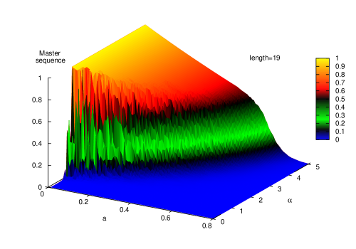
Figure 3: Simulation of the equilibrium density of the Master sequence

It is certainly well known that the population dynamics depends on the population size (see the discussion of Wilke [39]). In a theoretical study [28], Van Nimwegen, Crutchfield and Huynen developed a model for the evolution of populations on neutral networks and they show that an important parameter is the product of the population size and the mutation rate. The nature of the dynamics changes radically depending on whether this product is small or large. Sumedha, Martin and Peliti [35] analyze further the influence of this parameter. In [37], Van Nimwegen and Crutchfield derived analytical expressions for the waiting times needed to increase the fitness, starting from a local optimum. Their scaling relations involve the population size and show the existence of two different barriers, a fitness barrier and an entropy barrier. Although they pursue a different goal than ours, most of the heuristic ingredients explained previously are present in their work, and much more; they observe and discuss also the transition from the quasispecies regime for large populations to the disordered regime for small populations. The dependence on the population size and genome length has been investigated numerically by Elena, Wilke, Ofria and Lenski [15]. Here we show rigorously the existence of a critical population size for the sharp peak landscape in a specific asymptotic regime. The existence of a critical population size for the emergence of a quasispecies is a pleasing result: it shows that, even under the action of selection forces, a form of cooperation is necessary to create a quasispecies. Moreover the critical population size is much smaller than the cardinality of the possible genotypes. In conclusion, even in the very simple framework of the Moran model on the sharp peak landscape, cooperation is necessary to achieve the survival of the master sequence.

As emphasized by Eigen in [13], the error threshold phenomenon is similar to a phase transition in statistical mechanics. Leuthäusser established a formal correspondence between Eigen’s model and an anisotropic Ising model [24]. Several researchers have employed tools from statistical mechanics to analyze models of biological evolution, and more specifically the error threshold: see the nice review written by Baake and Gabriel [3]. Baake investigated the so–called Onsager landscape in [4]. This way she could transfer to a biological model the famous computation of Onsager for the two dimensional Ising model. Saakian, Deem and Hu [32] compute the variance of the mean fitness in a finite population model in order to control how it approximates the infinite population model. Deem, Muñoz and Park [31] use a field theoretic representation in order to derive analytical results.

We were also very much inspired by ideas from statistical mechanics, but with a different flavor. We do not use exact computations, rather we rely on softer tools, namely coupling techniques and correlation inequalities. These are the basic tools to prove the existence of a phase transition in classical models, like the Ising model or percolation. We seek large deviation estimates rather than precise scaling relations in our asymptotic regime. Of course the outcome of these techniques is very rough compared to exact computations, yet they are much more robust and their range of applicability is much wider. The model is presented in the next section and the main results in section 3. The remaining sections are devoted to the proofs. In the appendix we recall several classical results of the theory of finite Markov chains.

2 The model.

This section is devoted to the presentation of the model. Let $\cal A$ be a finite alphabet and let $\kappa=\text{card}\,\cal A$ be its cardinality. Let $\ell\geq 1$ be an integer. We consider the space ${\cal A}^{\ell}$ of sequences of length $\ell$ over the alphabet $\cal A$. Elements of this space represent the chromosome of an haploid individual, or equivalently its genotype. In our model, all the genes have the same set of alleles and each letter of the alphabet $\cal A$ is a possible allele. Typical examples are ${\cal A}=\{\,A,T,G,C\,\}$ to model standard DNA, or ${\cal A}=\{\,0,1\,\}$ to deal with binary sequences. Generic elements of ${\cal A}^{\ell}$ will be denoted by the letters $u,v,w$. We shall study a simple model for the evolution of a finite population of chromosomes on the space ${\cal A}^{\ell}$. An essential feature of the model we consider is that the size of the population is constant throughout the evolution. We denote by $m$ the size of the population. A population is an $m$–tuple of elements of ${\cal A}^{\ell}$. Generic populations will be denoted by the letters $x,y,z$. Thus a population $x$ is a vector

$$x\,=\,\left(\begin{matrix}x(1)\\ \vdots\\ x(m)\end{matrix}\right)$$

whose components are chromosomes. For $i\in\{\,1,\dots,m\,\}$, we denote by

$$x(i,1),\dots,x(i,\ell)$$

the letters of the sequence $x(i)$. This way a population $x$ can be represented as an array

$$x\,=\,\left(\begin{matrix}x(1,1)&\cdots&x(1,\ell)\\ \vdots&&\vdots\\ x(m,1)&\cdots&x(m,\ell)\\ \end{matrix}\right)$$

of size $m\times\ell$ of elements of $\cal A$, the $i$–th line being the $i$–th chromosome. The evolution of the population will be random and it will be driven by two antagonistic forces: mutation and replication.

Mutation. We assume that the mutation mechanism is the same for all the loci, and that mutations occur independently. Moreover we choose the most symmetric mutation scheme. We denote by $q\in]0,1-1/\kappa[$ the probability of the occurrence of a mutation at one particular locus. If a mutation occurs, then the letter is replaced randomly by another letter, chosen uniformly over the $\kappa-1$ remaining letters. We encode this mechanism in a mutation matrix

$$M(u,v)\,,\quad u,v\in{\cal A}^{\ell}$$

where $M(u,v)$ is the probability that the chromosome $u$ is transformed by mutation into the chromosome $v$. The analytical formula for $M(u,v)$ is then

$$M(u,v)\,=\,\prod_{j=1}^{\ell}\left((1-q){1}_{u(j)=v(j)}+\frac{q}{\kappa-1}{1}_{u(j)\neq v(j)}\right)\,.$$

Replication. The replication favors the development of fit chromosomes. The fitness of a chromosome is encoded in a fitness function

$$A:{\cal A}^{\ell}\to[0,+\infty[\,.$$

The fitness of a chromosome can be interpreted as its reproduction rate. A chromosome $u$ gives birth at random times and the mean time interval between two consecutive births is $1/A(u)$. In the context of Eigen’s model, the quantity $A(u)$ is the kinetic constant associated to the chemical reaction for the replication of a macromolecule of type $u$.

Authorized changes. In our model, the only authorized changes in the population consist in replacing one chromosome of the population by a new one. The new chromosome is obtained by replicating another chromosome, possibly with errors. We introduce a specific notation corresponding to these changes. For a population $x\in\smash{\left({\cal A}^{\ell}\right)^{m}}$, $j\in\{\,1,\dots,m\,\}$, $u\in{\cal A}^{\ell}$, we denote by $x(j\leftarrow u)$ the population $x$ in which the $j$–th chromosome $x(j)$ has been replaced by $u$:

$$x(j\leftarrow u)\,=\,\left(\begin{matrix}x(1)\\ \vdots\\ x(j-1)\\ u\\ x(j+1)\\ \vdots\\ x(m)\end{matrix}\right)$$

We make this modeling choice in order to build a very simple model. This type of model is in fact classical in population dynamics, they are called Moran models [16].

The mutation–replication scheme. Several further choices have to be done to define the model precisely. We have to decide how to combine the mutation and the replication processes. There exist two main schemes in the literature. In the first scheme, mutations occur at any time of the life cycle and they are caused by radiations or thermal fluctuations. This leads to a decoupled Moran model. In the second scheme, mutations occur at the same time as births and they are caused by replication errors. This is the case of the famous Eigen model and it leads to the Moran model we study here. This Moran model can be described loosely as follows. Births occur at random times. The rates of birth are given by the fitness function $A$. There is at most one birth at each instant. When an individual gives birth, it produces an offspring through a replication process. Errors in the replication process induce mutations. The offspring replaces an individual chosen randomly in the population (with the uniform probability).

We build next a mathematical model for the evolution of a finite population of size $m$ on the space ${\cal A}^{\ell}$, driven by mutation and replication as described above. We will end up with a stochastic process on the population space $\smash{\left({\cal A}^{\ell}\right)^{m}}$. Since the genetic composition of a population contains all the necessary information to describe its future evolution, our process will be Markovian.

Discrete versus continuous time. We can either build a discrete time Markov chain or a continuous time Markov process. Although the mathematical construction of a discrete time Markov chain is simpler, a continuous time process seems more adequate as a model of evolution for a population: births, deaths and mutations can occur at any time. In addition, the continuous time model is mathematically more appealing. We will build both types of models, in continuous and discrete time. Continuous time models are conveniently defined by their infinitesimal generators, while discrete time models are defined by their transition matrices (see the appendix). It should be noted, however, that the discrete time and the continuous time processes are linked through a standard stochastization procedure and they have the same stationary distribution. Therefore the asymptotic results we present here hold in both frameworks.

Infinitesimal generator. The continuous time Moran model is the Markov process $(X_{t})_{t\in{\mathbb{R}}^{+}}$ having the following infinitesimal generator: for $\phi$ a function from $\smash{\left({\cal A}^{\ell}\right)^{m}}$ to $\mathbb{R}$ and for any $x\in\smash{\left({\cal A}^{\ell}\right)^{m}}$,

$$\lim_{t\to 0}\,\frac{1}{t}\Big{(}E\big{(}\phi(X_{t})|X_{0}=x\big{)}-\phi(x)\Big{)}\,=\,\cr\sum_{1\leq i,j\leq m}\sum_{u\in{\cal A}^{\ell}}A(x(i))M(x(i),u)\Big{(}\phi\big{(}x(j\leftarrow u)\big{)}-\phi(x)\Big{)}\,.\hfil$$

Transition matrix. The discrete time Moran model is the Markov chain $(X_{n})_{n\in\mathbb{N}}$ whose transition matrix is given by

$$\forall n\in{\mathbb{N}}\quad\forall x\in\smash{\left({\cal A}^{\ell}\right)^{m}}\quad\forall j\in\{\,1,\dots,\ell\,\}\quad\forall u\in\smash{{\cal A}^{\ell}}\setminus\{\,x(j)\,\}\cr P\big{(}X_{n+1}=x(j\leftarrow u)\,|\,X_{n}=x\big{)}\,=\,\frac{1}{m^{2}\lambda}\sum_{1\leq i\leq m}{A(x(i))}M(x(i),u)\,,\hfil$$

where $\lambda>0$ is a constant such that

$$\lambda\,\geq\,\max\,\big{\{}\,A(u):{u\in\smash{{\cal A}^{\ell}}}\,\big{\}}\,.$$

The other non diagonal coefficients of the transition matrix are zero. The diagonal terms are chosen so that the sum of each line is equal to one. Notice that the continuous time formulation is more concise and elegant: it does not require the knowledge of the maximum of the fitness function $A$ in its definition.

Loose description of the dynamics. We explain first the discrete time dynamics of the Markov chain $(X_{n})_{n\in\mathbb{N}}$. Suppose that $X_{n}=x$ for some $n\in\mathbb{N}$ and let us describe loosely the transition mechanism to $X_{n+1}=y$. An index $i$ in $\{\,1,\dots,m\,\}$ is selected randomly with the uniform probability. With probability $1-{A(x(i))}/\lambda$, nothing happens and $y=x$. With probability ${A(x(i))}/{\lambda}$, the chromosome $x(i)$ enters the replication process and it produces an offspring $u$ according to the law $M(x(i),\cdot)$ given by the mutation matrix. Another index $j$ is selected randomly with uniform probability in $\{\,1,\dots,m\,\}$. The population $y$ is obtained by replacing the chromosome $x(j)$ in the population $x$ by a chromosome $u$.

We consider next the continuous time dynamics of the Markov process $(X_{t})_{t\in{\mathbb{R}}^{+}}$. The dynamics is governed by a clock that rings randomly. The time interval $\tau$ between each of the clock ringing is exponentially distributed with parameter $m^{2}{\lambda}$:

$$\forall t\in{\mathbb{R}}^{+}\qquad P(\tau>t)\,=\,\exp\big{(}-m^{2}{\lambda}t\big{)}\,.$$

Suppose that the clock rings at time $t$ and that the process was in state $x$ just before the time $t$. The population $x$ is transformed into the population $y$ following the same scheme as for the discrete time Markov chain $(X_{n})_{n\in\mathbb{N}}$ described previously. At time $t$, the process jumps to the state $y$.

3 Main results.

This section is devoted to the presentation of the main results.

Convention. The results hold for both the discrete time and the continuous time models, so we do not make separate statements. The time variable is denoted by $t$ throughout this section, it is either discrete with values in $\mathbb{N}$ or continuous with values in $\mathbb{R}^{+}$.

Sharp peak landscape. We will consider only the sharp peak landscape defined as follows. We fix a specific sequence, denoted by $w^{*}$, called the wild type or the master sequence. Let $\sigma>1$ be a fixed real number. The fitness function $A$ is given by

$$\forall u\in{\cal A}^{\ell}\qquad A(u)\,=\,\begin{cases}1&\text{if }u\neq w^{*}\\ \sigma&\text{if }u=w^{*}\\ \end{cases}$$

Density of the master sequence. We denote by $N(x)$ the number of copies of the master sequence $w^{*}$ present in the population $x$:

$$N(x)\,=\,\text{card}\,\big{\{}\,i:1\leq i\leq m,\,x(i)=w^{*}\,\big{\}}\,.$$

We are interested in the expected density of the master sequence in the steady state distribution of the process, that is,

$$\text{Master}(\sigma,\ell,m,q)\,=\,\lim_{t\to\infty}E\Big{(}\frac{1}{m}N(X_{t})\Big{)}\,,$$

as well as the variance

$$\text{Variance}(\sigma,\ell,m,q)\,=\,\lim_{t\to\infty}E\bigg{(}\Big{(}\frac{1}{m}N(X_{t})-\text{Master}(\sigma,\ell,m,q)\Big{)}^{2}\bigg{)}\,.$$

The limits exist because the transition mechanism of the Markov process $(X_{t})_{t\geq 0}$ is irreducible (and aperiodic for the discrete time case) as soon as the mutation probability is strictly between $0$ and $1$. Since the state space is finite, the Markov process $(X_{t})_{t\geq 0}$ admits a unique invariant probability measure, which describes the steady state of the process. The ergodic theorem for Markov chains implies that the law of $(X_{t})_{t\geq 0}$ converges towards this invariant probability measure, hence the above expectations converge. The limits depend on the parameters of the model, that is $\sigma,\ell,m,q$. Our choices for the infinitesimal generator and the matrix transition imply that the discrete time version and the continuous time version have exactly the same invariant probability measure. In order to exhibit a sharp transition phenomenon, we send $\ell,m$ to $\infty$ and $q$ to $0$. Let $\phi:{\mathbb{R}}^{+}\to{\mathbb{R}}^{+}\cup\{\,+\infty\,\}$ be the function defined by

$$\forall a<\ln\sigma\qquad\phi(a)\,=\,\frac{\displaystyle\sigma(1-e^{-a})\ln\frac{\displaystyle\sigma(1-e^{-a})}{\displaystyle\sigma-1}+\ln(\sigma e^{-a})}{\displaystyle(1-\sigma(1-e^{-a}))}$$

and $\phi(a)=0$ if $a\geq\ln\sigma$.

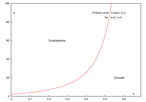
Figure 4: Critical curve

Theorem 3.1

We suppose that

$$\ell\to+\infty\,,\qquad m\to+\infty\,,\qquad q\to 0\,,$$

in such a way that

$${\ell q}\to a\in]0,+\infty[\,,\qquad\frac{m}{\ell}\to\alpha\in[0,+\infty]\,.$$

We have the following dichotomy:

$\bullet\quad$ If $\alpha\,\phi(a)<\ln\kappa$ then $\text{Master}\big{(}\sigma,\ell,m,q\big{)}\,\to\,0$.

$\bullet\quad$ If $\alpha\,\phi(a)>\ln\kappa$ then $\text{Master}\big{(}\sigma,\ell,m,q\big{)}\,\to\,\frac{\displaystyle\sigma e^{-a}-1}{\displaystyle\sigma-1}$.

In both cases, we have $\text{Variance}\big{(}\sigma,\ell,m,q\big{)}\,\to\,0$.

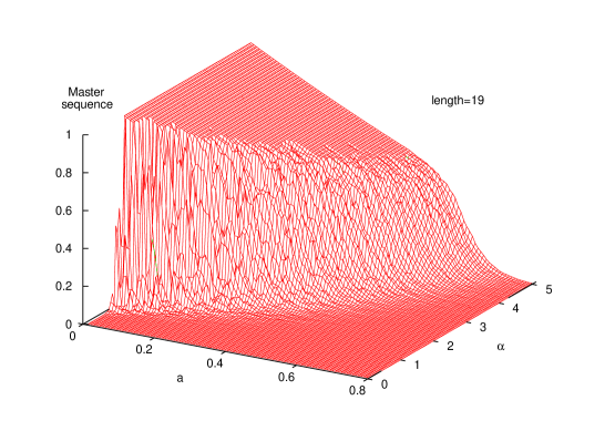
Figure 5: Master sequence at equilibrium

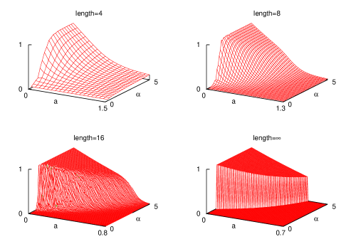
Figure 6: Varying the length $\ell$

These results are supported by computer simulations (see figure 5). On the simulations, which are of course done for small values of $\ell$, the transition associated to the critical population size seems even sharper than the transition associated to the error threshold. The programs are written in $C$ with the help of the GNU scientific library and the graphical output is generated with the help of the Gnuplot program. To increase the efficiency of the simulations, we simulated the occupancy process obtained by lumping the original Moran model. The number of generations in a simulation run was adjusted empirically in order to stabilize the output within a reasonable amount of time. Twenty years ago, Nowak and Schuster could perform simulations with $\ell=10$ and $m=100$ for $20\,000$ generations [30]. Today’s computer powers allow to simulate easily models with $\ell=20$ and $m=100$ for $10\,000\,000\,000$ generations. The good news is that, already for small values of $\ell$, the simulations are very conclusive. Figure 6 presents three pictures corresponding to simulations with $\ell=4,8,16$, as well as the theoretical shape for $\ell=\infty$ in the last picture. Notice that the statement of the theorem holds also in the case where $\alpha$ is null or infinite. This yields the following results:

Small populations. If $\ell,m\to+\infty,\,q\to 0,\,{\ell q}\to a\in]0,+\infty[,\,\frac{\textstyle m}{\textstyle\ell}\to 0$, then $\text{Master}\big{(}\sigma,\ell,m,q)\to 0$.

Large populations. Suppose that

$$\ell,m\to+\infty,\quad q\to 0,\quad{\ell q}\to a\in]0,+\infty[,\quad\frac{\textstyle m}{\textstyle\ell}\to+\infty\,.$$

If $a\geq\ln\sigma$, then $\text{Master}\big{(}\sigma,\ell,m,q)\to 0$. If $a<\ln\sigma$, then

$$\text{Master}\big{(}\sigma,\ell,m,q\big{)}\,\to\,\frac{\displaystyle\sigma e^{-a}-1}{\displaystyle\sigma-1}\,.$$

Interestingly, the large population regime is reminiscent of Eigen’s model. A slightly more restrictive formulation consists in sending $\ell$ to $\infty$, $m$ to $\infty$ and $q$ to $0$ in such a way that $m/\ell$ and $\ell q$ are kept constant. We might then take $q$ and $m$ as functions of $\ell$. Let $a,\alpha\in]0,+\infty[$. We take $q=a/\ell$ and $m=\alpha\ell$ and we have

$$\lim_{\ell\to\infty}\text{Master}\big{(}\sigma,\ell,\alpha\ell,a/\ell\big{)}\,=\,\begin{cases}\quad\phantom{aaa}0\phantom{\frac{1}{2}}&\text{if $\alpha\,\phi(a)<\ln\kappa$ }\\ \quad\displaystyle\frac{\displaystyle\sigma e^{-a}-1}{\displaystyle\sigma-1}\quad&\text{if $\alpha\,\phi(a)>\ln\kappa$ }\\ \end{cases}$$

Notice that $\alpha\,\phi(a)>\ln\kappa$ implies that $a<\ln\sigma$ and $\sigma e^{-a}>1$. The critical curve

$$\big{\{}\,(a,\alpha)\in{\mathbb{R}}^{+}\times{\mathbb{R}}^{+}:\alpha\,\phi(a)=\ln\kappa\,\big{\}}$$

corresponds to parameters $(a,\alpha)$ which are exactly at the error threshold and the critical population size. We are able to compute explicitly the critical curve and the limiting density because we consider a toy model. We did not examine here what happens on the critical curve. It is expected that the limiting density of the master sequence still fluctuates so that $\text{Variance}\big{(}\sigma,\ell,\alpha\ell,a/\ell\big{)}$ does not converge to $0$ whenever $\alpha\,\phi(a)=\ln\kappa$. An important observation is that the critical scaling should be the same for similar Moran models. In contrast, the critical curve seems to depend strongly on the specific dynamics of the model. However, in the limit where $a$ goes to $0$, the function $\phi(a)$ converges towards $\ln\sigma$. This yields the minimal population size allowing the emergence of a quasispecies.

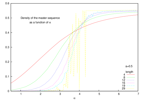
Figure 7: Critical population size

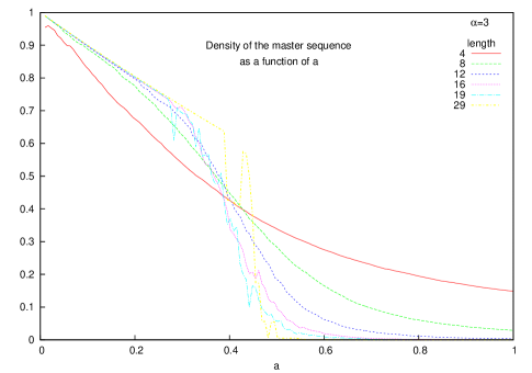
Figure 8: Error threshold

Corollary 3.2

If $\alpha<\ln\kappa/\ln\sigma$ then

$$\forall a>0\qquad\lim_{\ell\to\infty}\text{Master}\big{(}\sigma,\ell,\alpha\ell,a/\ell\big{)}\,=\,0\,.$$

If $\alpha>\ln\kappa/\ln\sigma$ then

$$\exists a>0\qquad\lim_{\ell\to\infty}\text{Master}\big{(}\sigma,\ell,\alpha\ell,a/\ell\big{)}\,>\,0\,.$$

We can also compute the maximal mutation rate permitting the emergence of a quasispecies. Interestingly, this maximal mutation rate is reminiscent of the error catastrophe in Eigen’s model.

Corollary 3.3

If $a>\ln\sigma$ then

$$\forall\alpha>0\qquad\lim_{\ell\to\infty}\text{Master}\big{(}\sigma,\ell,\alpha\ell,a/\ell\big{)}\,=\,0\,.$$

If $a<\ln\sigma$ then

$$\exists\alpha>0\qquad\lim_{\ell\to\infty}\text{Master}\big{(}\sigma,\ell,\alpha\ell,a/\ell\big{)}\,>\,0\,.$$

In conclusion, on the sharp peak landscape, a quasispecies can emerge only if

$$m\,>\,\frac{\ln\kappa}{\ln\sigma}\,\ell\,,\qquad q\,<\,\frac{\ln\sigma}{\ell}\,.$$

The heuristic ideas behind theorem 3.1 were explained in the introduction. These heuristics are quite simple, however, the corresponding proofs are rather delicate and technical. There is very little hope to do a proof entirely based on exact computations. Our strategy consists in comparing the original Moran process with simpler processes in order to derive adequate lower and upper bounds. To this end, we couple the various processes starting with different initial conditions (section 4). Unfortunately, the natural coupling for the Moran model we wish to study is not monotone. Therefore we consider an almost equivalent model, which we call the normalized Moran model. This model is obtained by normalizing the reproduction rates so that the total reproduction rate of any population is one (section 5). We first observe that the Moran model is exchangeable (section 6). However, the initial state space of the Moran process has no order structure and it is huge. We use a classical technique, called lumping, in order to reduce the state space (section 7). This way we obtain two lumped processes: the distance process $(D_{t})_{t\geq 0}$ which records the Hamming distances between the chromosomes of the population and the Master sequence and the occupancy process $(O_{t})_{t\geq 0}$ which records the distribution of these Hamming distances. The distance process is monotone in the neutral case $\sigma=1$, while the occupancy process is monotone for any value $\sigma\geq 1$ (section 8). Therefore we construct lower and upper processes to bound the occupancy process (section 9). These processes have the same dynamics as the original process in the neutral region and they evolve as a birth and death process as soon as the population contains a master sequence. We use then the ergodic theorem for Markov chains and a renewal argument to estimate the invariant probability measures of these processes. The behavior of the lower and upper bounds depends mainly on the persistence time and the discovery time of the master sequence. We rely on the explicit formulas available for birth and death processes to estimate the persistence time (section 10). To estimate the discovery time, we rely on rough estimates for the mutation dynamics and correlation inequalities (section 11). The mutation dynamics is quite similar to the Ehrenfest urn, however it is more complicated because several mutations can occur simultaneously and exact formulas are not available. The proof is concluded in section 12.

Warning. From section 6 onwards, we work with the normalized Moran model defined in section 5. This model is denoted by $(X_{t})_{t\geq 0}$ and its transition matrix by $p$, like the initial Moran model. We deal only with discrete time processes in the proofs. The time is denoted by $t$ or $n$.

4 Coupling

The definition of the processes through infinitesimal generator is not very intuitive at first sight. We will provide here a direct construction of the processes, which does not make appeal to a general existence result. This construction is standard and it is the formal counterpart of the loose description of the dynamics given in section 2. Moreover it provides a useful coupling of the processes with different initial conditions and different control parameters $\sigma,q$. All the processes will be built on a single large probability space. We consider a probability space $(\Omega,{\mathcal{F}},P)$ containing the following collection of independent random variables:

$\bullet$ a Poisson process $(\tau(t))_{t\geq 0}$ with intensity $m^{2}\lambda$.

$\bullet$ two sequences of random variables $I_{n},J_{n},\,n\geq 1$, with uniform law on the index set $\{\,1,\dots,\ell\,\}$.

$\bullet$ a family of random variables $U_{n,l},\,n\geq 1,\,1\leq l\leq\ell$, with uniform law on the interval $[0,1]$.

$\bullet$ a sequence of random variables $S_{n},\,n\geq 1$, with uniform law on the interval $[0,1]$.

We denote by $\tau_{n}$ the $n$–th arrival time of the Poisson process $(\tau(t))_{t\geq 0}$, i.e.,

$$\forall n\geq 1\qquad\tau_{n}\,=\,\inf\,\{\,t\geq 0:\tau(t)=n\,\}\,.$$

The random variables $I_{n}$, $J_{n}$, $U_{n,l},\,\,1\leq l\leq\ell$, and $S_{n}$ will be used to decide which move occurs at time $\tau_{n}$. To build the coupling, it is more convenient to replace the mutation probability $q$ by the parameter $p$ given by

$$p\,=\,\frac{\kappa}{\kappa-1}\,q\,.$$

We define a Markov chain $(X_{n})_{n\in\mathbb{N}}$ with the help of the previous random ingredients, whose law is the law of the Moran model. The process starts at time $0$ from an arbitrary population $x_{0}$. Let $n\geq 1$, suppose that the process has been defined up to time $n-1$ and that $X_{n-1}=x$. We explain how to build $X_{n}=y$. Let us set $i=I_{n}$. If $S_{n}>{A(x(i))}/{\lambda}$, then $y=x$. Suppose next that $S_{n}\leq{A(x(i))}/{\lambda}$. We define $y$ as follows. We index the elements of the alphabet $\mathcal{A}$ in an arbitrary way:

$${\mathcal{A}}\,=\,\big{\{}\,a_{1},\dots,a_{\kappa}\,\big{\}}\,.$$

Let $j=J_{n}$. We set

$$\forall l\in\{\,1,\dots,\ell\,\}\qquad y(j,l)\,=\,\begin{cases}\quad a_{1}&\text{if }\quad U_{n,l}<\genfrac{}{}{}{0}{p}{\kappa}\\ \quad\vdots\\ \quad a_{r}&\text{if }\quad(r-1)\genfrac{}{}{}{0}{p}{\kappa}<U_{n,l}<r\genfrac{}{}{}{0}{p}{\kappa}\\ \quad\vdots\\ \quad a_{\kappa}&\text{if }\quad(\kappa-1)\genfrac{}{}{}{0}{p}{\kappa}<U_{n,l}<p\\ \quad x(i,l)&\text{if }\quad U_{n,l}\geq p\\ \end{cases}$$

For $k\neq j$ we set $y(k)=x(k)$. Finally we define $X_{n}=y$.

We define also a Markov process $(X_{t})_{t\in\mathbb{R}^{+}}$ with right continuous trajectories. The process starts at time $0$ from an arbitrary population $x_{0}$ and it moves only when there is an arrival in the Poisson process $(\tau(t))_{t\geq 0}$. Let $t>0$ and suppose that $\tau_{n}=t$ for some $n\geq 1$. Suppose that just before $t$ the process was in state $x$:

$$\lim_{\genfrac{}{}{0.0pt}{1}{s\to t}{s<t}}X_{s}\,=\,x\,.$$

We proceed as in the construction of the discrete time process at step $n$ to build the new population $y$ starting from $x$ and we set $X_{t}=y$. Therefore we have

$$\forall n\geq 0\quad\forall t\in[\tau_{n},\tau_{n+1}[\qquad X_{t}\,=\,X_{n}\,.$$

5 Normalized model

The Moran model defined previously is difficult to analyze for several reasons. A major problem is that the natural coupling constructed in section 4 is not monotone. We define next a related Moran model which is simpler to study. This model is obtained by normalizing the reproduction rates so that the total reproduction rate of any population is one. The continuous time normalized Moran model is the Markov process $(X_{t})_{t\in{\mathbb{R}}^{+}}$ whose infinitesimal generator $L$ is defined as follows: for $\phi$ a function from $\smash{\left({\cal A}^{\ell}\right)^{m}}$ to $\mathbb{R}$ and for any $x\in\smash{\left({\cal A}^{\ell}\right)^{m}}$,

$$L\phi(x)\,=\,\sum_{1\leq i,j\leq m}\sum_{u\in{\cal A}^{\ell}}\frac{A(x(i))M(x(i),u)}{A(x(1))+\cdots+A(x(m))}\Big{(}\phi\big{(}x(j\leftarrow u)\big{)}-\phi(x)\Big{)}\,.$$

The discrete time normalized Moran model is the Markov chain $(X_{n})_{n\in\mathbb{N}}$ with transition matrix $p$ given by

$$\forall x\in\smash{\left({\cal A}^{\ell}\right)^{m}}\quad\forall j\in\{\,1,\dots,\ell\,\}\quad\forall u\in\smash{{\cal A}^{\ell}}\setminus\{\,x(j)\,\}\cr p\big{(}x,x(j\leftarrow u)\big{)}\,=\,\frac{1}{m}\sum_{1\leq i\leq m}\frac{A(x(i))M(x(i),u)}{A(x(1))+\cdots+A(x(m))}\,.$$

The other non diagonal coefficients of the transition matrix are zero. In the remaining of the paper, we shall work with this Markov chain $(X_{n})_{n\in\mathbb{N}}$ and the transition matrix $p$. We shall prove the main theorem 3.1 of section 3 for this process. In fact, we shall even prove the following stronger result. Let $\nu$ be the image of the invariant probability measure of $(X_{n})_{n\geq 0}$ through the map

$$x\in\big{(}{\mathcal{A}}^{\ell}\big{)}^{m}\mapsto\frac{1}{m}N(x)\in[0,1]\,.$$

The probability measure $\nu$ is a measure on the interval $[0,1]$ describing the equilibrium density of the master sequence in the population. Indeed,

$$\forall i\in\{\,0,\dots,m\,\}\qquad\nu\Big{(}\frac{i}{m}\Big{)}\,=\,\lim_{n\to\infty}\,P\big{(}N(X_{n})=i\big{)}\,.$$

The probability $\nu$ depends on the parameters $\sigma,\ell,m,q$ of the model. Let $\phi(a)$ be the function defined before theorem 3.1, i.e.,

$$\forall a<\ln\sigma\qquad\phi(a)\,=\,\frac{\displaystyle\sigma(1-e^{-a})\ln\frac{\displaystyle\sigma(1-e^{-a})}{\displaystyle\sigma-1}+\ln(\sigma e^{-a})}{\displaystyle(1-\sigma(1-e^{-a}))}$$

and $\phi(a)=0$ if $a\geq\ln\sigma$. Let

$$\rho^{*}\,=\,\frac{\displaystyle\sigma e^{-a}-1}{\displaystyle\sigma-1}\,.$$

Theorem 5.1

We suppose that

$$\ell\to+\infty\,,\qquad m\to+\infty\,,\qquad q\to 0\,,$$

in such a way that

$${\ell q}\to a\in]0,+\infty[\,,\qquad\frac{m}{\ell}\to\alpha\in[0,+\infty]\,.$$

We have the following dichotomy:

$\bullet\quad$ If $\alpha\,\phi(a)<\ln\kappa$ then $\nu$ converges towards the Dirac mass at $0$:

$$\forall\varepsilon>0\qquad\nu([0,\varepsilon])\,\to\,1\,.$$

$\bullet\quad$ If $\alpha\,\phi(a)>\ln\kappa$ then $\nu$ converges towards the Dirac mass at $\rho^{*}$:

$$\forall\varepsilon>0\qquad\nu([\rho^{*}-\varepsilon,\rho^{*}+\varepsilon])\,\to\,1\,.$$

We shall prove this theorem for the normalized Moran model $(X_{n})_{n\in\mathbb{N}}$. Let us show how this implies theorem 3.1 for the initial model. In the remainder of this argument, we denote by $(X^{\prime}_{n})_{n\in\mathbb{N}}$ the Moran model described in section 2 and by $p^{\prime}$ its transition matrix. The transition matrices $p$ and $p^{\prime}$ are related by the simple relation

$$\forall x,y\in\big{(}{\mathcal{A}}^{\ell}\big{)}^{m}\,,\quad x\neq y\,,\qquad p^{\prime}(x,y)\,=\,\beta(x)\,p(x,y)$$

where

$$\forall x\in\big{(}{\mathcal{A}}^{\ell}\big{)}^{m}\qquad\beta(x)\,=\,\frac{1}{m\lambda}\big{(}{A(x(1))+\cdots+A(x(m))\big{)}}\,.$$

Let $\mu$ and $\mu^{\prime}$ be the invariant probability measures of the processes $(X_{t})_{t\geq 0}$ and $(X^{\prime}_{t})_{t\geq 0}$. The probability $\mu$ is the unique solution of the system of equations

$$\forall x\in\big{(}{\mathcal{A}}^{\ell}\big{)}^{m}\qquad\mu(x)\,=\,\sum_{y\in({\mathcal{A}}^{\ell})^{m}}{\mu(y)}\,p(y,x)\,.$$

We rewrite these equations as:

$$\forall x\in\big{(}{\mathcal{A}}^{\ell}\big{)}^{m}\qquad\mu(x)\sum_{\genfrac{}{}{0.0pt}{1}{y\in({\mathcal{A}}^{\ell})^{m}}{y\neq x}}\,p(x,y)\,=\,\sum_{\genfrac{}{}{0.0pt}{1}{y\in({\mathcal{A}}^{\ell})^{m}}{y\neq x}}{\mu(y)}\,p(y,x)\,.$$

Replacing $p$ by $p^{\prime}$, we get

$$\forall x\in\big{(}{\mathcal{A}}^{\ell}\big{)}^{m}\qquad\frac{\mu(x)}{\beta(x)}\sum_{\genfrac{}{}{0.0pt}{1}{y\in({\mathcal{A}}^{\ell})^{m}}{y\neq x}}\,p^{\prime}(x,y)\,=\,\sum_{\genfrac{}{}{0.0pt}{1}{y\in({\mathcal{A}}^{\ell})^{m}}{y\neq x}}\frac{\mu(y)}{\beta(y)}\,p^{\prime}(y,x)\,.$$

Using the uniqueness of the invariant probability measure associated to $p^{\prime}$, we conclude that

$$\forall x\in\big{(}{\mathcal{A}}^{\ell}\big{)}^{m}\qquad\mu^{\prime}(x)\,=\,\frac{\displaystyle\frac{\mu(x)}{\beta(x)}}{\displaystyle\sum_{y\in({\mathcal{A}}^{\ell})^{m}}\frac{\mu(y)}{\beta(y)}}\,.$$

In the case of the sharp peak landscape, the function $\beta(x)$ can be rewritten as

$$\forall x\in\big{(}{\mathcal{A}}^{\ell}\big{)}^{m}\qquad\beta(x)\,=\,\frac{1}{m\lambda}\big{(}(\sigma-1)N(x)+m\big{)}\,.$$

Let us denote by $\nu$ and $\nu^{\prime}$ the images of $\mu$ and $\mu^{\prime}$ through the map

$$x\in\big{(}{\mathcal{A}}^{\ell}\big{)}^{m}\mapsto\frac{1}{m}N(x)\in[0,1]\,.$$

We can thus rewrite

$$\sum_{y\in({\mathcal{A}}^{\ell})^{m}}\frac{\mu(y)}{\beta(y)}\,=\,\sum_{y\in({\mathcal{A}}^{\ell})^{m}}\frac{\displaystyle\lambda{\mu(y)}}{\displaystyle(\sigma-1)\frac{N(y)}{m}+1}\,=\,\int_{[0,1]}\frac{\displaystyle\lambda\,d\nu(t)}{\displaystyle(\sigma-1)t+1}\,.$$

For any function $f:[0,1]\to{\mathbb{R}}$, we have then

$$\int_{[0,1]}f\,d\nu^{\prime}\,=\,\lim_{t\to\infty}E\bigg{(}f\Big{(}\frac{1}{m}N(X^{\prime}_{t})\Big{)}\bigg{)}\,=\,\sum_{x\in({\mathcal{A}}^{\ell})^{m}}f\Big{(}\frac{1}{m}N(x)\Big{)}\,\mu^{\prime}(x)\cr\,=\,\frac{\displaystyle\sum_{x\in({\mathcal{A}}^{\ell})^{m}}f\Big{(}\frac{N(x)}{m}\Big{)}\frac{\mu(x)}{\beta(x)}}{\displaystyle\sum_{y\in({\mathcal{A}}^{\ell})^{m}}\frac{\mu(y)}{\beta(y)}}\,=\,\frac{\displaystyle\int_{[0,1]}\frac{\displaystyle\lambda f(t)\,d\nu(t)}{\displaystyle(\sigma-1)t+1}}{\displaystyle\int_{[0,1]}\frac{\displaystyle\lambda\,d\nu(t)}{\displaystyle(\sigma-1)t+1}}\,.$$

We suppose that

$$\ell\to+\infty\,,\qquad m\to+\infty\,,\qquad q\to 0\,,$$

in such a way that

$${\ell q}\to a\in]0,+\infty[\,,\qquad\frac{m}{\ell}\to\alpha\in[0,+\infty]\,.$$

By theorem 5.1, away from the critical curve $\alpha\,\phi(a)=\ln\kappa$, the probability $\nu$ converges towards a Dirac mass. If $\nu$ converges towards a Dirac mass at $\rho$, then we conclude from the above formula that $\nu^{\prime}$ converges towards the same Dirac mass and

$$\text{Master}\big{(}\sigma,\ell,m,q\big{)}\, \to\,\rho\,,\qquad$$

$$\text{Variance}\big{(}\sigma,\ell,m,q\big{)}\, \to\,0\,.$$

This way we obtain the statements of theorem 3.1. From now onwards, in the proofs, we work exclusively with the normalized Moran process, and we denote it by $(X_{t})_{t\geq 0}$.

6 Exchangeability

The symmetric group $\mathfrak{S}_{m}$ of the permutations of $\{\,1,\dots,m\,\}$ acts in a natural way on the populations through the following group operation:

$$\forall x\in\big{(}{\mathcal{A}}^{\ell}\big{)}^{m}\quad\forall\rho\in\mathfrak{S}_{m}\quad\forall j\in\{\,1,\dots,m\,\}\qquad(\rho\cdot x)(j)\,=\,x(\rho(j))\,.$$

A probability measure $\mu$ on $\big{(}{\mathcal{A}}^{\ell}\big{)}^{m}$ is exchangeable if it is invariant under the action of $\mathfrak{S}_{m}$:

$$\forall\rho\in\mathfrak{S}_{m}\quad\forall x\in\big{(}{\mathcal{A}}^{\ell}\big{)}^{m}\quad\mu(\rho\cdot x)\,=\,\mu(x)\,.$$

A process $(X_{t})_{t\geq 0}$ with values in $\big{(}{\mathcal{A}}^{\ell}\big{)}^{m}$ is exchangeable if and only if, for any $t\geq 0$, the law of $X_{t}$ is exchangeable.

Lemma 6.1

The transition matrix $p$ is invariant under the action of $\mathfrak{S}_{m}$:

$$\forall x\in\big{(}{\mathcal{A}}^{\ell}\big{)}^{m}\quad\forall\rho\in\mathfrak{S}_{m}\quad\forall j\in\{\,1,\dots,m\,\}\quad\forall u\in\smash{{\cal A}^{\ell}}\setminus\{\,x(j)\,\}\cr p\big{(}\rho\cdot x,\rho\cdot(x(j\leftarrow u))\big{)}\,=\,p\big{(}x,x(j\leftarrow u)\big{)}\,.$$

Proof.

Let $x,\rho,j,u$ be as in the statement of the lemma. We have

$$p\big{(}\rho\cdot x,\rho\cdot(x(j\leftarrow u))\big{)}\,=\,p\big{(}\rho\cdot x,(\rho\cdot x)(\rho^{-1}(j)\leftarrow u)\big{)}\cr\,=\,\frac{1}{m}\sum_{1\leq i\leq m}\frac{A((\rho\cdot x)(i))M((\rho\cdot x)(i),u)}{A((\rho\cdot x)(1))+\cdots+A((\rho\cdot x)(m))}\cr\,=\,\frac{1}{m}\sum_{1\leq i\leq m}\frac{A(x(i))M(x(i),u)}{A(x(1))+\cdots+A(x(m))}\,=\,p\big{(}x,x(j\leftarrow u)\big{)}\,.$$

Thus the matrix $p$ satisfies the required invariance property. □

Corollary 6.2

Let $\mu$ be an exchangeable probability distribution on the population space $\big{(}{\mathcal{A}}^{\ell}\big{)}^{m}$. The Moran model $(X_{t})_{t\geq 0}$ starting with $\mu$ as the initial distribution is exchangeable.

Proof.

Let $\rho\in\mathfrak{S}_{m}$ and let $f$ be a function from $\big{(}{\mathcal{A}}^{\ell}\big{)}^{m}$ to ${\mathbb{R}}$. Using the exchangeability of $\mu$ and lemma 6.1, we have, for any $t\geq 1$,

$$E\big{(}f(\rho\cdot X_{t})\big{)}\,=\,\sum_{x_{0},\cdots,x_{t}\in({\mathcal{A}}^{\ell})^{m}}\mu(x_{0})\,p(x_{0},x_{1})\cdots p(x_{t-1},x_{t})\,f(\rho\cdot X_{t})\cr\sum_{x_{0},\cdots,x_{t}\in({\mathcal{A}}^{\ell})^{m}}\mu(\rho\cdot x_{0})\,p(\rho\cdot x_{0},\rho\cdot x_{1})\cdots p(\rho\cdot x_{t-1},\rho\cdot x_{t})\,f(\rho\cdot X_{t})\cr\,=\,\sum_{x_{0},\cdots,x_{t}\in({\mathcal{A}}^{\ell})^{m}}\mu(x_{0})\,p(x_{0},x_{1})\cdots p(x_{t-1},x_{t})\,f(X_{t})\,=\,E\big{(}f(X_{t})\big{)}\,.$$

Thus the process $(X_{t})_{t\geq 0}$ is exchangeable. □

7 Lumping

The state space of the process $(X_{t})_{t\geq 0}$ is huge, it has cardinality $\kappa^{\ell m}$. We will rely on a classical technique to reduce the state space called lumping (see the appendix). We consider here only the sharp peak landscape. In this situation, the fitness of a chromosome is a function of its distance to the master sequence. A close look at the mutation mechanism reveals that chromosomes which are at the same distance from the Master sequence are equivalent for the dynamics, hence they can be lumped together in order to build a simpler process on a reduced space. For simplicity, we consider only the discrete time process. However similar results hold in continuous time.

7.1 Distance process

We denote by $d_{H}$ the Hamming distance between two chromosomes:

$$\forall u,v\in{\mathcal{A}}^{\ell}\qquad d_{H}(u,v)\,=\,\text{card}\,\,\big{\{}\,j:1\leq j\leq\ell,\,u(j)\neq v(j)\,\big{\}}\,.$$

We will keep track of the distances of the chromosomes to the master sequence $w^{*}$. We define a function ${H}:\smash{{\cal A}^{\ell}}\to\{\,0,\dots,\ell\,\}$ by setting

$$\forall u\in{\cal A}^{\ell}\qquad H(u)\,=\,d_{H}\big{(}u,w^{*}\big{)}\,.$$

The map $H$ induces a partition of ${\cal A}^{\ell}$ into Hamming classes

$$H^{-1}(\{\,b\,\})\,,\qquad b\in\{\,0,\dots,\ell\,\}\,.$$

We prove first that the mutation matrix is lumpable with respect to the function $H$.

Lemma 7.1 (Lumped mutation matrix)

Let $b,c\in\{\,0,\dots,\ell\,\}$ and let $u\in{\mathcal{A}}^{\ell}$ such that $H(u)=b$. The sum

$$\sum_{\genfrac{}{}{0.0pt}{1}{w\in{{\cal A}^{\ell}}}{H(w)=c}}M(u,w)$$

does not depend on $u$ in $H^{-1}(\{\,b\,\})$, it is a function of $b$ and $c$ only, which we denote by $M_{H}(b,c)$. The coefficient $M_{H}(b,c)$ is equal to

$$\sum_{\genfrac{}{}{0.0pt}{1}{0\leq k\leq\ell-b}{\genfrac{}{}{0.0pt}{1}{0\leq l\leq b}{k-l=c-b}}}{\binom{\ell-b}{k}}{\binom{b}{l}}\Big{(}p\Big{(}1-\frac{1}{\kappa}\Big{)}\Big{)}^{k}\Big{(}1-p\Big{(}1-\frac{1}{\kappa}\Big{)}\Big{)}^{\ell-b-k}\Big{(}\frac{p}{\kappa}\Big{)}^{l}\Big{(}1-\frac{p}{\kappa}\Big{)}^{b-l}\,.$$

Proof.

Let $b,c\in\{\,0,\dots,\ell\,\}$ and let $u\in{\mathcal{A}}^{\ell}$ such that $H(u)=b$. We will compute the law of $H(w)$ whenever $w$ follows the law $M(u,\cdot)$ given by the line of $M$ associated to $u$. For any $w\in{\mathcal{A}}^{\ell}$, we have

$$H(w)\,=\,\sum_{1\leq l\leq\ell}1_{w(l)\neq w^{*}(l)}\cr\,=\,\sum_{1\leq l\leq\ell}\Big{(}1_{w(l)\neq w^{*}(l),u(l)=w^{*}(l)}+1_{w(l)\neq w^{*}(l),u(l)\neq w^{*}(l)}\Big{)}\cr\,=\,H(u)+\sum_{1\leq l\leq\ell}\Big{(}1_{w(l)\neq w^{*}(l),u(l)=w^{*}(l)}-1_{w(l)=w^{*}(l),u(l)\neq w^{*}(l)}\Big{)}\,.$$

According to the mutation kernel $M$, for indices $l$ such that $u(l)=w^{*}(l)$, the variable $\smash{1_{w(l)\neq w^{*}(l)}}$ is Bernoulli with parameter $p(1-1/\kappa)$, while for indices $l$ such that $u(l)\neq w^{*}(l)$, the variable $1_{w(l)=w^{*}(l)}$ is Bernoulli with parameter $p/\kappa$. Moreover these Bernoulli variables are independent. Thus the law of $H(w)$ under the kernel $M(u,w)$ is given by

$$H(u)+\text{Binomial}\big{(}\ell-H(u),p(1-1/\kappa)\big{)}-\text{Binomial}\big{(}H(u),p/\kappa\big{)}$$

where the two binomial random variables are independent. This law depends only on $H(u)$, therefore the sum

$$\sum_{\genfrac{}{}{0.0pt}{1}{w\in{{\cal A}^{\ell}}}{H(w)=c}}M(u,w)$$

is a function of $b=H(u)$ and $c=H(w)$ only, which we denote by $M_{H}(b,c)$. The formula for the lumped matrix $M_{H}$ is obtained by computing the law of the difference of the two independent binomial laws appearing above. □

The fitness function $A$ of the sharp peak landscape can be factorized through $H$. If we define

$$\forall b\in\{\,0,\dots,\ell\,\}\qquad A_{H}(b)\,=\,\begin{cases}\sigma&\text{if }b=0\\ 1&\text{if }b\geq 1\\ \end{cases}$$

then we have

$$\forall u\in{\cal A}^{\ell}\qquad A(u)\,=\,A_{H}(H(u))\,.$$

We define further a vector function ${\mathbb{H}}:{\left({\cal A}^{\ell}\right)^{m}}\to\{\,0,\dots,\ell\,\}^{m}$ by setting

$$\forall x\,=\,\left(\begin{matrix}x(1)\\ \vdots\\ x(m)\end{matrix}\right)\in\smash{\left({\cal A}^{\ell}\right)^{m}}\qquad{\mathbb{H}}(x)\,=\,\left(\begin{matrix}H\big{(}x(1)\big{)}\\ \vdots\\ H\big{(}x(m)\big{)}\end{matrix}\right)\,.$$

The partition of $\smash{\left({\cal A}^{\ell}\right)^{m}}$ induced by the map $\mathbb{H}$ is

$${\mathbb{H}}^{-1}(\{\,d\,\})\,,\qquad d\in\{\,0,\dots,\ell\,\}^{m}\,.$$

We define finally the distance process $(D_{t})_{t\geq 0}$ by

$$\forall t\geq 0\qquad D_{t}\,=\,{\mathbb{H}}\big{(}X_{t}\big{)}\,.$$

Our next goal is to prove that the process $(X_{t})_{t\geq 0}$ is lumpable with respect to the partition of $\smash{\left({\cal A}^{\ell}\right)^{m}}$ induced by the map $\mathbb{H}$, so that the distance process $(D_{t})_{t\geq 0}$ is a genuine Markov process.

Proposition 7.2 (${\mathbb{H}}$ Lumpability)

Let $p$ be the transition matrix of the Moran model. We have

$$\forall e\in\{\,0,\dots,\ell\,\}^{m}\quad\forall x,y\in{\left({\cal A}^{\ell}\right)^{m}}\,,\cr{\mathbb{H}}(x)={\mathbb{H}}(y)\quad\Longrightarrow\quad\sum_{\genfrac{}{}{0.0pt}{1}{z\in{\left({\cal A}^{\ell}\right)^{m}}}{{\mathbb{H}}(z)=e}}p(x,z)\,=\,\sum_{\genfrac{}{}{0.0pt}{1}{z\in{\left({\cal A}^{\ell}\right)^{m}}}{{\mathbb{H}}(z)=e}}p(y,z)\,.$$

Proof.

For the process $(X_{t})_{t\geq 0}$, the only transitions having positive probability are the transitions of the form

$$x\quad\longrightarrow\quad x(j\leftarrow u)\,,\qquad 1\leq j\leq m,\quad u\in{\mathcal{A}}^{\ell}\,.$$

Let $e\in\{\,0,\dots,\ell\,\}^{m}$ and let $x,y\in{\left({\cal A}^{\ell}\right)^{m}}$ be such that ${\mathbb{H}}(x)={\mathbb{H}}(y)$. We set $d={\mathbb{H}}(x)={\mathbb{H}}(y)$. If the vectors $d,e$ differ for more than two components, then the sums appearing in the statement of the proposition are equal to zero. Suppose first that the vectors $d,e$ differ in exactly one component, so that there exist $j\in\{\,1,\dots,m\,\}$ and $c\in\{\,0,\dots,\ell\,\}$ such that $e=d(j\leftarrow c)$ and $d(j)\neq c$. Naturally, $d(j\leftarrow c)$ is the vector $d$ in which the $j$–th component $d(j)$ has been replaced by $c$:

$$d(j\leftarrow c)\,=\,\left(\begin{matrix}d(1)\\ \vdots\\ d(j-1)\\ c\\ d(j+1)\\ \vdots\\ d(m)\end{matrix}\right)$$

We have then

$$\sum_{\genfrac{}{}{0.0pt}{1}{z\in{\left({\cal A}^{\ell}\right)^{m}}}{{\mathbb{H}}(z)=e}}p(x,z)\,=\,\sum_{\genfrac{}{}{0.0pt}{1}{w\in{{\cal A}^{\ell}}}{H(w)=c}}p\big{(}x,x(j\leftarrow w)\big{)}\,.$$

Using lemma 7.1, we have

$$\sum_{\genfrac{}{}{0.0pt}{1}{w\in{{\cal A}^{\ell}}}{H(w)=c}}p\big{(}x,x(j\leftarrow w)\big{)}\,=\,\sum_{\genfrac{}{}{0.0pt}{1}{w\in{{\cal A}^{\ell}}}{H(w)=c}}\frac{1}{m}\sum_{1\leq i\leq m}\frac{A(x(i))M(x(i),w)}{A(x(1))+\cdots+A(x(m))}\cr\,=\,\frac{1}{m}\sum_{1\leq i\leq m}\frac{{{A_{H}\big{(}H(x(i))\big{)}}M_{H}(H(x(i)),c)}}{A_{H}\big{(}H(x(1))\big{)}+\cdots+A_{H}\big{(}H(x(m))\big{)}}\,.$$

This sum is a function of ${\mathbb{H}}(x)$ and $c$ only. Since ${\mathbb{H}}(x)={\mathbb{H}}(y)$, the sums are the same for $x$ and $y$. Suppose next that $d=e$. Then

$$\sum_{\genfrac{}{}{0.0pt}{1}{z\in{\left({\cal A}^{\ell}\right)^{m}}}{{\mathbb{H}}(z)=e}}p(x,z)\,=\,p(x,x)\,+\,\sum_{1\leq j\leq m}\sum_{\genfrac{}{}{0.0pt}{1}{w\in{{\cal A}^{\ell}\setminus\{\,x(j)\,\}}}{H(w)=H(x(j))}}p\big{(}x,x(j\leftarrow w)\big{)}\cr\,=\,1-\kern-7.0pt\sum_{\genfrac{}{}{0.0pt}{1}{1\leq j\leq m}{w\in{{\cal A}^{\ell}\setminus\{\,x(j)\,\}}}}\kern-7.0ptp\big{(}x,x(j\leftarrow w)\big{)}+\sum_{1\leq j\leq m}\sum_{\genfrac{}{}{0.0pt}{1}{w\in{{\cal A}^{\ell}\setminus\{\,x(j)\,\}}}{H(w)=H(x(j))}}p\big{(}x,x(j\leftarrow w)\big{)}\cr\,=\,1-\sum_{1\leq j\leq m}\sum_{\genfrac{}{}{0.0pt}{1}{w\in{{\cal A}^{\ell}\setminus\{\,x(j)\,\}}}{H(w)\neq H(x(j))}}p\big{(}x,x(j\leftarrow w)\big{)}\cr\,=\,1-\sum_{1\leq j\leq m}\sum_{\genfrac{}{}{0.0pt}{1}{c\in\{\,0,\dots,\ell\,\}}{c\neq H(x(j))}}\sum_{\genfrac{}{}{0.0pt}{1}{w\in{{\cal A}^{\ell}}}{H(w)=c}}p\big{(}x,x(j\leftarrow w)\big{)}\,.$$

We have seen in the previous case that the last sum is a function of ${\mathbb{H}}(x)$ and $c$ only. The second sum as well depends only on ${\mathbb{H}}(x)$. Therefore the above quantity is the same for $x$ and $y$. □

We apply the classical lumping result (see theorem A.3) to conclude that the distance process $(D_{t})_{t\geq 0}$ is a Markov process. From the previous computations, we see that its transition matrix $p_{H}$ is given by

$$\forall d\in\{\,0,\dots,\ell\,\}^{m}\quad\forall j\in\{\,1,\dots,m\,\}\quad\forall c\in\{\,0,\dots,\ell\,\}\setminus\{\,d(j)\,\}\cr p_{H}\big{(}d,d(j\leftarrow c)\big{)}\,=\,\frac{1}{m}\sum_{1\leq i\leq m}\frac{{{A_{H}(d(i))}M_{H}(d(i),c)}}{A_{H}(d(1))+\cdots+A_{H}(d(m))}\,.$$

7.2 Occupancy process

We denote by ${\mathcal{P}}^{m}_{\ell+1}$ the set of the ordered partitions of the integer $m$ in at most $\ell+1$ parts:

$${\mathcal{P}}^{m}_{\ell+1}\,=\,\big{\{}\,(o(0),\dots,o(\ell))\in{\mathbb{N}}^{\ell+1}:o(0)+\cdots+o(\ell)=m\,\big{\}}\,.$$

These partitions are interpreted as occupancy distributions. The partition $(o(0),\dots,o(\ell))$ corresponds to a population in which $o(l)$ chromosomes are at Hamming distance $l$ from the master sequence, for any $l\in\{\,0,\dots,\ell\,\}$. Let $\mathcal{O}$ be the map which associates to each population $x$ its occupancy distribution ${\mathcal{O}}(x)=(o(x,0),\dots,o(x,\ell))$, defined by:

$$\forall l\in\{\,0,\dots,\ell\,\}\qquad o(x,l)\,=\,\text{card}\,\big{\{}\,i:1\leq i\leq m,\,d_{H}(x(i),w^{*})=l\,\big{\}}\,.$$

The map ${\cal O}$ can be factorized through ${\mathbb{H}}$. For $d\in\{\,0,\dots,\ell\,\}^{m}$, we set

$$o_{H}(d,l)\,=\,\text{card}\,\big{\{}\,i:1\leq i\leq m,\,d(i)=l\,\big{\}}$$

and we define a map ${\cal O}_{H}:\{\,0,\dots,\ell\,\}^{m}\to{\mathcal{P}}^{m}_{\ell+1}$ by setting

$${\cal O}_{H}(d)\,=\,(o_{H}(d,0),\dots,o_{H}(d,\ell))\,.$$

We have then

$$\forall x\in\big{(}{\mathcal{A}}^{\ell}\big{)}^{m}\qquad{\cal O}(x)\,=\,{\cal O}_{H}\big{(}{\mathbb{H}}(x)\big{)}\,.$$

The map ${\cal O}$ lumps together populations which are permutations of each other:

$$\forall x\in\big{(}{\mathcal{A}}^{\ell}\big{)}^{m}\quad\forall\rho\in\mathfrak{S}_{m}\qquad{\cal O}(x)\,=\,{\cal O}(\rho\cdot x)\,.$$

We define the occupancy process $(O_{t})_{t\geq 0}$ by setting

$$\forall t\geq 0\qquad O_{t}\,=\,{\mathcal{O}}(X_{t})\,=\,{\mathcal{O}}_{H}(D_{t})\,.$$

For the process $(D_{t})_{t\geq 0}$, the only transitions having positive probability are the transitions of the form

$$d\quad\longrightarrow\quad d(j\leftarrow c)\,,\qquad 1\leq j\leq m,\quad c\in\{\,0,\dots,\ell\,\}\,.$$

Therefore the only possible transitions for the process $(O_{t})_{t\geq 0}$ are

$$o\quad\longrightarrow\quad o(k\rightarrow l)\,,\qquad 0\leq k,l\leq\ell\,,$$

where $o(k\rightarrow l)$ is the partition obtained by moving a chromosome from the class $k$ to the class $l$, i.e.,

$$\forall h\in\{\,0,\dots,\ell\,\}\qquad o(k\rightarrow l)(h)\,=\,\begin{cases}o(h)&\text{if }h\neq k,l\\ o(k)-1&\text{if }h=k\\ o(l)+1&\text{if }h=l\\ \end{cases}$$

Proposition 7.3 (${\mathcal{O}}$ Lumpability)

Let $p_{H}$ be the transition matrix of the distance process. We have

$$\forall o\in{\mathcal{P}}^{m}_{\ell+1}\quad\forall d,e\in\{\,0,\dots,\ell\,\}^{m}\,,\cr{\mathcal{O}}_{H}(d)={\mathcal{O}}_{H}(e)\quad\Longrightarrow\quad\sum_{\genfrac{}{}{0.0pt}{1}{f\in\{\,0,\dots,\ell\,\}^{m}}{{\mathcal{O}}_{H}(f)=o}}p_{H}(d,f)\,=\,\sum_{\genfrac{}{}{0.0pt}{1}{f\in\{\,0,\dots,\ell\,\}^{m}}{{\mathcal{O}}_{H}(f)=o}}p_{H}(e,f)\,.$$

Proof.

Let $o\in{\mathcal{P}}^{m}_{\ell+1}$ and $d,e\in\{\,0,\dots,\ell\,\}^{m}$ such that ${{\mathcal{O}}_{H}(d)={\mathcal{O}}_{H}(e)}$. Since ${\mathcal{O}}_{H}(d)={\mathcal{O}}_{H}(e)$, then there exists a permutation $\rho\in\mathfrak{S}_{m}$ such that $\rho\cdot d=e$. By lemma 6.1, the transition matrices $p$ and $p_{H}$ are invariant under the action of $\mathfrak{S}_{m}$, therefore

$$\sum_{\genfrac{}{}{0.0pt}{1}{f\in\{\,0,\dots,\ell\,\}^{m}}{{\mathcal{O}}_{H}(f)=o}}p_{H}(d,f)\,=\,\sum_{\genfrac{}{}{0.0pt}{1}{f\in\{\,0,\dots,\ell\,\}^{m}}{{\mathcal{O}}_{H}(f)=o}}p_{H}(\rho\cdot d,\rho\cdot f)\cr\,=\,\sum_{\genfrac{}{}{0.0pt}{1}{f\in\{\,0,\dots,\ell\,\}^{m}}{{\mathcal{O}}_{H}(\rho^{-1}\cdot f)=o}}p_{H}(e,f)\,=\,\sum_{\genfrac{}{}{0.0pt}{1}{f\in\{\,0,\dots,\ell\,\}^{m}}{{\mathcal{O}}_{H}(f)=o}}p_{H}(e,f)$$

as requested. □

We apply the classical lumping result (see theorem A.3) to conclude that the occupancy process $(O_{t})_{t\geq 0}$ is a Markov process. Let us compute its transition probabilities. Let $o\in{\mathcal{P}}^{m}_{\ell+1}$ and $d\in\{\,0,\dots,\ell\,\}^{m}$ be such that ${{\mathcal{O}}_{H}(d)\neq o}$. Let us consider the sum

$$\sum_{\genfrac{}{}{0.0pt}{1}{f\in\{\,0,\dots,\ell\,\}^{m}}{{\mathcal{O}}_{H}(f)=o}}p_{H}(d,f)\,.$$

The terms in the sum vanish unless

$$\exists\,j\in\{\,1,\dots,m\,\}\quad\exists\,c\in\{\,0,\dots,\ell\,\}\,,\quad c\neq d(j)\,,\qquad f=d(j\leftarrow c)\,.$$

Suppose that it is the case. If in addition $f$ is such that ${{\mathcal{O}}_{H}(f)=o}$, then

$$o\,=\,{{\mathcal{O}}_{H}(d)}(d(j)\rightarrow c)\,.$$

Setting $k=d(j)$ and $l=c$, we conclude that

$$\exists\,k,l\in\{\,0,\dots,\ell\,\}\qquad o\,=\,{{\mathcal{O}}_{H}(d)}(k\rightarrow l)\,.$$

The two indices $k,l$ satisfying the above condition are distinct and unique. We have then

$$\sum_{\genfrac{}{}{0.0pt}{1}{f\in\{\,0,\dots,\ell\,\}^{m}}{{\mathcal{O}}_{H}(f)=o}}p_{H}(d,f)\,=\,\sum_{\genfrac{}{}{0.0pt}{1}{j\in\{\,1,\dots,m\,\}}{d(j)=k}}p_{H}(d,d(j\leftarrow l))\cr\,=\,\sum_{\genfrac{}{}{0.0pt}{1}{j\in\{\,1,\dots,m\,\}}{d(j)=k}}\!\!\frac{1}{m}\sum_{1\leq i\leq m}\frac{{{A_{H}(d(i))}M_{H}(d(i),l)}}{A_{H}(d(1))+\cdots+A_{H}(d(m))}\,\cr\,=\,\frac{\displaystyle{{\mathcal{O}}_{H}(d)}(k)\sum_{0\leq h\leq\ell}{{\mathcal{O}}_{H}(d)}(h)\,{A_{H}(h)}\,M_{H}(h,l)}{\displaystyle m\sum_{0\leq h\leq\ell}{{\mathcal{O}}_{H}(d)}(h)\,{A_{H}(h)}}\,.$$

This fraction is a function of ${{\mathcal{O}}_{H}(d)}$, $k$ and $l$, thus it depends only on ${{\mathcal{O}}_{H}(d)}$ and $o$ as requested. We conclude that the transition matrix of the occupancy process is given by

$$\forall o\in{\mathcal{P}}^{m}_{\ell+1}\quad\forall k,l\in\{\,0,\dots,\ell\,\}\,,\quad k\neq l\,,\cr p_{O}\big{(}o,o(k\rightarrow l)\big{)}\,=\,\frac{\displaystyle o(k)\sum_{h=0}^{\ell}o(h)\,{A_{H}(h)}\,M_{H}(h,l)}{\displaystyle m\sum_{h=0}^{\ell}o(h)\,{A_{H}(h)}}\,.$$

7.3 Invariant probability measures

There are several advantages in working with the lumped processes. The main advantage is that the state space is considerably smaller. For the process $(X_{t})_{t\geq 0}$, the cardinality of the state space is

$$\text{card}\,\big{(}{\mathcal{A}}^{\ell}\big{)}^{m}\,=\,\kappa^{\ell m}\,.$$

For the distance process $(D_{t})_{t\geq 0}$, it becomes

$$\text{card}\,\{\,0,\dots,\ell\,\}^{m}\,=\,(\ell+1)^{m}\,.$$

Finally for the occupancy process, the cardinality is the number of ordered partitions of $m$ into at most $\ell+1$ parts. This number is quite complicated to compute, but in any case

$$\text{card}\,{\mathcal{P}}^{m}_{\ell+1}\,\leq\,(\ell+1)^{m}\,.$$

Our goal is to estimate the law $\nu$ of the fraction of the master sequence in the population at equilibrium. The probability measure $\nu$ is the probability measure on the interval $[0,1]$ satisfying the following identities. For any function $f:[0,1]\to{\mathbb{R}}$,

$$\int_{[0,1]}f\,d\nu\,=\,\lim_{t\to\infty}E\Big{(}\,f\Big{(}\frac{1}{m}N(X_{t})\Big{)}\Big{)}\,=\,\int_{\textstyle\big{(}{\mathcal{A}}^{\ell}\big{)}^{m}}f\Big{(}\frac{1}{m}N(x)\Big{)}\,d\mu(x)$$

where $\mu$ is the invariant probability measure of the process $(X_{t})_{t\geq 0}$ and $N(x)$ is the number of copies of the master sequence $w^{*}$ present in the population $x$:

$$N(x)\,=\,\text{card}\,\big{\{}\,i:1\leq i\leq m,\,x(i)=w^{*}\,\big{\}}\,.$$

In fact, the probability measure $\nu$ is the image of $\mu$ through the map

$$x\in\big{(}{\mathcal{A}}^{\ell}\big{)}^{m}\mapsto\frac{1}{m}N(x)\in[0,1]\,.$$

Yet $N(x)$ is also lumpable with respect to $\mathbb{H}$, i.e., it can be written as a function of ${\mathbb{H}}(x)$:

$$\forall x\in\big{(}{\mathcal{A}}^{\ell}\big{)}^{m}\qquad N(x)\,=\,N_{H}({\mathbb{H}}(x))\,,$$

where $N_{H}$ is the lumped function defined by

$$\forall d\in\{\,0,\dots,\ell\,\}^{m}\qquad N_{H}(d)\,=\,\text{card}\,\big{\{}\,i:1\leq i\leq m,\,d(i)=0\,\big{\}}\,.$$

Let $\mu_{H}$ be the invariant probability measure of the process $(D_{t})_{t\geq 0}$. For $d\in\{\,0,\dots,\ell\,\}^{m}$, we have

$$\mu_{H}(d)\,=\,\lim_{t\to\infty}P\big{(}D_{t}=d\big{)}\,=\,\lim_{t\to\infty}P\big{(}{\mathbb{H}}(X_{t})=d\big{)}\cr\,=\,\lim_{t\to\infty}P\big{(}X_{t}\in{\mathbb{H}}^{-1}(d)\big{)}\,=\,\mu\big{(}{\mathbb{H}}^{-1}(d)\big{)}\,.$$

Thus, as it was naturally expected, the probability measure $\mu_{H}$ is the image of the probability measure $\mu$ through the map $\mathbb{H}$. It follows that, for any function $f:[0,1]\to{\mathbb{R}}$,

$$\int_{[0,1]}f\,d\nu\,=\,\int_{\textstyle\big{(}{\mathcal{A}}^{\ell}\big{)}^{m}}f\Big{(}\frac{1}{m}N(x)\Big{)}\,d\mu(x)\cr\,=\,\int_{\textstyle\big{(}{\mathcal{A}}^{\ell}\big{)}^{m}}f\Big{(}\frac{1}{m}N_{H}\big{(}{\mathbb{H}}(x)\big{)}\Big{)}\,d\mu(x)\cr\,=\,\int_{\textstyle\{\,0,\dots,\ell\,\}^{m}}f\Big{(}\frac{1}{m}N_{H}(d)\Big{)}\,d\mu_{H}(d)\,.$$

Similarly, the invariant probability measure $\mu_{O}$ of the process $(O_{t})_{t\geq 0}$ is the image measure of $\mu$ through the map ${\cal O}$, and also the image measure of $\mu_{H}$ through the map ${\cal O}_{H}$. We have also, for any function $f:[0,1]\to{\mathbb{R}}$,

$$\int_{[0,1]}f\,d\nu\,=\,\int_{\textstyle{\mathcal{P}}^{m}_{\ell+1}}f\Big{(}\frac{1}{m}o(0)\Big{)}\,d\mu_{O}(o)\,.$$

Another advantage of the lumped processes is that the spaces $\{\,0,\dots,\ell\,\}^{m}$ and ${\mathcal{P}}^{m}_{\ell+1}$ are naturally endowed with a partial order. Since we cannot deal directly with the distance process $(D_{t})_{t\geq 0}$ or the occupancy process $(O_{t})_{t\geq 0}$, we shall compare them with auxiliary processes whose dynamics is much simpler.

8 Monotonicity

A crucial property for comparing the Moran model with other processes is monotonicity. We will realize a coupling of the lumped Moran processes with different initial conditions and we will deduce the monotonicity from the coupling construction.

8.1 Coupling of the lumped processes

We build here a coupling of the lumped processes, on the same probability space as the coupling for the process $(X_{t})_{t\geq 0}$ described in section 4. We set

$$\forall n\geq 1\qquad R_{n}\,=\,\big{(}S_{n},I_{n},J_{n},U_{n,1},\dots,U_{n,\ell}\big{)}\,.$$

The vector $R_{n}$ is the random input which is used to perform the $n$–th step of the Markov chain $(X_{t})_{t\geq 0}$. By construction the sequence $(R_{n})_{n\geq 1}$ is a sequence of independent identically distributed random vectors with values in

$${{\cal R}}\,=\,[0,1]\times\{\,1,\dots,m\,\}^{2}\times[0,1]^{\ell}\,.$$

We first define two maps ${\cal M}_{H}$ and ${\cal S}_{H}$ in order to couple the mutation and the selection mechanisms.

Mutation. We define a map

$${\cal M}_{H}:\{\,0,\dots,\ell\,\}\times[0,1]^{\ell}\to\{\,0,\dots,\ell\,\}$$

in order to couple the mutation mechanism starting with different chromosomes. Let $b\in\{\,0,\dots,\ell\,\}$ and let $u_{1},\dots,u_{\ell}\in[0,1]^{\ell}$. The map ${\cal M}_{H}$ is defined by setting

$${\cal M}_{H}(b,u_{1},\dots,u_{\ell})=b-\sum_{k=1}^{b}1_{u_{k}<p/\kappa}+\sum_{k=b+1}^{\ell}1_{u_{k}>1-p(1-1/\kappa)}\,.$$

The map ${\cal M}_{H}$ is built in such a way that, if $U_{1},\dots,U_{\ell}$ are random variables with uniform law on the interval $[0,1]$, all being independent, then for any $b\in\{\,0,\dots,\ell\,\}$, the law of ${\cal M}_{H}(b,U_{1},\dots,U_{\ell})$ is given by the line of the mutation matrix $M_{H}$ associated to $b$, i.e.,

$$\forall c\in\{\,0,\dots,\ell\,\}\qquad P\big{(}{\cal M}_{H}(b,U_{1},\dots,U_{\ell})=c\big{)}\,=\,M_{H}(b,c)\,.$$

Selection for the distance process. We realize the replication mechanism with the help of a selection map

$${\cal S}_{H}:\{\,0,\dots,\ell\,\}^{m}\times[0,1]\to\{\,1,\dots,m\,\}\,.$$

Let $d\in\{\,0,\dots,\ell\,\}^{m}$ and let $s\in[0,1[$. We define ${\cal S}_{H}(d,s)=i$ where $i$ is the unique index in $\{\,1,\dots,m\,\}$ satisfying

$$\frac{A_{H}(d(1))+\cdots+A_{H}(d(i-1))}{A_{H}(d(1))+\cdots+A_{H}(d(m))}\,\leq\,s\,<\,\frac{A_{H}(d(1))+\cdots+A_{H}(d(i))}{A_{H}(d(1))+\cdots+A_{H}(d(m))}\,.$$

The map ${\cal S}_{H}$ is built in such a way that, if $S$ is a random variable with uniform law on the interval $[0,1]$, then for any $d\in\{\,0,\dots,\ell\,\}^{m}$, the law of ${\cal S}_{H}(d,S)$ is given by

$$\forall i\in\{\,1,\dots,m\,\}\qquad P\big{(}{\cal S}_{H}(d,S)=i\big{)}\,=\,\frac{{{A_{H}(d(i))}}}{A_{H}(d(1))+\cdots+A_{H}(d(m))}\,.$$

Coupling for the distance process. We build a deterministic map

$$\Phi_{H}:\{\,0,\dots,\ell\,\}^{m}\times{{\cal R}}\to\{\,0,\dots,\ell\,\}^{m}$$

in order to realize the coupling between distance processes with various initial conditions and different parameters $\sigma$ or $p$. The coupling map $\Phi_{H}$ is defined by

$$\forall r\,=\,(s,i,j,u_{1},\dots,u_{\ell})\in{\cal R}\,,\quad\forall d\in\{\,0,\dots,\ell\,\}^{m}\cr\Phi_{H}(d,r)\,=\,d\big{(}j\leftarrow{\cal M}_{H}(d({\cal S}_{H}(d,s)),u_{1},\dots,u_{\ell})\big{)}\,.$$

Notice that the index $i$ is not used in the map $\Phi_{H}$. The coupling is then built in a standard way with the help of the i.i.d. sequence $(R_{n})_{n\geq 1}$ and the map $\Phi_{H}$. Let $d\in\{\,0,\dots,\ell\,\}^{m}$ be the starting point of the process. We build the distance process $(D_{t})_{t\geq 0}$ by setting $D(0)=d$ and

$$\forall n\geq 1\qquad D_{n}\,=\,\Phi_{H}\big{(}D_{n-1},R_{n}\big{)}\,.$$

A routine check shows that the process $(D_{t})_{t\geq 0}$ is a Markov chain starting from $d$ with the adequate transition matrix. This way we have coupled the distance processes with various initial conditions and different parameters $\sigma$ or $p$.

Selection for the occupancy process. We realize the replication mechanism with the help of a selection map

$${\cal S}_{O}:{\mathcal{P}}^{m}_{\ell+1}\times[0,1]\to\{\,0,\dots,\ell\,\}\,.$$

Let $o\in{\mathcal{P}}^{m}_{\ell+1}$ and let $s\in[0,1[$. We define ${\cal S}_{O}(o,s)=l$ where $l$ is the unique index in $\{\,0,\dots,\ell\,\}$ satisfying

$$\frac{o(0)A_{H}(0)+\cdots+o(l-1)A_{H}(l-1)}{o(0)A_{H}(0)+\cdots+o(\ell)A_{H}(\ell)}\leq s<\frac{o(0)A_{H}(0)+\cdots+o(l)A_{H}(l)}{o(0)A_{H}(0)+\cdots+o(\ell)A_{H}(\ell)}\,.$$

The map ${\cal S}_{O}$ is built in such a way that, if $S$ is a random variable with uniform law on the interval $[0,1]$, then for any $o\in{\mathcal{P}}^{m}_{\ell+1}$, the law of ${\cal S}_{O}(o,S)$ is given by

$$\forall l\in\{\,0,\dots,\ell\,\}\qquad P\big{(}{\cal S}_{O}(o,S)=l\big{)}\,=\,\frac{{{o(l)\,A_{H}(l)}}}{o(0)A_{H}(0)+\cdots+o(\ell)A_{H}(\ell)}\,.$$

Coupling for the occupancy process. We build a deterministic map

$$\Phi_{O}:{\mathcal{P}}^{m}_{\ell+1}\times{{\cal R}}\to{\mathcal{P}}^{m}_{\ell+1}\,$$

in order to realize the coupling between occupancy processes with various initial conditions and different parameters $\sigma$ or $p$. The coupling map $\Phi_{O}$ is defined as follows. Let $r=(s,i,j,u_{1},\dots,u_{\ell})\in{\cal R}$. Let $o\in{\mathcal{P}}^{m}_{\ell+1}$, let us set $l={\cal S}_{O}(o,s)$ and let $k$ be the unique index in $\{\,0,\dots,\ell\,\}$ satisfying

$$o(0)+\cdots+o(k-1)\,<\,j\,\leq o(0)+\cdots+o(k)\,.$$

The coupling map $\Phi_{O}$ is defined by

$$\Phi_{O}(o,r)\,=\,o\big{(}k\rightarrow{\cal M}_{H}(l,u_{1},\dots,u_{\ell})\big{)}\,.$$

Notice that the index $i$ is not used in the map $\Phi_{O}$. Let $o\in{\mathcal{P}}^{m}_{\ell+1}$ be the starting point of the process. We build the occupancy process $(O_{t})_{t\geq 0}$ by setting $O(0)=o$ and

$$\forall n\geq 1\qquad O_{n}\,=\,\Phi_{O}\big{(}O_{n-1},R_{n}\big{)}\,.$$

A routine check shows that the process $(O_{t})_{t\geq 0}$ is a Markov chain starting from $o$ with the adequate transition matrix. This way we have coupled the occupancy processes with various initial conditions and different parameters $\sigma$ or $p$.

8.2 Monotonicity of the model

The space $\{\,0,\dots,\ell\,\}^{m}$ is naturally endowed with a partial order:

$$d\leq e\quad\Longleftrightarrow\quad\forall i\in\{\,1,\dots,m\,\}\quad d(i)\leq e(i)\,.$$

Lemma 8.1

The map ${\cal M}_{H}$ is non–decreasing with respect to the Hamming class, i.e.,

$$\forall b,c\in\{\,0,\dots,\ell\,\}\quad\forall u_{1},\dots,u_{\ell}\in[0,1]\cr b\leq c\quad\Rightarrow\quad{\cal M}_{H}(b,u_{1},\dots,u_{\ell})\,\leq\,{\cal M}_{H}(c,u_{1},\dots,u_{\ell})\,.\hfil$$

Proof.

We simply use the definition of ${\cal M}_{H}$ (see section 8.1) and we compute the difference

$${\cal M}_{H}(c,u_{1},\dots,u_{\ell})\,-{\cal M}_{H}(b,u_{1},\dots,u_{\ell})\,=\,\cr c-b+\sum_{k=b+1}^{c}\Big{(}1_{u_{k}>1-p(1-1/\kappa)}-1_{u_{k}<p/\kappa}\Big{)}\,.$$

Since $\kappa\geq 2$, the absolute value of the sum is at most $c-b$ and the above difference is non–negative. □

Lemma 8.2

In the neutral case $\sigma=1$, the map ${\cal S}_{H}$ is non–decreasing with respect to the Hamming class, i.e.,

$$\forall d,e\in\{\,0,\dots,\ell\,\}^{m}\quad\forall s\in[0,1]\cr d\leq e\quad\Rightarrow\quad d\big{(}{\cal S}_{H}(d,s)\big{)}\,\leq\,e\big{(}{\cal S}_{H}(e,s)\big{)}\,.\hfil$$

Proof.

In fact, when $\sigma=1$, the map ${\cal S}_{H}$ depends only on the second variable $s$:

$$\forall d\in\{\,0,\dots,\ell\,\}^{m}\quad\forall s\in[0,1]\qquad{\cal S}_{H}(d,s)\,=\,\lfloor ms\rfloor+1\,.$$

It follows that if $d,e\in\{\,0,\dots,\ell\,\}^{m}$ are such that $d\leq e$, then

$$\forall s\in[0,1]\qquad d\big{(}\lfloor ms\rfloor+1\big{)}\,\leq\,e\big{(}\lfloor ms\rfloor+1\big{)}$$

as requested. □

Lemma 8.3

In the neutral case $\sigma=1$, the map $\phi_{H}$ is non–decreasing with respect to the distances, i.e.,

$$\forall d,e\in\{\,0,\dots,\ell\,\}^{m}\quad\forall r\in{\cal R}\,,\qquad d\leq e\quad\Rightarrow\quad\Phi_{H}(d,r)\,\leq\,\Phi_{H}(e,r)\,.$$

Proof.

Let $r=(s,i,j,u_{1},\dots,u_{\ell})\in{\cal R}$ and let $d,e\in\{\,0,\dots,\ell\,\}^{m}$, $d\leq e$. By lemma 8.2, we have

$$d\big{(}{\cal S}_{H}(d,s)\big{)}\,\leq\,e\big{(}{\cal S}_{H}(e,s)\big{)}\,.$$

This inequality and lemma 8.1 imply that

$${\cal M}_{H}\big{(}d({\cal S}_{H}(d,s)),u_{1},\dots,u_{\ell})\big{)}\,\leq\,{\cal M}_{H}\big{(}e({\cal S}_{H}(e,s)),u_{1},\dots,u_{\ell}\big{)}\,,$$

so that

$$d\big{(}j\leftarrow{\cal M}_{H}(d({\cal S}_{H}(d,s)),u_{1},\dots,u_{\ell})\big{)}\cr\,\leq\,e\big{(}j\leftarrow{\cal M}_{H}(e({\cal S}_{H}(e,s)),u_{1},\dots,u_{\ell})\big{)}\,,$$

whence $\Phi_{H}(d,r)\,\leq\,\Phi_{H}(e,r)$ as requested. □

Unfortunately, the map $\Phi_{H}$ is not monotone for $\sigma>1$. Indeed, suppose that

$$\halign{\hbox to\displaywidth{$\hfil\displaystyle#\hfil$}\cr 0.0pt{\hfil$\displaystyle\kappa=3\,,\quad\sigma=2\,,\quad m=3\,,\quad\frac{2}{3}<s<\frac{3}{4}\,,\quad\cr 0.0pt{\hfil$\displaystyle u_{1},\dots,u_{\ell}\in\Big{[}\frac{p}{3},1-\frac{2p}{3}\Big{]}\,,\quad j=i=1\,,\crcr}}}$$

then

$$\Phi_{H}\left(\begin{matrix}0\\ 2\\ 1\end{matrix}\right)\,=\,\left(\begin{matrix}2\\ 2\\ 1\end{matrix}\right)\,,\qquad\Phi_{H}\left(\begin{matrix}1\\ 2\\ 1\end{matrix}\right)\,=\,\left(\begin{matrix}1\\ 2\\ 1\end{matrix}\right)\,.$$

This creates a serious complication. This is why we perform a second lumping and we work with the occupancy process rather than with the distance process. We define an order $\preceq$ on ${\mathcal{P}}^{m}_{\ell+1}$ as follows. Let $o=(o(0),\dots,o(\ell))$ and $o^{\prime}=(o^{\prime}(0),\dots,o^{\prime}(\ell))$ belong to ${\mathcal{P}}^{m}_{\ell+1}$. We say that $o$ is smaller than or equal to $o^{\prime}$, which we denote by $o\preceq o^{\prime}$, if

$$\forall l\leq\ell\qquad o(0)+\cdots+o(l)\,\leq\,o^{\prime}(0)+\cdots+o^{\prime}(l)\,.$$

Lemma 8.4

The map ${\cal S}_{O}$ is non–increasing with respect to the occupancy distribution, i.e.,

$$\forall o,o^{\prime}\in{\mathcal{P}}^{m}_{\ell+1}\quad\forall s\in[0,1]\cr o\preceq o^{\prime}\quad\Rightarrow\quad{\cal S}_{O}(o,s)\,\geq\,{\cal S}_{O}(o^{\prime},s)\,.\hfil$$

Proof.

Let $o\preceq o^{\prime}$. Let $l\in\{\,0,\dots,\ell\,\}$. We have

$$o(0)A_{H}(0)+\cdots+o(l)A_{H}(l)\,=\,o(0)(\sigma-1)+o(0)+\cdots+o(l)\,.$$

Thus

$$\frac{o(0)A_{H}(0)+\cdots+o(l)A_{H}(l)}{o(0)A_{H}(0)+\cdots+o(\ell)A_{H}(\ell)}\,=\,\psi\big{(}o(0),o(0)+\cdots+o(l)\big{)}\,,$$

where $\psi$ is the function defined by

$$\forall\eta,\xi\in[0,m]\qquad\psi(\eta,\xi)\,=\,\frac{\eta(\sigma-1)+\xi}{\eta(\sigma-1)+m}\,.$$

The map $\psi$ is non–decreasing in $\eta$ and $\xi$ on $[0,m]^{2}$, therefore

$$\psi\big{(}o(0),o(0)+\cdots+o(l)\big{)}\,\leq\,\psi\big{(}o^{\prime}(0),o^{\prime}(0)+\cdots+o^{\prime}(l)\big{)}\,,$$

i.e.,

$$\frac{o(0)A_{H}(0)+\cdots+o(l)A_{H}(l)}{o(0)A_{H}(0)+\cdots+o(\ell)A_{H}(\ell)}\,\leq\,\frac{o^{\prime}(0)A_{H}(0)+\cdots+o^{\prime}(l)A_{H}(l)}{o^{\prime}(0)A_{H}(0)+\cdots+o^{\prime}(\ell)A_{H}(\ell)}\,.$$

It follows that ${\cal S}_{O}(o,s)\geq{\cal S}_{O}(o^{\prime},s)$ for any $s\in[0,1]$. □

Lemma 8.5

The map $\phi_{O}$ is non–decreasing with respect to the occupancy distributions, i.e.,

$$\forall o,o^{\prime}\in{\mathcal{P}}^{m}_{\ell+1}\quad\forall r\in{\cal R}\qquad o\preceq o^{\prime}\quad\Rightarrow\quad\Phi_{O}(o,r)\,\preceq\,\Phi_{O}(o^{\prime},r)\,.$$

Proof.

Let $r=(s,i,j,u_{1},\dots,u_{\ell})\in{\cal R}$ and let $o,o^{\prime}\in{\mathcal{P}}^{m}_{\ell+1}$ be such that $o\preceq o^{\prime}$. Let us set $l={\cal S}_{O}(o,s)$, $l^{\prime}={\cal S}_{O}(o^{\prime},s)$ and let $k,k^{\prime}$ be the unique indices in $\{\,0,\dots,\ell\,\}$ satisfying

$$o(0)+\cdots+o(k-1)\, <\,j\,\leq o(0)+\cdots+o(k)\,,$$

$$o^{\prime}(0)+\cdots+o^{\prime}(k^{\prime}-1)\, <\,j\,\leq o^{\prime}(0)+\cdots+o^{\prime}(k^{\prime})\,.$$

Since $o\preceq o^{\prime}$, then $k\geq k^{\prime}$. Let us set

$$b={\cal M}_{H}(l,u_{1},\dots,u_{\ell})\,,\qquad b^{\prime}={\cal M}_{H}(l^{\prime},u_{1},\dots,u_{\ell})\,.$$

Since $l\geq l^{\prime}$ by lemma 8.4, then $b\geq b^{\prime}$ by lemma 8.1. We must now compare

$$\Phi_{O}(o,r)\,=\,o(k\rightarrow b)\,,\qquad\Phi_{O}(o^{\prime},r)\,=\,o^{\prime}(k^{\prime}\rightarrow b^{\prime})\,.$$

Let $h\in\{\,0,\dots,\ell\,\}$. We have

$$o(k\rightarrow b)(0)+\cdots+o(k\rightarrow b)(h)\,=\,o(0)+\cdots+o(h)-1_{k\leq h}+1_{b\leq h}\,.$$

Since $o\preceq o^{\prime}$, then $o(0)+\cdots+o(h)\leq o^{\prime}(0)+\cdots+o^{\prime}(h)$. Since $b\geq b^{\prime}$, then $1_{b\leq h}\leq 1_{b^{\prime}\leq h}$. The problem comes from the indicator function $1_{k\leq h}$. We consider several cases:

$\bullet$ $k\leq h$. Then

$$o(0)+\cdots+o(h)-1_{k\leq h}+1_{b\leq h} \,\leq\,o^{\prime}(0)+\cdots+o^{\prime}(h)-1+1_{b\leq h}$$

$$\,\leq\,o^{\prime}(0)+\cdots+o^{\prime}(h)-1_{k^{\prime}\leq h}+1_{b^{\prime}\leq h}\,.$$

$\bullet$ $k^{\prime}\leq h<k$. The definition of $k,k^{\prime}$ implies that

$$o(0)+\cdots+o(h)\,<\,j\,\leq o^{\prime}(0)+\cdots+o^{\prime}(h)$$

whence

$$o(0)+\cdots+o(h)\,\leq o^{\prime}(0)+\cdots+o^{\prime}(h)-1\,.$$

It follows that

$$o(0)+\cdots+o(h)+1_{b\leq h}\,\leq\,o^{\prime}(0)+\cdots+o^{\prime}(h)-1_{k^{\prime}\leq h}+1_{b^{\prime}\leq h}\,.$$

$\bullet$ $h<k^{\prime}$. Then

$$o(0)+\cdots+o(h)+1_{b\leq h}\,\leq\,o^{\prime}(0)+\cdots+o^{\prime}(h)+1_{b^{\prime}\leq h}\,.$$

In each case, we have

$$o(k\rightarrow b)(0)+\cdots+o(k\rightarrow b)(h)\,\leq\,o^{\prime}(k^{\prime}\rightarrow b^{\prime})(0)+\cdots+o^{\prime}(k^{\prime}\rightarrow b^{\prime})(h)\,.$$

Therefore $\Phi_{O}(o,r)\,\preceq\,\Phi_{O}(o^{\prime},r)$ as requested. □

Let us try to see the implications of the previous results for the monotonicity of the model (see the appendix for the definition of a monotone process). There is not much to do with the original Moran model, because its state space is not partially ordered. So we examine the distance process and the occupancy process.

Corollary 8.6

In the neutral case $\sigma=1$, the distance process $(D_{t})_{t\geq 0}$ is monotone.

Indeed, by lemma 8.3, the map $\Phi_{H}$ is non–decreasing in the neutral case $\sigma=1$, hence the coupling is monotone. Unfortunately, we did not manage to reach the same conclusion in the non neutral case. The main point of lumping further the distance process is to get a process which is monotone even in the non neutral case.

Corollary 8.7

The occupancy process $(O_{t})_{t\geq 0}$ is monotone.

By lemma 8.5, the coupling for the occupancy process is monotone.

9 Stochastic bounds

In this section, we take advantage of the monotonicity of the map $\Phi_{O}$ to compare the process $(O_{t})_{t\geq 0}$ with simpler processes.

9.1 Lower and upper processes

We shall construct a lower process $(O^{\ell}_{t})_{t\geq 0}$ and an upper process $(O^{1}_{t})_{t\geq 0}$ satisfying

$$\forall t\geq 0\qquad O^{\ell}_{t}\,\preceq\,O_{t}\,\preceq\,O^{1}_{t}\,.$$

Loosely speaking, the lower process evolves as follows. As long as there is no master sequence present in the population, the process $(O^{1}_{t})_{t\geq 0}$ evolves exactly as the initial process $(O_{t})_{t\geq 0}$. When the first master sequence appears, all the other chromosomes are set in the Hamming class $1$, i.e., the process jumps to the state $(1,m-1,0,\dots,0)$. As long as the master sequence is present, the mutations on non master sequences leading to non master sequences are suppressed, and any mutation of a master sequence leads to a chromosome in the first Hamming class. The dynamics of the upper process is similar, except that the chromosomes distinct from the master sequence are sent to the last Hamming class $\ell$ instead of the first one. We shall next construct precisely these dynamics. We define two maps $\pi_{\ell},\pi_{1}:{\mathcal{P}}^{m}_{\ell+1}\to{\mathcal{P}}^{m}_{\ell+1}$ by setting

$$\forall o\in{\mathcal{P}}^{m}_{\ell+1}\qquad\ \pi_{\ell}(o)\, =\,\big{(}o(0),0,\dots,0,m-o(0)\big{)}\,,$$

$$\pi_{1}(o)\, =\,\big{(}o(0),m-o(0),0,\dots,0\big{)}\,.$$

Obviously,

$$\forall o\in{\mathcal{P}}^{m}_{\ell+1}\qquad\pi_{\ell}(o)\,\preceq\,o\,\preceq\,\pi_{1}(o)\,.$$

We denote by ${\cal W}^{*}$ the set of the occupancy distributions containing the master sequence, i.e.,

$${\cal W}^{*}\,=\,\big{\{}\,o\in{\mathcal{P}}^{m}_{\ell+1}:o(0)\geq 1\,\big{\}}$$

and by ${\cal N}$ the set of the occupancy distributions which do not contain the master sequence, i.e.,

$${\cal N}\,=\,\big{\{}\,o\in{\mathcal{P}}^{m}_{\ell+1}:o(0)=0\,\big{\}}\,.$$

Let $\Phi_{O}$ be the coupling map defined in section 8.1 We define a lower map $\Phi_{O}^{\ell}$ by setting, for $o\in{\mathcal{P}}^{m}_{\ell+1}$ and $r\in{\cal R}$,

$$\Phi_{O}^{\ell}(o,r)\,=\,\begin{cases}\quad\Phi_{O}(o,r)&\text{if }o\in{\cal N}\,\,{\text{ and }}\,\,\Phi_{O}(o,r)\not\in{\cal W}^{*}\\ \quad\pi_{\ell}\big{(}\Phi_{O}(o,r)\big{)}&\text{if }o\in{\cal N}\,\,{\text{ and }}\,\,\Phi_{O}(o,r)\in{\cal W}^{*}\\ \quad\pi_{\ell}\big{(}\Phi_{O}(\pi_{\ell}(o),r)\big{)}&\text{if }o\in{\cal W}^{*}\\ \end{cases}$$

Similarly, we define an upper map $\Phi_{O}^{1}$ by setting, for $o\in{\mathcal{P}}^{m}_{\ell+1}$ and $r\in{\cal R}$,

$$\Phi_{O}^{1}(o,r)\,=\,\begin{cases}\quad\Phi_{O}(o,r)&\text{if }o\in{\cal N}\,\,{\text{ and }}\,\,\Phi_{O}(o,r)\not\in{\cal W}^{*}\\ \quad\pi_{1}\big{(}\Phi_{O}(o,r)\big{)}&\text{if }o\in{\cal N}\,\,{\text{ and }}\,\,\Phi_{O}(o,r)\in{\cal W}^{*}\\ \quad\pi_{1}\big{(}\Phi_{O}(\pi_{1}(o),r)\big{)}&\text{if }o\in{\cal W}^{*}\\ \end{cases}$$

A direct application of lemma 8.5 yields that the map $\Phi_{O}^{\ell}$ is below the map $\Phi_{O}$ and the map $\Phi_{O}^{1}$ is above the map $\Phi_{O}$ in the following sense:

$$\forall r\in{\cal R}\quad\forall o\in{\mathcal{P}}^{m}_{\ell+1}\qquad\Phi_{O}^{\ell}(o,r)\,\preceq\,\Phi_{O}(o,r)\,\preceq\,\Phi_{O}^{1}(o,r)\,.$$

We define a lower process $(O^{\ell}_{t})_{t\geq 0}$ and an upper process $(O^{1}_{t})_{t\geq 0}$ with the help of the i.i.d. sequence $(R_{n})_{n\geq 1}$ and the maps $\Phi_{O}^{\ell}$, $\Phi_{O}^{1}$ as follows. Let $o\in{\mathcal{P}}^{m}_{\ell+1}$ be the starting point of the process. We set $O^{\ell}(0)=O^{1}(0)=o$ and

$$\forall n\geq 1\qquad O^{\ell}_{n}\,=\,\Phi_{O}^{\ell}\big{(}O^{\ell}_{n-1},R_{n}\big{)}\,,\qquad O^{1}_{n}\,=\,\Phi_{O}^{1}\big{(}O^{1}_{n-1},R_{n}\big{)}\,.$$

Proposition 9.1

Suppose that the processes $(O^{\ell}_{t})_{t\geq 0}$, $(O_{t})_{t\geq 0}$, $(O^{1}_{t})_{t\geq 0}$, start from the same occupancy distribution $o$. We have

$$\forall t\geq 0\qquad O^{\ell}_{t}\,\preceq\,O_{t}\,\preceq\,O^{1}_{t}\,.$$

Proof.

We prove the inequality by induction over $n\in\mathbb{N}$. For $n=0$ we have $O(0)=O^{\ell}(0)=O^{1}(0)=o$. Suppose that the inequality has been proved at time $t=n\in\mathbb{N}$, so that $O_{n}^{\ell}\,\preceq\,O_{n}\,\preceq\,O^{1}_{n}$. By construction, we have

$$O^{\ell}_{n+1}\,=\,\Phi_{O}^{\ell}\big{(}O^{\ell}_{n},R_{n}\big{)}\,,\quad O_{n+1}\,=\,\Phi_{O}\big{(}O_{n},R_{n}\big{)}\,,\quad O^{1}_{n+1}\,=\,\Phi_{O}^{1}\big{(}O^{1}_{n},R_{n}\big{)}\,.$$

We use the induction hypothesis and we apply lemma 8.5 to get

$$\Phi_{O}\big{(}O^{\ell}_{n},R_{n}\big{)}\,\preceq\,\Phi_{O}\big{(}O_{n},R_{n}\big{)}\,\preceq\Phi_{O}\big{(}O^{1}_{n},R_{n}\big{)}\,.$$

Yet the map $\Phi_{O}^{\ell}$ is below the map $\Phi_{O}$ and the map $\Phi_{O}^{1}$ is above the map $\Phi_{O}$, thus

$$\Phi^{\ell}_{O}\big{(}O^{\ell}_{n},R_{n}\big{)}\,\preceq\,\Phi_{O}\big{(}O^{\ell}_{n},R_{n}\big{)}\,,\qquad\Phi_{O}\big{(}O^{1}_{n},R_{n}\big{)}\,\preceq\,\Phi^{1}_{O}\big{(}O^{1}_{n},R_{n}\big{)}.$$

Putting together these inequalities we obtain that $O^{\ell}_{n+1}\,\preceq\,O_{n+1}\,\preceq\,O^{1}_{n+1}$ and the induction step is completed. □

9.2 Dynamics of the bounding processes

We study next the dynamics of the processes $(O^{\ell}_{t})_{t\geq 0}$ and $(O^{1}_{t})_{t\geq 0}$ in ${\cal W}^{*}$. The computations are the same for both processes. Throughout the section, we let $\theta$ be either $1$ or $\ell$ and we denote by $(O^{\theta}_{t})_{t\geq 0}$ the corresponding process. For the process $(O^{\theta}_{t})_{t\geq 0}$, the states

$${\cal T}^{\theta}\,=\,\big{\{}\,o\in{\mathcal{P}}^{m}_{\ell+1}:o(0)\geq 1\text{ and }o(0)+o(\theta)<m\,\big{\}}\,$$

are transient, while the populations in $\smash{{\cal N}\cup\big{(}{\cal W}^{*}\setminus{\cal T}^{\theta}\big{)}}$ form a recurrent class. Let us look at the transition mechanism of the process restricted to $\smash{{\cal W}^{*}\setminus{\cal T}^{\theta}}$. Since

$$\smash{{\cal W}^{*}\setminus{\cal T}^{\theta}}\,=\,\big{\{}\,o\in{\mathcal{P}}^{m}_{\ell+1}:o(0)\geq 1\text{ and }o(0)+o(\theta)=m\,\big{\}}\,,$$

we see that a state of $\smash{{\cal W}^{*}\setminus{\cal T}^{\theta}}$ is completely determined by the first occupancy number, or equivalently the number of copies of the master sequence present in the population. Let $o^{\theta}_{\text{enter}}$ be the occupancy distribution having one master sequence and $m-1$ chromosomes in the Hamming class $\theta$:

$$\forall l\in\{\,0,\dots,\ell\,\}\qquad o^{\theta}_{\text{enter}}(l)\,=\,\begin{cases}1&\text{if $l=0$}\\ m-1&\text{if $l=\theta$}\\ 0&\text{otherwise}\\ \end{cases}\,.$$

The process $(O^{\theta}_{t})_{t\geq 0}$ always enters the set ${\cal W}^{*}\setminus{\cal T}^{\theta}$ at $o^{\theta}_{\text{enter}}$. The only possible transitions for the first occupancy number of the process $(O^{\theta}_{t})_{t\geq 0}$ starting from a point in $\smash{{\cal W}^{*}\setminus{\cal T}^{\theta}}$ are

$$o(0)\quad \longrightarrow\quad o(0)-1\,,\qquad 1\leq o(0)\leq m\,,$$

$$o(0)\quad \longrightarrow\quad o(0)+1\,,\qquad 0\leq o(0)\leq m-1\,.$$

Let $o^{\theta}_{\text{exit}}$ be the occupancy distribution having $m$ chromosomes in the Hamming class $\theta$:

$$\forall l\in\{\,0,\dots,\ell\,\}\qquad\qquad o^{\theta}_{\text{exit}}(l)\,=\,\begin{cases}m&\text{if $l=\theta$}\\ 0&\text{otherwise}\\ \end{cases}\,.$$

The process $(O^{\theta}_{t})_{t\geq 0}$ always exits ${\cal W}^{*}\setminus{\cal T}^{\theta}$ at $o^{\theta}_{\text{exit}}$. From the previous observations, we conclude that, whenever $(O^{\theta}_{t})_{t\geq 0}$ starts in $\smash{{\cal W}^{*}\setminus{\cal T}^{\theta}}$, the dynamics of $(O^{\theta}_{t}(0))_{t\geq 0}$ is the one of a standard birth and death process, until the time of exit from ${\cal W}^{*}\setminus{\cal T}^{\theta}$. We denote by $(Z^{\theta}_{t})_{t\geq 0}$ a birth and death process on $\{\,0,\dots,m\,\}$ starting at $Z^{\theta}_{0}=1$ with the following transition probabilities:

$\bullet$ Transitions to the left. For $i\in\{\,1,\dots,m\,\}$,

$$P\big{(}Z^{\theta}_{t+1}=i-1\,|\,Z^{\theta}_{t}=i\big{)}\,=\,P\big{(}O^{\theta}_{t+1}(0)=i-1\,|\,O^{\theta}_{t}(0)=i\big{)}\cr\,=\,\frac{\displaystyle\sigma i^{2}\big{(}1-M_{H}(0,0)\big{)}+i(m-i)\big{(}1-M_{H}(\theta,0)\big{)}}{\displaystyle m(\sigma i+m-i)}\,.$$

$\bullet$ Transitions to the right. For $i\in\{\,0,\dots,m-1\,\}$,

$$P\big{(}Z^{\theta}_{t+1}=i+1\,|\,Z^{\theta}_{t}=i\big{)}\,=\,P\big{(}O^{\theta}_{t+1}(0)=i+1\,|\,O^{\theta}_{t}(0)=i\big{)}\cr\,=\,\frac{\displaystyle\sigma i(m-i)M_{H}(0,0)+(m-i)^{2}M_{H}(\theta,0)}{\displaystyle m(\sigma i+m-i)}\,.$$

9.3 A renewal argument

Let $(X_{t})_{t\geq 0}$ be a discrete time Markov chain with values in a finite state space ${\cal E}$ which is irreducible and aperiodic. Let $\mu$ be the invariant probability measure of the Markov chain $(X_{t})_{t\geq 0}$.

Proposition 9.2

Let ${\cal W}^{*}$ be a subset of ${\cal E}$ and let $e$ be a point of ${\cal E}\setminus{\cal W}^{*}$. Let $f$ be a map from ${\cal E}$ to ${\mathbb{R}}$ which vanishes on ${\cal E}\setminus{\cal W}^{*}$. Let

$$\tau^{*}\,=\,\inf\,\big{\{}\,t\geq 0:X_{t}\in{\cal W}^{*}\,\big{\}}\,,\qquad\tau\,=\,\inf\,\big{\{}\,t\geq\tau^{*}:X_{t}=e\,\big{\}}\,.$$

We have

$$\int_{\cal E}f(x)\,d\mu(x)\,=\,\frac{1}{E(\tau\,|\,X_{0}=e)}\,E\bigg{(}\int_{\tau^{*}}^{\tau}f(X_{s})\,ds\,\Big{|}\,X_{0}=e\bigg{)}\,.$$

Proof.

We define two sequences $(\tau^{*}_{k})_{k\geq 1}$, $(\tau_{k})_{k\geq 0}$ of stopping times by setting $\tau_{0}=0$ and

$$\tau^{*}_{1}\,=\,\inf\,\big{\{}\,t\geq 0:X_{t}\in{\cal W}^{*}\,\big{\}}\,,\quad \tau_{1}\,=\,\inf\,\big{\{}\,t\geq\tau^{*}_{1}:X_{t}=e\,\big{\}}\,,$$

$$\,\,\,\vdots \,\,\,\vdots$$

$$\tau^{*}_{k}\,=\,\inf\,\big{\{}\,t\geq\tau_{k-1}:X_{t}\in{\cal W}^{*}\,\big{\}}\,,\quad \tau_{k}\,=\,\inf\,\big{\{}\,t\geq\tau^{*}_{k}:X_{t}=e\,\big{\}}\,,$$

$$\,\,\,\vdots \,\,\,\vdots$$

Our first goal is to evaluate the asymptotic behavior of $\tau_{k}$ as $k$ goes to $\infty$. For any $k\geq 1$, by the strong Markov property, the trajectory $(X_{t})_{t\geq\tau_{k}}$ of the process after time $\tau_{k}$ is independent from the trajectory $(X_{t})_{t\leq\tau_{k}}$ of the process until time $\tau_{k}$, and its law is the same as the law of the whole process $(X_{t})_{t\geq 0}$ starting from $e$. As a consequence, the successive excursions

$$\big{(}X_{t},\,\tau_{k}\leq t\leq\tau_{k+1}\big{)}\,,\qquad k\geq 1\,,$$

are independent identically distributed. In particular, the sequence

$$\big{(}\tau_{k+1}-\tau_{k}\big{)}_{k\geq 1}$$

is a sequence of i.i.d. random variables, having the same law as the random time $\tau_{1}$ whenever the process $(X_{t})_{t\geq 0}$ starts from $e$. For $k\geq 1$, we decompose $\tau_{k}$ as the sum

$$\tau_{k}\,=\,\tau_{1}+\sum_{h=1}^{k-1}\big{(}\tau_{h+1}-\tau_{h})\,.$$

We denote by $E_{e}(\cdot)$ the expectation for the process $(X_{t})_{t\geq 0}$ starting from $e$. Since the state space ${\cal E}$ is finite, then the random time $\tau_{1}$ is finite with probability one, and it is also integrable. Applying the classical law of large numbers, we get

$$\lim_{k\to\infty}\,\frac{\tau_{k}}{k}\,=\,E_{e}(\tau_{1})\qquad\text{with probability $1$}.$$

Whenever the process $(X_{t})_{t\geq 0}$ starts from $e$, the random times $\tau^{*}_{1}$, $\tau_{1}$ satisfy $\tau^{*}_{1}\geq 1$, $\tau_{1}\geq 2$, therefore the expected mean $E_{e}(\tau_{1})$ is strictly positive and we conclude that

$$\lim_{k\to\infty}\,{\tau_{k}}\,=\,+\infty\qquad\text{with probability $1$}.$$

We define next

$$\forall t\geq 0\qquad K(t)\,=\,\max\,\big{\{}\,k\geq 0:\tau_{k}\leq t\,\big{\}}\,.$$

From the previous discussion, we see that, with probability one, $K(t)$ is finite for any $t\geq 0$. From the very definition of $K(t)$, we have

$$\forall t\geq 0\qquad\tau_{K(t)}\,\leq\,t\,<\,\tau_{K(t)+1}\,,$$

and since $\tau_{k}$ goes to $\infty$ with $k$, then

$$\lim_{t\to\infty}\,{K(t)}\,=\,+\infty\qquad\text{with probability $1$}.$$

We rewrite the previous double inequality as

$$\frac{\tau_{K(t)}}{K(t)}\,\leq\,\frac{t}{K(t)}\,<\,\frac{\tau_{K(t)+1}}{K(t)+1}\times\frac{{K(t)+1}}{K(t)}\,.$$

Sending $t$ to $\infty$, we conclude that

$$\lim_{t\to\infty}\,\frac{{K(t)}}{t}\,=\,\frac{1}{E_{e}(\tau_{1})}\qquad\text{with probability $1$}.$$

We suppose that the process $(X_{t})_{t\geq 0}$ starts from $e$. Let $f$ be a map from ${\cal E}$ to ${\mathbb{R}}$ which vanishes on ${\cal E}\setminus{\cal W}^{*}$. By the ergodic theorem A.2, we have

$$\lim_{t\to\infty}E_{e}\big{(}f(X_{t})\big{)}\,=\,\lim_{t\to\infty}\,\frac{1}{t}\int_{0}^{t}f(X_{s})\,ds\,.$$

We decompose the last integral as follows:

$$\int_{0}^{t}f(X_{s})\,ds\,=\,\sum_{k=1}^{K(t)}\int_{\tau^{*}_{k}}^{\tau_{k}}f(X_{s})\,ds\,+\,\int_{\tau^{*}_{K(t)+1}\wedge t}^{t}f(X_{s})\,ds\,,$$

where $\tau^{*}_{K(t)+1}\wedge t$ stands for $\min(\tau^{*}_{K(t)+1},t)$. For $k\geq 1$, the integral

$$N_{k}\,=\,\int_{\tau^{*}_{k}}^{\tau_{k}}f(X_{s})\,ds$$

is a deterministic function of the excursion $\big{(}X_{t},\,\tau_{k-1}\leq t\leq\tau_{k}\big{)}$, hence the random variables $(N_{k},k\geq 1)$ are independent identically distributed. With probability one, $K(t)$ goes to $\infty$ as $t$ goes to $\infty$, thus by the classical law of large numbers, we have

$$\lim_{t\to\infty}\,\frac{1}{K(t)}\sum_{k=1}^{K(t)}N_{k}\,=\,E_{e}(N_{1})\qquad\text{with probability $1$}.$$

Writing

$$\frac{1}{t}\int_{0}^{t}f(X_{s})\,ds\,=\,\frac{{K(t)}}{t}\times\frac{1}{K(t)}\sum_{k=1}^{K(t)}N_{k}\,+\,\frac{1}{t}\int_{\tau^{*}_{K(t)+1}\wedge t}^{t}f(X_{s})\,ds\,,$$

and letting $t$ go to $\infty$, we conclude

$$\lim_{t\to\infty}\,\frac{1}{t}\int_{0}^{t}f(X_{s})\,ds\,=\,\frac{E_{e}(N_{1})}{E_{e}(\tau_{1})}\qquad\text{with probability $1$}\,.$$

This yields the desired formula. □

9.4 Bounds on $\nu$

We denote by $\mu_{O}^{\ell}$, $\mu_{O}$, $\mu^{1}_{O}$ the invariant probability measures of the processes $(O^{\ell}_{t})_{t\geq 0}$, $(O_{t})_{t\geq 0}$, $(O^{1}_{t})_{t\geq 0}$. From section 7.3, the probability $\nu$ is the image of $\mu_{O}$ through the map

$$o\in{\mathcal{P}}^{m}_{\ell+1}\mapsto\frac{1}{m}o(0)\in[0,1]\,.$$

Thus, for any function $f:[0,1]\to{\mathbb{R}}$,

$$\int_{[0,1]}f\,d\nu\,=\,\int_{\textstyle{\mathcal{P}}^{m}_{\ell+1}}f\Big{(}\frac{o(0)}{m}\Big{)}\,d\mu_{O}(o)\,=\,\lim_{t\to\infty}E\Big{(}f\Big{(}\frac{1}{m}O_{t}(0)\Big{)}\Big{)}\,.$$

We fix now a non–decreasing function $f:[0,1]\to{\mathbb{R}}$ such that $f(0)=0$. Proposition 9.1 yields the inequalities

$$\forall t\geq 0\qquad f\Big{(}\frac{1}{m}O^{\ell}_{t}(0)\Big{)}\,\leq\,f\Big{(}\frac{1}{m}O_{t}(0)\Big{)}\,\leq\,f\Big{(}\frac{1}{m}O^{1}_{t}(0)\Big{)}\,.$$

Taking the expectation and sending $t$ to $\infty$, we get

$$\int_{\textstyle{\mathcal{P}}^{m}_{\ell+1}}f\Big{(}\frac{o(0)}{m}\Big{)}\,d\mu_{O}^{\ell}(o)\,\leq\,\int_{[0,1]}f\,d\nu\,\leq\,\int_{\textstyle{\mathcal{P}}^{m}_{\ell+1}}f\Big{(}\frac{o(0)}{m}\Big{)}\,d\mu_{O}^{1}(o)\,.$$

We seek next estimates on the above integrals. The strategy is the same for the lower and the upper integral. Thus we fix $\theta$ to be either $1$ or $\ell$ and we study the invariant probability measure $\mu^{\theta}_{O}$. For the process $(O^{\theta}_{t})_{t\geq 0}$, the states of ${\cal T}^{\theta}$ are transient, while the populations in $\smash{{\cal N}\cup\big{(}{\cal W}^{*}\setminus{\cal T}^{\theta}\big{)}}$ form a recurrent class. We apply the renewal result of proposition 9.2 to the process $(O^{\theta}_{t})_{t\geq 0}$ restricted to $\smash{{\cal N}\cup\big{(}{\cal W}^{*}\setminus{\cal T}^{\theta}\big{)}}$, the set ${\cal W}^{*}\setminus{\cal T}^{\theta}$, the occupancy distribution $o^{\theta}_{\text{exit}}$ and the function $o\mapsto f(o(0)/m)$. Setting

$$\tau^{*}\, =\,\inf\,\big{\{}\,t\geq 0:O^{\theta}_{t}\in{\cal W}^{*}\,\big{\}}\,,$$

$$\tau\, =\,\inf\,\big{\{}\,t\geq\tau^{*}:O^{\theta}_{t}=o^{\theta}_{\text{exit}}\,\big{\}}\,,$$

we have

$$\int_{\textstyle{\mathcal{P}}^{m}_{\ell+1}}f\Big{(}\frac{o(0)}{m}\Big{)}\,d\mu_{O}^{\theta}(o)\,=\,\frac{\displaystyle E\bigg{(}\int_{\tau^{*}}^{\tau}f\Big{(}\frac{O^{\theta}_{s}(0)}{m}\Big{)}\,ds\,\Big{|}\,O^{\theta}_{0}=o^{\theta}_{\text{exit}}\bigg{)}}{\displaystyle E\big{(}\tau\,|\,O^{\theta}_{0}=o^{\theta}_{\text{exit}}\big{)}}\,\,.$$

Yet, whenever the process $(O^{\theta}_{t})_{t\geq 0}$ is in ${\cal W}^{*}\setminus{\cal T}^{\theta}$, the dynamics of $(O^{\theta}_{t}(0))_{t\geq 0}$ is the same as the birth and death process $(Z^{\theta}_{t})_{t\geq 0}$ defined at the end of section 9.2. We suppose that $(Z^{\theta}_{t})_{t\geq 0}$ starts from $Z_{0}^{\theta}=1$. Let $\tau_{0}$ be the hitting time of $0$, defined by

$$\tau_{0}\,=\,\inf\,\big{\{}\,n\geq 0:Z^{\theta}_{n}=0\,\big{\}}\,.$$

The process $(O^{\theta}_{t})_{t\geq 0}$ always enters ${\cal W}^{*}$ at $o^{\theta}_{\text{enter}}$ and it always exits ${\cal W}^{*}\setminus{\cal T}^{\theta}$ at $o^{\theta}_{\text{exit}}$. In particular $\tau$ coincides with the exit time of ${\cal W}^{*}\setminus{\cal T}^{\theta}$ after $\tau^{*}$. From the previous elements, we see that $\big{(}O^{\theta}_{t}(0),\,{\tau^{*}}\leq t\leq{\tau}\big{)}$ has the same law as $\big{(}Z^{\theta}_{t}\,,0\leq t\leq\tau_{0}\big{)}$, whence

$$E\bigg{(}\int_{\tau^{*}}^{\tau}f\Big{(}\frac{O^{\theta}_{s}(0)}{m}\Big{)}\,ds\,\Big{|}\,O^{\theta}_{0}=o^{\theta}_{\text{exit}}\bigg{)}\,=\,E\bigg{(}\int_{0}^{\tau_{0}}f\Big{(}\frac{Z^{\theta}_{s}}{m}\Big{)}\,ds\,\Big{|}\,Z^{\theta}_{0}=1\bigg{)}\,.$$

Moreover, using the Markov property, we have

$$E\Big{(}\tau-{\tau^{*}}\,\big{|}\,O^{\theta}_{0}=o^{\theta}_{\text{exit}}\Big{)}\,=\,E\Big{(}\tau\,\big{|}\,O^{\theta}_{0}=o^{\theta}_{\text{enter}}\Big{)}\,=\,E\Big{(}{\tau_{0}}\,\big{|}\,Z^{\theta}_{0}=1\Big{)}\,.$$

Reporting back in the formula for the invariant probability measure $\mu^{\theta}_{O}$, we get

$$\int_{\textstyle{\mathcal{P}}^{m}_{\ell+1}}f\Big{(}\frac{o(0)}{m}\Big{)}\,d\mu_{O}^{\theta}(o)\,=\,\frac{\displaystyle E\bigg{(}\int_{0}^{\tau_{0}}f\Big{(}\frac{Z^{\theta}_{s}}{m}\Big{)}\,ds\,\Big{|}\,Z^{\theta}_{0}=1\bigg{)}}{\displaystyle E\big{(}\tau^{*}\,|\,O^{\theta}_{0}=o^{\theta}_{\text{exit}}\big{)}+E\big{(}{\tau_{0}}\,\big{|}\,Z^{\theta}_{0}=1\big{)}}\,\,.$$

In order to reinterpret this formula, we apply the renewal result stated in proposition 9.2 to the process $(Z^{\theta}_{t})_{t\geq 0}$, the set $\{\,1,\dots,m\,\}$, the point $0$ and the map $f(\cdot/m)$. Setting

$$\tau_{1}\,=\,\inf\,\big{\{}\,t\geq 0:Z^{\theta}_{t}=1\,\big{\}}\,,$$

and denoting by $\nu^{\theta}$ the invariant probability measure of $(Z^{\theta}_{t})_{t\geq 0}$, we have, with the help of the Markov property,

$$\sum_{i=1}^{m}f\Big{(}\frac{i}{m}\Big{)}\,\nu^{\theta}(i)\,=\,\frac{\displaystyle E\bigg{(}\int_{0}^{\tau_{0}}f\Big{(}\frac{Z^{\theta}_{s}}{m}\Big{)}\,ds\,\Big{|}\,Z^{\theta}_{0}=1\bigg{)}}{\displaystyle E\big{(}\tau_{1}\,|\,Z^{\theta}_{0}=0\big{)}+E\big{(}{\tau_{0}}\,\big{|}\,Z^{\theta}_{0}=1\big{)}}\,.$$

Yet

$$E\big{(}\tau_{1}\,|\,Z^{\theta}_{0}=0\big{)}\,=\,\frac{1}{P\big{(}Z^{\theta}_{1}=1\,|\,Z^{\theta}_{0}=0\big{)}}\,=\,\,\frac{1}{M_{H}(\theta,0)}\,.$$

We conclude finally that

$$\int_{\textstyle{\mathcal{P}}^{m}_{\ell+1}}f\Big{(}\frac{o(0)}{m}\Big{)}\,d\mu_{O}^{\theta}(o)\,=\,\cr\frac{\displaystyle\,\frac{1}{M_{H}(\theta,0)}+E\big{(}{\tau_{0}}\,\big{|}\,Z^{\theta}_{0}=1\big{)}}{\displaystyle E\big{(}\tau^{*}\,|\,O^{\theta}_{0}=o^{\theta}_{\text{exit}}\big{)}+E\big{(}{\tau_{0}}\,\big{|}\,Z^{\theta}_{0}=1\big{)}}\sum_{i=1}^{m}f\Big{(}\frac{i}{m}\Big{)}\nu^{\theta}(i)\,.$$

To estimate the integral, we must estimate each term appearing on the right–hand side. In section 10, we deal with the terms involving the birth and death processes. In section 11, we deal with the discovery time $\tau^{*}$.

10 Birth and death processes

We first give explicit formulas for a birth and death Markov chain that are well adapted to our situation. The formula for the invariant probability measure can be found in classical books, for instance [21].

10.1 General formulas

We consider a birth and death Markov chain $(Z_{n})_{n\geq 0}$ on the finite set $\{\,0,\dots,m\,\}$ with transition probabilities given by

$$P(Z_{n+1}=i+1\,|\,Z_{n}=i)\, =\,\delta_{i}\,,\quad 0\leq i\leq m-1\,,$$

$$P(Z_{n+1}=i-1\,|\,Z_{n}=i)\, =\,\gamma_{i}\,,\quad 1\leq i\leq m\,,$$

for any $n\geq 0$. We define

$$\pi(0)=1\,,\qquad\pi(i)\,=\,\frac{{\delta_{1}\cdots\delta_{i}}}{{\gamma_{1}\cdots\gamma_{i}}}\,,\qquad 1\leq i\leq m-1\,.$$

Let $\tau_{0}$ be the hitting time of $0$, defined by

$$\tau_{0}\,=\,\inf\,\big{\{}\,n\geq 0:Z_{n}=0\,\big{\}}\,.$$

We have the following explicit formula for the expected value of $\tau_{0}$:

$$E(\tau_{0}\,|\,Z_{0}=1)\,=\,\sum_{i=1}^{m}\frac{1}{\gamma_{i}}\pi(i-1)\,.$$

Let $\nu$ be the invariant probability measure of $(Z_{n})_{n\geq 0}$. We have the following explicit formula for $\nu$:

$$\halign{\hbox to\displaywidth{$\hfil\displaystyle#\hfil$}\cr 0.0pt{\hfil$\displaystyle\nu(0)\,=\,\frac{1}{\displaystyle 1+\delta_{0}\,E(\tau_{0}\,|\,Z_{0}=1)}\,,\cr 0.0pt{\hfil$\displaystyle\forall i\in\{\,1,\dots,m\,\}\qquad\nu(i)\,=\,\frac{\displaystyle\frac{\delta_{0}}{\gamma_{i}}\pi(i-1)}{\displaystyle 1+\delta_{0}\,E(\tau_{0}\,|\,Z_{0}=1)}\,.\crcr}}}$$

10.2 The case of $(Z^{\theta}_{t})_{t\geq 0}$

We will now apply these formula to the birth and death chains $(Z^{\theta}_{t})_{t\geq 0}$ introduced at the end of section 9.2. For these two processes, we have the following explicit formula for the transition probabilities:

$$\gamma_{i}\,=\,\frac{\displaystyle\sigma i^{2}\big{(}1-M_{H}(0,0)\big{)}+i(m-i)\big{(}1-M_{H}(\theta,0)\big{)}}{\displaystyle m(\sigma i+m-i)}\,, \quad 1\leq i\leq m\,,$$

$$\delta_{i}\,=\,\frac{\displaystyle\sigma i(m-i)M_{H}(0,0)+(m-i)^{2}M_{H}(\theta,0)}{\displaystyle m(\sigma i+m-i)}\,, \quad 0\leq i\leq m-1\,.$$

The transition probabilities $\delta_{i},\gamma_{i}$ depend on the parameters $\sigma,\ell,m,q$ as well as $\theta$. We seek estimates of the expected value of $\tau_{0}$ and of the asymptotic behavior of $\nu$ in the regime where

$$m,\ell\to+\infty\,,\quad q\to 0\,.$$

For this reason, we choose the above specific forms of the formulas, which are well suited for our purposes. Since the results are the same for $\theta=1$ and $\theta=\ell$, we drop the superscript $\theta$ from the notation, and we write simply $Z_{n}$, $\nu$ instead of $Z^{\theta}_{n}$, $\nu^{\theta}$. Our first goal is to estimate the products $\pi(i)$. We start by studying the ratio ${\delta_{i}}/{\gamma_{i}}$. We have

$$\forall i\in\{\,1,\dots,m-1\,\}\qquad\frac{\delta_{i}}{\gamma_{i}}\,=\,\phi\Big{(}M_{H}(0,0),M_{H}(\theta,0),\frac{i}{m}\Big{)}\,,$$

where $\phi:\,]0,1]\times[0,1[\times]0,1[\to]0,+\infty[$ is the function defined by

$$\phi(\beta,\varepsilon,\rho)\,=\,\frac{\displaystyle(1-\rho)\big{(}\sigma\beta\rho+(1-\rho)\varepsilon\big{)}}{\displaystyle\rho\big{(}\sigma(1-\beta)\rho+(1-\rho)(1-\varepsilon)\big{)}}\,.$$

What matters for the behavior of the products $\pi(i)$ is whether the values of $\phi$ are larger or smaller than $1$. The equation $\phi(\beta,\varepsilon,\rho)=1$ can be rewritten as

$$(\sigma-1)\rho^{2}+(1-\sigma\beta+\varepsilon)\rho-\varepsilon\,=\,0\,.$$

This equation admits one positive root, given by

$$\rho(\beta,\varepsilon)\,=\,\frac{1}{2(\sigma-1)}\Big{(}\sigma\beta-1-\varepsilon+\sqrt{(\sigma\beta-1-\varepsilon)^{2}+4\varepsilon(\sigma-1)}\Big{)}\,.$$

Therefore we have

$$\phi(\beta,\varepsilon,\rho)>1 \quad\text{ if }\quad\rho<\rho(\beta,\varepsilon)\,,$$

$$\phi(\beta,\varepsilon,\rho)<1 \quad\text{ if }\quad\rho>\rho(\beta,\varepsilon)\,.$$

This readily implies that

$$1\leq i\leq j\leq\lfloor\rho(\beta,\varepsilon)m\rfloor\qquad \Longrightarrow\qquad\pi(i)\,\leq\pi(j)\,,$$

$$\lfloor\rho(\beta,\varepsilon)m\rfloor\leq i\leq j\leq m\qquad \Longrightarrow\qquad\pi(i)\,\geq\pi(j)\,,$$

$$\pi\big{(}\lfloor\rho(\beta,\varepsilon)m\rfloor\big{)}\,\geq\, \pi\big{(}\lfloor\rho(\beta,\varepsilon)m\rfloor+1\big{)}\,.$$

It follows that the product $\pi(i)$ is maximal for $i=\lfloor\rho(\beta,\varepsilon)m\rfloor$:

$$\max_{1\leq i\leq m}\pi(i)\,=\,\pi\big{(}\lfloor\rho(\beta,\varepsilon)m\rfloor\big{)}\,.$$

We notice in addition that $\phi(\beta,\varepsilon,\rho)$ is continuous and non–decreasing with respect to the first two variables $\beta,\varepsilon$. In the next two sections, we compute the relevant asymptotic estimates on the birth and death process. Lemma 7.1 yields

$$\halign{\hbox to\displaywidth{$\hfil\displaystyle#\hfil$}\cr 0.0pt{\hfil$\displaystyle M_{H}(0,0)\,=\,\Big{(}1-p\big{(}1-\frac{1}{\kappa}\big{)}\Big{)}^{\ell}\,,\cr 0.0pt{\hfil$\displaystyle M_{H}(1,0)\,=\,\Big{(}1-p\big{(}1-\frac{1}{\kappa}\big{)}\Big{)}^{\ell-1}\frac{p}{\kappa}\,,\quad M_{H}(\ell,0)\,=\,\Big{(}\frac{p}{\kappa}\Big{)}^{\ell}\,.\crcr}}}$$

As in theorem 3.1, we suppose that

$$\ell\to+\infty\,,\qquad m\to+\infty\,,\qquad q\to 0\,,$$

in such a way that

$${\ell q}\to a\in]0,+\infty[\,.$$

In this regime, we have

$$\halign{\hbox to\displaywidth{$\hfil\displaystyle#\hfil$}\cr 0.0pt{\hfil$\displaystyle\lim_{\genfrac{}{}{0.0pt}{1}{\ell\to\infty,\,q\to 0}{{\ell q}\to a}}\,M_{H}(0,0)\,=\,\exp(-a)\,,\cr 0.0pt{\hfil$\displaystyle\lim_{\genfrac{}{}{0.0pt}{1}{\ell\to\infty,\,q\to 0}{{\ell q}\to a}}\,M_{H}(1,0)\,=\,\lim_{\genfrac{}{}{0.0pt}{1}{\ell\to\infty,\,q\to 0}{{\ell q}\to a}}\,M_{H}(\ell,0)\,=\,0\,.\crcr}}}$$

10.3 Persistence time

In this section, we will estimate the expected hitting time $E(\tau_{0}\,|\,Z_{0}=1)$. This quantity approximates the persistence time of the master sequence $w^{*}$. We estimate first the products $\pi(i)$.

Proposition 10.1

Let $a\in]0,+\infty[$. For $\rho\in[0,1]$, we have

$$\lim_{\genfrac{}{}{0.0pt}{1}{\ell,m\to\infty}{q\to 0,\,{\ell q}\to a}}\,\frac{1}{m}\ln\pi(\lfloor\rho m\rfloor)\,=\,\int_{0}^{\rho}\ln\phi(e^{-a},0,s)\,ds\,.$$

Proof.

Let $\rho\in[0,1]$. For $m\geq 1$, we have

$$\frac{1}{m}\ln\pi(\lfloor\rho m\rfloor)\,=\,\frac{1}{m}\sum_{i=1}^{\lfloor\rho m\rfloor}\ln\phi\Big{(}M_{H}(0,0),M_{H}(\theta,0),\frac{i}{m}\Big{)}\,.$$

Let $\varepsilon\in\,]0,e^{-a}[$. For $\ell,m$ large enough and $q$ small enough, we have

$$\big{|}M_{H}(0,0)-e^{-a}\big{|}\,<\,\varepsilon\,,\qquad 0\,<\,M_{H}(\theta,0)\,<\,\varepsilon\,,$$

therefore, using the monotonicity properties of $\phi$,

$$\frac{1}{m}\sum_{i=1}^{\lfloor\rho m\rfloor}\ln\phi\Big{(}e^{-a}-\varepsilon,0,\frac{i}{m}\Big{)}\,\leq\,\frac{1}{m}\ln\pi(\lfloor\rho m\rfloor)\cr\,\leq\,\frac{1}{m}\sum_{i=1}^{\lfloor\rho m\rfloor}\ln\phi\Big{(}e^{-a}+\varepsilon,\varepsilon,\frac{i}{m}\Big{)}\,.$$

These sums are Riemann sums. Letting $\ell,m$ go to $\infty$ and $q$ go to $0$, we get

$$\liminf_{\genfrac{}{}{0.0pt}{1}{\ell,m\to\infty}{q\to 0,\,{\ell q}\to a}}\,\frac{1}{m}\ln\pi(\lfloor\rho m\rfloor)\, \geq\,\int_{0}^{\rho}\ln\phi(e^{-a}-\varepsilon,0,s)\,ds\,,$$

$$\limsup_{\genfrac{}{}{0.0pt}{1}{\ell,m\to\infty}{q\to 0,\,{\ell q}\to a}}\,\frac{1}{m}\ln\pi(\lfloor\rho m\rfloor)\, \leq\,\int_{0}^{\rho}\ln\phi(e^{-a}+\varepsilon,\varepsilon,s)\,ds\,.$$

We send $\varepsilon$ to $0$ to obtain the result stated in the proposition. □

We define

$$\rho^{*}(a)\,=\,\rho(e^{-a},0)\,=\,\begin{cases}\quad\displaystyle\frac{\displaystyle\sigma e^{-a}-1}{\displaystyle\sigma-1}&\text{if $\sigma e^{-a}>1$}\\ \quad\phantom{aaa}0&\text{if $\sigma e^{-a}\leq 1$}\\ \end{cases}$$

Since $\phi(e^{-a},0,s)>1$ for $s<\rho^{*}(a)$ and $\phi(e^{-a},0,s)<1$ for $s>\rho^{*}(a)$, then the integral

$$\int_{0}^{\rho}\ln\phi(e^{-a},0,s)\,ds$$

is maximal for $\rho=\rho^{*}(a)$.

Corollary 10.2

Let $a\in]0,+\infty[$. The expected hitting time of $0$ starting from $1$ satisfies

$$\lim_{\genfrac{}{}{0.0pt}{1}{\ell,m\to\infty}{q\to 0,\,{\ell q}\to a}}\,\frac{1}{m}\ln E(\tau_{0}\,|\,Z_{0}=1)\,=\,\int_{0}^{\rho^{*}(a)}\ln\phi(e^{-a},0,s)\,ds\,.$$

Proof.

We have the explicit formula

$$E(\tau_{0}\,|\,Z_{0}=1)\,=\,\sum_{i=1}^{m}\frac{1}{\gamma_{i}}\pi(i-1)$$

and the following bounds on $\gamma_{i}$:

$$\forall i\in\{\,1,\dots,m\,\}\qquad\frac{1-M_{H}(0,0)}{m^{2}}\,\leq\,\gamma_{i}\,\leq\,2\sigma\,.$$

Let $\varepsilon\in\,]0,e^{-a}[$. For $\ell,m$ large enough and $q$ small enough, we have

$$\big{|}M_{H}(0,0)-e^{-a}\big{|}\,<\,\varepsilon\,,\qquad 0\,<\,M_{H}(\theta,0)\,<\,\varepsilon\,.$$

We first compute an upper bound:

$$E(\tau_{0}\,|\,Z_{0}=1)\,\leq\,\frac{m^{3}}{1-M_{H}(0,0)}\max_{1\leq i\leq m}\pi(i)\cr\,\leq\,\frac{m^{3}}{1-M_{H}(0,0)}\pi\Big{(}\big{\lfloor}\rho\big{(}M_{H}(0,0),M_{H}(\theta,0)\big{)}m\big{\rfloor}\Big{)}\,.$$

Using the monotonicity properties of $\phi$, we get

$$\pi\big{(}\lfloor\rho\big{(}M_{H}(0,0),M_{H}(\theta,0)\big{)}m\rfloor\big{)}\cr\,=\,\prod_{i=1}^{\lfloor\rho(M_{H}(0,0),M_{H}(\theta,0))m\rfloor}\phi\Big{(}M_{H}(0,0),M_{H}(\theta,0),\frac{i}{m}\Big{)}\cr\,\leq\,\prod_{i=1}^{\lfloor\rho(M_{H}(0,0),M_{H}(\theta,0))m\rfloor}\phi\Big{(}e^{-a}+\varepsilon,\varepsilon,\frac{i}{m}\Big{)}\cr\,\leq\,\prod_{i=1}^{\lfloor\rho(e^{-a}+\varepsilon,\varepsilon)m\rfloor}\phi\Big{(}e^{-a}+\varepsilon,\varepsilon,\frac{i}{m}\Big{)}\,.$$

The last inequality holds because the product $\pi(i)$ corresponding to the parameters $e^{-a}+\varepsilon$, $\varepsilon$ is maximal for $i={\lfloor\rho(e^{-a}+\varepsilon,\varepsilon)m\rfloor}$. We obtain that

$$E(\tau_{0}\,|\,Z_{0}=1)\,\leq\,\frac{m^{3}}{1-M_{H}(0,0)}\prod_{i=1}^{\lfloor\rho(e^{-a}+\varepsilon,\varepsilon)m\rfloor}\phi\Big{(}e^{-a}+\varepsilon,\varepsilon,\frac{i}{m}\Big{)}\,.$$

Taking logarithms, we recognize a Riemann sum, hence

$$\limsup_{\genfrac{}{}{0.0pt}{1}{\ell,m\to\infty}{q\to 0,\,{\ell q}\to a}}\,\frac{1}{m}\ln E(\tau_{0}\,|\,Z_{0}=1)\,\leq\,\int_{0}^{\rho(e^{-a}+\varepsilon,\varepsilon)}\ln\phi(e^{-a}+\varepsilon,\varepsilon,s)\,ds\,.$$

Conversely,

$$E(\tau_{0}\,|\,Z_{0}=1)\,\geq\,\frac{1}{2\sigma}\prod_{i=1}^{\lfloor\rho(e^{-a},0)m\rfloor}\phi\Big{(}M_{H}(0,0),M_{H}(\theta,0),\frac{i}{m}\Big{)}\cr\,\geq\,\frac{1}{2\sigma}\prod_{i=1}^{\lfloor\rho(e^{-a},0)m\rfloor}\phi\Big{(}e^{-a}-\varepsilon,0,\frac{i}{m}\Big{)}\,.$$

Taking logarithms, we recognize a Riemann sum, hence

$$\liminf_{\genfrac{}{}{0.0pt}{1}{\ell,m\to\infty}{q\to 0,\,{\ell q}\to a}}\,\frac{1}{m}\ln E(\tau_{0}\,|\,Z_{0}=1)\,\geq\,\int_{0}^{\rho(e^{-a},0)}\ln\phi(e^{-a}-\varepsilon,0,s)\,ds\,.$$

We let $\varepsilon$ go to $0$ in the upper bound and in the lower bound to obtain the desired conclusion. □

10.4 Invariant probability measure

In this section, we estimate the invariant probability measure of the process $(Z^{\theta}_{t})_{t\geq 0}$, or rather the numerator of the last formula of section 9.4. As usual, we drop the superscript $\theta$ from the notation when it is not necessary, and we put it back when we need to emphasize the differences between the cases $\theta=\ell$ and $\theta=1$. We define, as before corollary 10.2,

$$\rho^{*}(a)\,=\,\rho(e^{-a},0)\,=\,\begin{cases}\quad\displaystyle\frac{\displaystyle\sigma e^{-a}-1}{\displaystyle\sigma-1}&\text{if $\sigma e^{-a}>1$}\\ \quad\phantom{aaa}0&\text{if $\sigma e^{-a}\leq 1$}\\ \end{cases}$$

Let $f:[0,1]\to{\mathbb{R}}$ be a non–decreasing function such that $f(0)=0$. We have the formula

$$\sum_{1\leq i\leq m}f\Big{(}\frac{i}{m}\Big{)}\nu(i)\,=\,\frac{{\delta_{0}}\displaystyle\sum_{1\leq i\leq m}f\Big{(}\frac{i}{m}\Big{)}\displaystyle\frac{1}{\gamma_{i}}\pi(i-1)}{\displaystyle 1+\delta_{0}E(\tau_{0}\,|\,Z_{0}=1)}\,.$$

Moreover $\delta_{0}=M_{H}(\theta,0)$, thus the numerator of the last formula of section 9.4 can be rewritten as

$${\displaystyle\Big{(}\,\frac{1}{\delta_{0}}+E\big{(}{\tau_{0}}\,\big{|}\,Z_{0}=1\big{)}}\Big{)}\sum_{i=1}^{m}f\Big{(}\frac{i}{m}\Big{)}\,\nu(i)\,=\,\displaystyle\sum_{1\leq i\leq m}f\Big{(}\frac{i}{m}\Big{)}\displaystyle\frac{1}{\gamma_{i}}\pi(i-1)\,.$$

Our goal is to estimate the asymptotic behavior of the right–hand quantity.

Proposition 10.3

Let $f:[0,1]\to{\mathbb{R}}$ be a continuous non–decreasing function such that $f(0)=0$. Let $a\in]0,+\infty[$. We have

$$\lim_{\genfrac{}{}{0.0pt}{1}{\ell,m\to\infty}{q\to 0,\,{\ell q}\to a}}\,\frac{\displaystyle\sum_{1\leq i\leq m}f\Big{(}\frac{i}{m}\Big{)}\displaystyle\frac{1}{\gamma_{i}}\pi(i-1)}{\displaystyle E(\tau_{0}\,|\,Z_{0}=1)}\,=\,f\big{(}\rho^{*}(a)\big{)}\,.$$

Proof.

Throughout the proof, we write simply $\rho^{*}$ instead of $\rho^{*}(a)$. Let $\eta>0$. For $\ell,m$ large enough and $q$ small enough, we have

$$\big{|}\rho^{*}-\rho\big{(}M_{H}(0,0),M_{H}(\theta,0)\big{)}\big{|}\,<\,\eta\,,$$

whence

$$\sum_{1\leq i\leq m}f\Big{(}\frac{i}{m}\Big{)}\frac{1}{\gamma_{i}}\pi(i-1)\cr\,=\,\sum_{\genfrac{}{}{0.0pt}{1}{1\leq i\leq m}{|i/m-\rho^{*}|\leq\eta}}\kern-3.0ptf\Big{(}\frac{i}{m}\Big{)}\frac{1}{\gamma_{i}}\pi(i-1)+\sum_{\genfrac{}{}{0.0pt}{1}{1\leq i\leq m}{|i/m-\rho^{*}|>\eta}}\kern-3.0ptf\Big{(}\frac{i}{m}\Big{)}\frac{1}{\gamma_{i}}\pi(i-1)\cr\,\leq\,\kern-3.0pt\sum_{\genfrac{}{}{0.0pt}{1}{1\leq i\leq m}{|i/m-\rho^{*}|\leq\eta}}\kern-3.0ptf(\rho^{*}+\eta)\frac{1}{\gamma_{i}}\pi(i-1)+\sum_{\genfrac{}{}{0.0pt}{1}{1\leq i\leq m}{|i/m-\rho^{*}|>\eta}}\kern-3.0ptf(1)\frac{1}{\gamma_{i}}\pi(i-1)\cr\,\leq\,f(\rho^{*}+\eta)E(\tau_{0}\,|\,Z_{0}=1)+\hfil\cr\hfill\frac{m^{3}f(1)}{1-M_{H}(0,0)}\Big{(}\pi\big{(}\lfloor(\rho^{*}-\eta)m\rfloor\big{)}+\pi\big{(}\lfloor(\rho^{*}+\eta)m\rfloor\big{)}\Big{)}\,.$$

To obtain the last inequality, we have used the monotonicity properties of $\pi(i)$ and the bounds on $\gamma_{i}$ given at the beginning of the proof of corollary 10.2. The properties of $\phi$ and the definition of $\rho^{*}$ imply that

$$\int_{0}^{\rho^{*}}\ln\phi(e^{-a},0,\rho)\,d\rho\,>\,\cr\max\bigg{(}\int_{0}^{\rho^{*}-\eta}\kern-7.0pt\ln\phi(e^{-a},0,\rho)\,d\rho\,,\int_{0}^{\rho^{*}+\eta}\kern-7.0pt\ln\phi(e^{-a},0,\rho)\,d\rho\bigg{)}\,,$$

so that, using proposition 10.1, for $m$ large enough,

$$\frac{m^{3}f(1)}{1-M_{H}(0,0)}\Big{(}\pi\big{(}\lfloor(\rho^{*}-\eta)m\rfloor\big{)}+\pi\big{(}\lfloor(\rho^{*}+\eta)m\rfloor\big{)}\Big{)}\,\leq\,\eta E(\tau_{0}\,|\,Z_{0}=1)\,.$$

Adding together the previous inequalities, we arrive at

$$\sum_{1\leq i\leq m}f\Big{(}\frac{i}{m}\Big{)}\frac{1}{\gamma_{i}}\pi(i-1)\,\leq\,\big{(}f(\rho^{*}+\eta)+\eta\big{)}E(\tau_{0}\,|\,Z_{0}=1)\,.$$

Passing to the limit, we obtain that

$$\limsup_{\genfrac{}{}{0.0pt}{1}{\ell,m\to\infty}{q\to 0,\,{\ell q}\to a}}\frac{\displaystyle\sum_{1\leq i\leq m}f\Big{(}\frac{i}{m}\Big{)}\displaystyle\frac{1}{\gamma_{i}}\pi(i-1)}{\displaystyle E(\tau_{0}\,|\,Z_{0}=1)}\,\leq\,f(\rho^{*}+\eta)+\eta\,.$$

We seek next a complementary lower bound. If $\sigma e^{-a}\leq 1$, then $\rho^{*}=0$, and obviously

$$\sum_{1\leq i\leq m}f\Big{(}\frac{i}{m}\Big{)}\frac{1}{\gamma_{i}}\pi(i-1)\,\geq\,f(0)\,=\,0\,.$$

If $\sigma e^{-a}>1$, then $\rho^{*}>0$ and

$$\int_{0}^{\rho^{*}}\ln\phi(e^{-a},0,\rho)\,d\rho\,>\,\int_{0}^{\rho^{*}-\eta}\kern-7.0pt\ln\phi(e^{-a},0,\rho)\,d\rho\,.$$

By corollary 10.2, for $\ell,m$ large enough and $q$ small enough,

$$\halign{\hbox to\displaywidth{$\hfil\displaystyle#\hfil$}\cr 0.0pt{\hfil$\displaystyle\sum_{\genfrac{}{}{0.0pt}{1}{1\leq i\leq m}{i/m-\rho^{*}<-\eta}}\kern-3.0pt\frac{1}{\gamma_{i}}\pi(i-1)\,\leq\,\frac{m^{3}}{1-M_{H}(0,0)}\pi\big{(}\lfloor(\rho^{*}-\eta)m\rfloor\big{)}\,\leq\,\eta E(\tau_{0}\,|\,Z_{0}=1)\,.\crcr}}$$

Combining these inequalities, we obtain

$$\sum_{1\leq i\leq m}f\Big{(}\frac{i}{m}\Big{)}\frac{1}{\gamma_{i}}\pi(i-1)\,\geq\,\sum_{\genfrac{}{}{0.0pt}{1}{1\leq i\leq m}{i/m-\rho^{*}\geq-\eta}}\kern-3.0ptf(\rho^{*}-\eta)\frac{1}{\gamma_{i}}\pi(i-1)\cr\,=\,f(\rho^{*}-\eta)\bigg{(}\sum_{1\leq i\leq m}\kern-3.0pt\frac{1}{\gamma_{i}}\pi(i-1)-\sum_{\genfrac{}{}{0.0pt}{1}{1\leq i\leq m}{i/m-\rho^{*}<-\eta}}\kern-3.0pt\frac{1}{\gamma_{i}}\pi(i-1)\bigg{)}\cr\,\geq\,f(\rho^{*}-\eta)E(\tau_{0}\,|\,Z_{0}=1)(1-\eta)\,.$$

Passing to the limit, we obtain that

$$\liminf_{\genfrac{}{}{0.0pt}{1}{\ell,m\to\infty}{q\to 0,\,{\ell q}\to a}}\frac{\displaystyle\sum_{1\leq i\leq m}f\Big{(}\frac{i}{m}\Big{)}\displaystyle\frac{1}{\gamma_{i}}\pi(i-1)}{\displaystyle E(\tau_{0}\,|\,Z_{0}=1)}\,\geq\,f(\rho^{*}-\eta)(1-\eta)\,.$$

We finally let $\eta$ go to $0$ in the lower and the upper bounds to obtain the claim of the proposition. □

11 The neutral phase

We denote by ${\cal N}$ the set of the populations which do not contain the master sequence $w^{*}$, i.e.,

$${\cal N}=\Big{(}{\mathcal{A}}^{\ell}\setminus\,\{\,w^{*}\,\}\Big{)}^{m}\,.$$

Since we deal with the sharp peak landscape, the transition mechanism of the process restricted to the set ${\cal N}$ is neutral. We consider a Moran process $(X_{n})_{n\geq 0}$ starting from a population of ${\cal N}$. We wish to evaluate the first time when a master sequence appears in the population:

$$\tau_{*}\,=\,\inf\,\big{\{}\,n\geq 0:X_{n}\not\in{\cal N}\,\big{\}}\,.$$

We call the time $\tau_{*}$ the discovery time. Until the time $\tau_{*}$, the process evolves in ${\cal N}$ and the dynamics of the Moran model in ${\cal N}$ does not depend on $\sigma$. In particular, the law of the discovery time $\tau_{*}$ is the same for the Moran model with $\sigma>1$ and the neutral Moran model with $\sigma=1$. Therefore, we compute the estimates for the latter model.

Neutral hypothesis. Throughout this section, we suppose that $\sigma=1$.

11.1 Ancestral lines

It is a classical fact that neutral evolutionary processes are much easier to analyze than evolutionary processes with selection. The main reason is that the mutation mechanism and the sampling mechanism can be decoupled. For instance, it is possible to compute explicitly the law of a chromosome in the population at time $n$.

Let $\mu_{0}$ be an exchangeable probability distribution on $\big{(}{\mathcal{A}}^{\ell}\big{)}^{m}$. Let $(X_{n})_{n\geq 0}$ be the normalized neutral Moran process with mutation matrix $M$ and initial law $\mu_{0}$. Let $\nu_{0}$ be the component marginal of $\mu_{0}$:

$$\forall u\in{\mathcal{A}}^{\ell}\qquad\nu_{0}(u)\,=\,\mu_{0}\big{(}\{\,x\in\big{(}{\mathcal{A}}^{\ell}\big{)}^{m}:x(1)=u\,\}\big{)}\,.$$

Let $(W_{n})_{n\geq 0}$ be a Markov chain with state space ${\mathcal{A}}^{\ell}$, having for transition matrix the mutation matrix $M$ and with initial law $\nu_{0}$. Let $(\varepsilon_{n})_{n\geq 1}$ be a sequence of i.i.d. Bernoulli random variables with parameter ${1}/{m}$:

$$\forall n\geq 1\qquad P(\varepsilon_{n}=0)\,=\,1-\frac{1}{m}\,,\qquad P(\varepsilon_{n}=1)\,=\,\frac{1}{m}\,$$

and let us set

$$\forall n\geq 1\qquad N(n)\,=\,\varepsilon_{1}+\cdots+\varepsilon_{n}\,.$$

We suppose also that the sequence $(\varepsilon_{n})_{n\geq 1}$ and the Markov chain $(W_{n})_{n\geq 0}$ are independent.

Proposition 11.1

Let $i\in\{\,1,\dots,m\,\}$. For any $n\geq 0$, the law of the $i$–th chromosome of $X_{n}$ is equal to the law of $W_{N(n)}$.

Proof.

We start by computing the transition matrix of the process $(W_{N(n)})_{n\geq 0}$. For $u\in{\mathcal{A}}^{\ell}$ and $n\geq 0$,

$$P(W_{N(n+1)}=u)\,=\,P(W_{N(n+1)}=u,\,\varepsilon_{n+1}=0)\cr\hfill+P(W_{N(n+1)}=u,\,\varepsilon_{n+1}=1)\cr\,=\,\Big{(}1-\frac{1}{m}\Big{)}P(W_{N(n)}=u)+\frac{1}{m}P(W_{N(n)+1}=u)\,.$$

Moreover

$$P(W_{N(n)+1}=u)\,=\,\sum_{v\in{\mathcal{A}}^{\ell}}P(W_{N(n)+1}=u,\,W_{N(n)}=v)\cr\,=\,\sum_{v\in{\mathcal{A}}^{\ell}}P(W_{N(n)+1}=u\,|\,W_{N(n)}=v)P(W_{N(n)}=v)\cr\,=\,\sum_{v\in{\mathcal{A}}^{\ell}}P(W_{N(n)}=v)M(v,u)\,.$$

Therefore the transition matrix of the process $(W_{N(n)})_{n\geq 0}$ is

$$\Big{(}1-\frac{1}{m}\Big{)}I+\frac{1}{m}M\,,$$

where $I$ is the identity matrix. We do now the proof by induction over $n$. The result holds for $n=0$. Suppose that it has been proved until time $n$. Let $i\in\{\,1,\dots,m\,\}$. We have, for any $u\in{\mathcal{A}}^{\ell}$,

$$P(X_{n+1}(i)=u)\,=\,\sum_{x\in({\mathcal{A}}^{\ell})^{m}}P(X_{n+1}(i)=u,\,X_{n}=x)\cr\,=\,\sum_{x\in({\mathcal{A}}^{\ell})^{m}}P(X_{n+1}(i)=u\,|\,X_{n}=x)P(X_{n}=x)\,.$$

Yet we have

$$P(X_{n+1}(i)=u\,|\,X_{n}=x)\,=\,\Big{(}1-\frac{1}{m}\Big{)}1_{x(i)=u}+\frac{1}{m^{2}}\sum_{1\leq j\leq m}M(x(j),u)\,.$$

Thus

$$P(X_{n+1}(i)=u)\,=\,\sum_{x\in({\mathcal{A}}^{\ell})^{m}}\Big{(}1-\frac{1}{m}\Big{)}1_{x(i)=u}P(X_{n}=x)\cr\hfill+\sum_{x\in({\mathcal{A}}^{\ell})^{m}}\frac{1}{m^{2}}\sum_{1\leq j\leq m}M(x(j),u)P(X_{n}=x)\cr\,=\,\Big{(}1-\frac{1}{m}\Big{)}P(X_{n}(i)=u)+\sum_{v\in{\mathcal{A}}^{\ell}}\frac{1}{m^{2}}\sum_{1\leq j\leq m}M(v,u)P(X_{n}(j)=v)\,.$$

By the induction hypothesis,

$$\forall{v\in{\mathcal{A}}^{\ell}}\quad\forall j\in\{\,1,\dots,m\,\}\qquad P(X_{n}(j)=v)\,=\,P(W_{N(n)}=v)\,,$$

whence

$$P(X_{n+1}(i)=u)\,=\,\cr\Big{(}1-\frac{1}{m}\Big{)}P(W_{N(n)}=u)+\frac{1}{m}\sum_{v\in{\mathcal{A}}^{\ell}}P(W_{N(n)}=v)M(v,u)\cr\,=\,P(W_{N(n+1)}=u)\,.$$

The result still holds at time $n+1$. □

We perform next a similar computation to obtain the law of an ancestral line. Let us first define an ancestral line. For $i\in\{\,1,\dots,m\,\}$ and $n\geq 1$, we denote by ${\cal I}(i,n,n-1)$ the index of the ancestor at time $n-1$ of the $i$–th chromosome at time $n$. Let us explicit its value. If $X_{n-1}=x$ and $X_{n}=y$ with $y=x(j\leftarrow u)$, where the chromosome $u$ has been obtained by replicating the $k$–th chromosome of $x$, then

$${\cal I}(i,n,n-1)\,=\,\begin{cases}i&\text{if $i\neq j$}\\ k&\text{if $i=j$}\\ \end{cases}$$

For $s\leq n$, the index ${\cal I}(i,n,s)$ of the ancestor at time $s$ of the $i$–th chromosome at time $n$ is then defined recursively with the help of the following formula:

$${\cal I}(i,n,s)\,=\,{\cal I}({\cal I}(i,n,n-1),n-1,s)\,.$$

The ancestor at time $s$ of the $i$–th chromosome at time $n$ is the chromosome

$$\text{ancestor}(i,n,s)\,=\,X_{s}({\cal I}(i,n,s))\,.$$

The ancestral line of the $i$–th chromosome at time $n$ is the sequence of its ancestors until time $0$,

$$(\text{ancestor}(i,n,s),\,0\leq s\leq n)\,=\,(X_{s}({\cal I}(i,n,s)),\,0\leq s\leq n)\,.$$

Proposition 11.2

Let $i\in\{\,1,\dots,m\,\}$. For any $n\geq 0$, the law of the ancestral line $(\text{ancestor}(i,n,s),\,0\leq s\leq n)$ of the $i$–th chromosome of $X_{n}$ is equal to the law of $(W_{N(0)},\dots,W_{N(n)})$.

Proof.

We do the proof by induction over $n$. The result is true at rank $n=0$. Suppose it has been proved until time $n$. Let $i\in\{\,1,\dots,m\,\}$ and let $u_{0},\dots,u_{n+1}\in{\mathcal{A}}^{\ell}$. We compute

$$P\big{(}\text{ancestor}(i,n+1,s)=u_{s},\,0\leq s\leq n+1\big{)}\cr\,=\,\sum_{x\in({\mathcal{A}}^{\ell})^{m}}\sum_{1\leq j\leq m}P\bigg{(}\begin{matrix}X_{n+1}(i)=u_{n+1},\,{\cal I}(i,n+1,n)=j\\ X_{n}=x,\,\text{ancestor}(j,n,s)=u_{s},\,0\leq s\leq n\end{matrix}\bigg{)}\cr\,=\,\sum_{x\in({\mathcal{A}}^{\ell})^{m}}\sum_{1\leq j\leq m}P\bigg{(}\,\begin{matrix}X_{n+1}(i)=u_{n+1}\\ {\cal I}(i,n+1,n)=j\\ \end{matrix}\,\Big{|}\,\begin{matrix}\text{ancestor}(j,n,s)=u_{s}\\ 0\leq s\leq n,\,X_{n}=x\end{matrix}\bigg{)}\cr\hfill\times P\Big{(}\begin{matrix}\text{ancestor}(j,n,s)=u_{s}\\ 0\leq s\leq n,\,X_{n}=x\end{matrix}\Big{)}\,.$$

Since we deal with the neutral process, we have

$$P\bigg{(}\,\begin{matrix}X_{n+1}(i)=u_{n+1}\\ {\cal I}(i,n+1,n)=j\\ \end{matrix}\,\Big{|}\,\begin{matrix}\text{ancestor}(j,n,s)=u_{s}\\ 0\leq s\leq n,\,X_{n}=x\end{matrix}\bigg{)}\cr\,=\,P\bigg{(}\,\begin{matrix}X_{n+1}(i)=u_{n+1}\\ {\cal I}(i,n+1,n)=j\\ \end{matrix}\,\Big{|}\,X_{n}=x\bigg{)}\cr\,=\,\begin{cases}\displaystyle\Big{(}1-\frac{1}{m}\Big{)}1_{x(i)=u_{n+1}}+\frac{1}{m^{2}}M(x(i),u_{n+1})&\text{if $j=i$}\\ \displaystyle\frac{1}{m^{2}}M(x(j),u_{n+1})&\text{if $j\neq i$}\\ \end{cases}$$

Reporting in the previous equality, we get

$$P\big{(}\text{ancestor}(i,n+1,s)=u_{s},\,0\leq s\leq n+1\big{)}\,=\,\cr\sum_{x\in({\mathcal{A}}^{\ell})^{m}}\displaystyle\Big{(}1-\frac{1}{m}\Big{)}1_{x(i)=u_{n+1}}\,P\Big{(}\begin{matrix}\text{ancestor}(i,n,s)=u_{s}\\ 0\leq s\leq n,\,X_{n}=x\end{matrix}\Big{)}\,\hfill\cr\hfill+\sum_{x\in({\mathcal{A}}^{\ell})^{m}}\sum_{1\leq j\leq m}\frac{1}{m^{2}}M(x(j),u_{n+1})\,P\Big{(}\begin{matrix}\text{ancestor}(j,n,s)=u_{s}\\ 0\leq s\leq n,\,X_{n}=x\end{matrix}\Big{)}\cr\,=\,\displaystyle\Big{(}1-\frac{1}{m}\Big{)}1_{u_{n}=u_{n+1}}P\big{(}\text{ancestor}(i,n,s)=u_{s},\,0\leq s\leq n\big{)}\,\hfill\cr\hfill+\sum_{1\leq j\leq m}\frac{1}{m^{2}}M(u_{n},u_{n+1})\,P\big{(}\text{ancestor}(j,n,s)=u_{s},\,0\leq s\leq n\big{)}\,.$$

By the induction hypothesis, we have, for any $j\in\{\,1,\cdots,m\,\}$,

$$P\big{(}\text{ancestor}(i,n,s)=u_{s},\,0\leq s\leq n\big{)}\,=\,P\big{(}W_{N(0)}=u_{0},\dots,W_{N(n)}=u_{n}\big{)}\,.$$

Therefore

$$P\big{(}\text{ancestor}(i,n+1,s)=u_{s},\,0\leq s\leq n+1\big{)}\,=\,\cr P\big{(}W_{N(n+1)}=u_{n+1}\,|\,W_{N(n)}=u_{n}\big{)}P\big{(}W_{N(0)}=u_{0},\dots,W_{N(n)}=u_{n}\big{)}\cr\,=\,P\big{(}W_{N(0)}=u_{0},\dots,W_{N(n+1)}=u_{n+1}\big{)}$$

and the induction step is completed. □

11.2 Mutation dynamics

Throughout the section, we consider a Markov chain $(Y_{n})_{n\geq 0}$ with state space $\{\,0,\dots,\ell\,\}$ and having for transition matrix the lumped mutation matrix $M_{H}$. By lemma 7.1, for $b,c\in\{\,0,\dots,\ell\,\}$, the coefficient $M_{H}(b,c)$ of the matrix $M_{H}$ is equal to

$$\sum_{\genfrac{}{}{0.0pt}{1}{0\leq k\leq\ell-b}{\genfrac{}{}{0.0pt}{1}{0\leq h\leq b}{k-h=c-b}}}{\binom{\ell-b}{k}}{\binom{b}{h}}\Big{(}p\Big{(}1-\frac{1}{\kappa}\Big{)}\Big{)}^{k}\Big{(}1-p\Big{(}1-\frac{1}{\kappa}\Big{)}\Big{)}^{\ell-b-k}\Big{(}\frac{p}{\kappa}\Big{)}^{h}\Big{(}1-\frac{p}{\kappa}\Big{)}^{b-h}\,.$$

Such a Markov chain can be realized on our common probability space. Its construction requires only the family of random variables

$$(U_{n,l},\,n\geq 1,\,1\leq l\leq\ell)$$

with uniform law on the interval $[0,1]$. Let $b\in\{\,0,\dots,\ell\,\}$ be the starting point of the chain. We set $Y_{0}=b$ and we define inductively for $n\geq 1$

$$Y_{n}\, =\,Y_{n-1}-\sum_{k=1}^{Y_{n-1}}1_{U_{n,k}<p/\kappa}+\sum_{k=Y_{n-1}+1}^{\ell}1_{U_{n,k}>1-p(1-1/\kappa)}$$

$$=\,{\cal M}_{H}(Y_{n-1},U_{n,1},\dots,U_{n,\ell})\,.$$

By lemma 8.1, the map ${\cal M}_{H}$ is non–decreasing with respect to its first argument. Thus the above construction provides a monotone coupling of the processes starting with different initial conditions and we conclude that the Markov chain $(Y_{n})_{n\geq 0}$ is monotone.

Proposition 11.3

The matrix $M_{H}$ is reversible with respect to the binomial law ${\cal B}(\ell,1-1/\kappa)$ with parameters $\ell$ and $1-1/\kappa$. This binomial law is the invariant probability measure of the Markov chain $(Y_{n})_{n\geq 0}$.

Notation. We denote simply by ${\cal B}$ the binomial law ${\cal B}(\ell,1-1/\kappa)$. Thus

$$\forall b\in\{\,0,\dots,\ell\,\}\qquad{\cal B}(b)\,=\,\binom{\ell}{b}\Big{(}1-\frac{1}{\kappa}\Big{)}^{b}\Big{(}\frac{1}{\kappa}\Big{)}^{\ell-b}\,.$$

Proof.

We check that the matrix $M_{H}$ is reversible with respect to ${\cal B}$. Let $b,c\in\{\,0,\dots,\ell\,\}$. We use the identity

$$\binom{\ell}{b}{\binom{\ell-b}{k}}{\binom{b}{h}}\,=\,\frac{\ell!}{k!\,h!\,(\ell-b-k)!\,(b-h)!}$$

to write

$${\cal B}(b)\,M_{H}(b,c)\,=\,\binom{\ell}{b}\Big{(}1-\frac{1}{\kappa}\Big{)}^{b}\Big{(}\frac{1}{\kappa}\Big{)}^{\ell-b}\,\times\cr\sum_{\genfrac{}{}{0.0pt}{1}{0\leq k\leq\ell-b}{\genfrac{}{}{0.0pt}{1}{0\leq h\leq b}{k-h=c-b}}}\kern-3.0pt{\binom{\ell-b}{k}}{\binom{b}{h}}\Big{(}p\Big{(}1-\frac{1}{\kappa}\Big{)}\Big{)}^{k}\Big{(}1-p\Big{(}1-\frac{1}{\kappa}\Big{)}\Big{)}^{\ell-b-k}\Big{(}\frac{p}{\kappa}\Big{)}^{h}\Big{(}1-\frac{p}{\kappa}\Big{)}^{b-h}\cr\,=\,\kern-5.0pt\sum_{\genfrac{}{}{0.0pt}{1}{0\leq k\leq\ell-b}{\genfrac{}{}{0.0pt}{1}{0\leq h\leq b}{k-h=c-b}}}\kern-5.0pt\frac{\displaystyle\ell!\,p^{k+h}\Big{(}1-\frac{1}{\kappa}\Big{)}^{b+k}\Big{(}\frac{1}{\kappa}\Big{)}^{\ell-b+h}}{k!\,h!\,(\ell-b-k)!\,(b-h)!}\Big{(}1-p\Big{(}1-\frac{1}{\kappa}\Big{)}\Big{)}^{\ell-b-k}\Big{(}1-\frac{p}{\kappa}\Big{)}^{b-h}\kern-5.0pt\,.$$

We eliminate the variable $h=k+b-c$ in this formula:

$${\cal B}(b)\,M_{H}(b,c)\,=\,\sum_{\genfrac{}{}{0.0pt}{1}{0\leq k\leq\ell-b}{c-b\leq k\leq c}}\frac{\ell!}{k!\,(k+b-c)!\,(\ell-b-k)!\,(c-k)!}\,\times\cr\,p^{2k+b-c}\Big{(}1-\frac{1}{\kappa}\Big{)}^{b+k}\Big{(}\frac{1}{\kappa}\Big{)}^{\ell-c+k}\Big{(}1-p\Big{(}1-\frac{1}{\kappa}\Big{)}\Big{)}^{\ell-b-k}\Big{(}1-\frac{p}{\kappa}\Big{)}^{c-k}\,.$$

If we set now $h=k+b-c$ and we eliminate $k$, we get

$${\cal B}(b)\,M_{H}(b,c)\,=\,\sum_{\genfrac{}{}{0.0pt}{1}{b-c\leq h\leq\ell-c}{0\leq h\leq b}}\frac{\ell!}{(h+c-b)!\,h!\,(\ell-c-h)!\,(b-h)!}\,\times\cr\,p^{2h+c-b}\Big{(}1-\frac{1}{\kappa}\Big{)}^{c+h}\Big{(}\frac{1}{\kappa}\Big{)}^{\ell-b+h}\Big{(}1-p\Big{(}1-\frac{1}{\kappa}\Big{)}\Big{)}^{\ell-c-h}\Big{(}1-\frac{p}{\kappa}\Big{)}^{b-h}\cr\,=\,{\cal B}(c)\,M_{H}(c,b)\,.$$

We obtain the same expression as before, but with $b$ and $c$ exchanged. Thus the matrix $M_{H}$ is reversible with respect to ${\cal B}$ and ${\cal B}$ is the invariant probability measure of ${\cal M}_{H}$. □

When $\ell$ grows, the law ${\cal B}$ concentrates exponentially fast in a neighborhood of its mean

$$\ell_{\kappa}\,=\,\sum_{l=0}^{\ell}l\,{\cal B}(l)\,=\,\ell(1-1/\kappa)\,.$$

We estimate next the probability of the points at the left of $\ell_{\kappa}$.

Lemma 11.4

For $b\leq\ell/2$, we have

$$\frac{1}{\kappa^{\ell}}\left(\frac{\ell}{2b}\right)^{b}\,\leq\,{\cal B}(b)\,\leq\,\frac{\ell^{b}}{\kappa^{\ell-b}}\,.$$

Proof.

Let $b\leq\ell/2$. Then

$${\cal B}(b)\,=\,\binom{\ell}{b}\Big{(}1-\frac{1}{\kappa}\Big{)}^{b}\Big{(}\frac{1}{\kappa}\Big{)}^{\ell-b}\,\geq\,\binom{\ell}{b}\frac{1}{\kappa^{\ell}}\,\geq\,\frac{(\ell-b)^{b}}{b^{b}}\frac{1}{\kappa^{\ell}}\,\geq\,\left(\frac{\ell}{2b}\right)^{b}\frac{1}{\kappa^{\ell}}\,.$$

The upper bound on ${\cal B}(b)$ is straightforward. □

The estimates of lemma 11.4 can be considerably enhanced. In the next lemma, we present the fundamental large deviation estimates for the binomial distribution. This is the simplest case of the famous Cramér theorem.

Lemma 11.5

For $\rho\in[0,1]$, we have

$$\lim_{\ell\to\infty}\,\frac{1}{\ell}\ln{\cal B}(\lfloor\rho\ell\rfloor)\,=\,-(1-\rho)\ln\big{(}\kappa(1-\rho)\big{)}-\rho\ln\frac{\kappa\rho}{\kappa-1}\,.$$

Proof.

We write

$$\ln{\cal B}(\lfloor\rho\ell\rfloor)\,=\,\ln\frac{\ell\cdots(\ell-\lfloor\rho\ell\rfloor+1)}{1\cdots\lfloor\rho\ell\rfloor}+(\ell-\lfloor\rho\ell\rfloor)\ln\frac{1}{\kappa}+\lfloor\rho\ell\rfloor\ln\big{(}1-\frac{1}{\kappa}\big{)}\cr\,=\,\sum_{k=0}^{\lfloor\rho\ell\rfloor-1}\ln\Big{(}1-\frac{k}{\ell}\Big{)}-\sum_{k=1}^{\lfloor\rho\ell\rfloor}\ln\frac{k}{\ell}+(\ell-\lfloor\rho\ell\rfloor)\ln\frac{1}{\kappa}+\lfloor\rho\ell\rfloor\ln\big{(}1-\frac{1}{\kappa}\big{)}\,.\hfil$$

We recognize Riemann sums for the functions $\ln(1-x)$ and $\ln x$, thus

$$\lim_{\ell\to\infty}\,\frac{1}{\ell}\ln{\cal B}(\lfloor\rho\ell\rfloor)\,=\,\int_{0}^{\rho}\ln\frac{1-x}{x}\,dx+(1-\rho)\ln\frac{1}{\kappa}+\rho\ln\big{(}1-\frac{1}{\kappa}\big{)}\,.$$

We conclude by performing the integration. □

The minimum of the rate function appearing in lemma 11.5 is $\ell_{\kappa}$. The typical behavior of the Markov chain $(Y_{n})_{n\geq 0}$ is the following. Starting from $1$, it very quickly reaches a neighbor of its stable equilibrium $\ell_{\kappa}$. Then it starts exploring the surrounding space by performing larger and larger excursions outside $\ell_{\kappa}$. Starting from $\ell_{\kappa}$, the time needed to hit the point $c\in\{\,0,\dots,\ell\,\}$ is of order ${\cal B}(c)^{-1}$. Once the process is close to $\ell_{\kappa}$, it is unlikely to visit $0$ before time ${\cal B}(0)^{-1}\,=\,\kappa^{\ell}$. This is why the expected value of the hitting time of $0$ starting from $1$ is of order $\kappa^{\ell}$. In the next sections, we derive quantitative bounds on the behavior of the chain $(Y_{n})_{n\geq 0}$, starting from $1$ or from $\ell$. We need only crude bounds, hence we use elementary techniques, namely, we compare the process with a sum of i.i.d. random variables and we use the classical Chebyshev inequality, as well as the exponential Chebyshev inequality. The resulting proofs are somehow clumsy, and better estimates could certainly be derived with more sophisticated tools.

11.3 Falling to equilibrium from the left

For $b\in\{\,0,\dots,\ell\,\}$, we define the hitting time $\tau(b)$ of $\{\,b,\dots,\ell\,\}$ by

$$\tau(b)\,=\,\inf\,\big{\{}\,n\geq 0:Y_{n}\geq b\,\big{\}}\,.$$

Our first goal is to estimate, for $b$ smaller than $\ell_{\kappa}=\ell(1-1/\kappa)$ and $n\geq 1$, the probability

$$P\big{(}\tau(b)>n\,|\,Y_{0}=0\big{)}\,.$$

Rough bound on the drift. Suppose that $\tau(b)>n$. Then $Y_{n-1}<b$ and

$$Y_{n}\,\geq\,Y_{n-1}-\sum_{k=1}^{b}1_{U_{n,k}<p/\kappa}+\sum_{k=b+1}^{\ell}1_{U_{n,k}>1-p(1-1/\kappa)}\,.$$

Iterating this inequality, we see that, on the event $\{\,\tau(b)>n\,\}$, we have $Y_{n}\geq V_{n}$ where

$$V_{n}\,=\,\sum_{t=1}^{n}\bigg{(}-\sum_{k=1}^{b}1_{U_{t,k}<p/\kappa}+\sum_{k=b+1}^{\ell}1_{U_{t,k}>1-p(1-1/\kappa)}\bigg{)}\,.$$

Therefore

$$P\big{(}\tau(b)>n\,|\,Y_{0}=0\big{)}\,\leq\,P(V_{n}<b)\,.$$

We shall bound $P(V_{n}<b)$ with the help of Chebyshev’s inequality. Let us compute the mean and the variance of $V_{n}$. Since $V_{n}$ is a sum of independent Bernoulli random variables, we have

$$E(V_{n})\, =\,n\big{(}-b\,\frac{p}{\kappa}+(\ell-b)\,p\,(1-\frac{1}{\kappa})\big{)}\,=\,np\,\big{(}\ell_{\kappa}-b\big{)}\,,$$

$$\mathop{\rm Var}(V_{n})\, =\,n\Big{(}b\,\frac{p}{\kappa}\big{(}1-\frac{p}{\kappa}\big{)}+(\ell-b)\,p\,\big{(}1-\frac{1}{\kappa}\big{)}\big{(}1-p\,\big{(}1-\frac{1}{\kappa}\big{)}\big{)}\Big{)}$$

$$\leq\,n\big{(}bp+(\ell-b)p\big{)}\,=\,n\ell p\,.$$

We suppose that $n$ is large enough so that $2b\,<\,E(V_{n})$, that is,

$$n\,>\,\frac{2b}{p\,\big{(}\ell_{\kappa}-b\big{)}}\,.$$

By Chebyshev’s inequality, we have then

$$P(V_{n}<b)\,=\,P\big{(}V_{n}-E(V_{n})<b-E(V_{n})\big{)}\cr\,\leq\,P\big{(}\big{|}V_{n}-E(V_{n})\big{|}>\frac{1}{2}E(V_{n})\big{)}\cr\,\leq\,\frac{4\mathop{\rm Var}(V_{n})}{\big{(}E(V_{n})\big{)}^{2}}\,\leq\,\frac{4n\ell p}{\Big{(}np\,\big{(}\ell_{\kappa}-b\big{)}\Big{)}^{2}}\,.$$

We have thus proved the following estimate.

Lemma 11.6

For $n$ such that

$$n\,>\,\frac{2b}{p\,\big{(}\ell_{\kappa}-b\big{)}}\,,$$

we have

$$P\big{(}\tau(b)>n\,|\,Y_{0}=0\big{)}\,\leq\,\frac{4\ell}{np\,\big{(}\ell_{\kappa}-b\big{)}^{2}}\,.$$

We derive next a crude lower bound on the descent from $0$ to $\ell_{\kappa}$. This lower bound will be used to derive the upper bound on the discovery time.

Proposition 11.7

We suppose that $\ell\to+\infty$, $q\to 0$ in such a way that

$${\ell q}\to a\in]0,+\infty[\,.$$

For $\ell$ large enough and $q$ small enough, we have

$$P\big{(}\tau(\ell_{\kappa})\leq\ell^{2}\,|\,Y_{0}=0\big{)}\,\geq\,\Big{(}1-\frac{5}{a(\ln\ell)^{2}}\Big{)}\Big{(}\frac{p}{\kappa}\Big{)}^{\ln\ell}e^{-2a}\,.$$

Proof.

We decompose

$$P\big{(}\tau(\ell_{\kappa})\leq\ell^{2}\,|\,Y_{0}=0\big{)}\,\geq\,P\big{(}\tau(\ell_{\kappa}-\ln\ell)<\ell^{2},\,\tau(\ell_{\kappa})\leq\ell^{2}\,|\,Y_{0}=0\big{)}\cr\,=\,\sum_{t<\ell^{2}}\sum_{b\geq\ell_{\kappa}-\ln\ell}P\big{(}\tau(\ell_{\kappa}-\ln\ell)=t,\,Y_{t}=b,\,\tau(\ell_{\kappa})\leq\ell^{2}\,|\,Y_{0}=0\big{)}\cr\,=\,\sum_{t<\ell^{2}}\sum_{b\geq\ell_{\kappa}-\ln\ell}P\big{(}\tau(\ell_{\kappa})\leq\ell^{2}\,|\,\tau(\ell_{\kappa}-\ln\ell)=t,\,Y_{t}=b,\,Y_{0}=0\big{)}\cr\hfill\times P\big{(}\tau(\ell_{\kappa}-\ln\ell)=t,\,Y_{t}=b\,|\,Y_{0}=0\big{)}\,.$$

By the Markov property and the monotonicity of the process $(Y_{n})_{n\geq 0}$, we have, for $t<\ell^{2}$ and $b\geq\ell_{\kappa}-\ln\ell$,

$$P\big{(}\tau(\ell_{\kappa})\leq\ell^{2}\,|\,\tau(\ell_{\kappa}-\ln\ell)=t,\,Y_{t}=b,\,Y_{0}=0\big{)}\cr\,\geq\,P\big{(}\tau(\ell_{\kappa})\leq\ell^{2}-t\,|\,Y_{0}=b\big{)}\,\geq\,P\big{(}\tau(\ell_{\kappa})\leq\ell^{2}-t\,|\,Y_{0}=\ell_{\kappa}-\ln\ell\big{)}\cr\,\geq\,P\big{(}Y_{1}=\ell_{\kappa}\,|\,Y_{0}=\ell_{\kappa}-\ln\ell\big{)}\,=\,M_{H}(\ell_{\kappa}-\ln\ell,\ell_{\kappa})\,.$$

Reporting this inequality in the previous sum, we get

$$P\big{(}\tau(\ell_{\kappa})\leq\ell^{2}\,|\,Y_{0}=0\big{)}\,\geq\,P\big{(}\tau(\ell_{\kappa}-\ln\ell)<\ell^{2}\,|\,Y_{0}=0\big{)}\,M_{H}(\ell_{\kappa}-\ln\ell,\ell_{\kappa})\,.$$

By lemma 11.6 applied with $b=\ell_{\kappa}-\ln\ell$ and $n=\ell^{2}-1$, we have for $\ell$ large enough and $q$ small enough

$$P\big{(}\tau(\ell_{\kappa}-\ln\ell)\geq\ell^{2}\,|\,Y_{0}=0\big{)}\,\leq\,\frac{5}{a(\ln\ell)^{2}}\,.$$

Moreover, for $\ell$ large enough and $q$ small enough,

$$M_{H}(\ell_{\kappa}-\ln\ell,\ell_{\kappa})\,\geq\,\Big{(}\frac{p}{\kappa}\Big{)}^{\ln\ell}(1-q)^{\ell}\,\geq\,\Big{(}\frac{p}{\kappa}\Big{)}^{\ln\ell}e^{-2a}\,.$$

Putting the previous inequalities together, we obtain the desired lower bound. □

We will need more information in order to derive the lower bound on the discovery time. We wish to control the time and speed at which the Markov chain $(Y_{n})_{n\geq 0}$, starting from $1$, reaches a neighborhood of its equilibrium $\ell_{\kappa}$ without visiting $0$. This will require a stronger inequality than the one stated in lemma 11.6, this is the purpose of next lemma.

Lemma 11.8

For $n\geq 1$, $b\in\{\,0,\dots,\ell\,\}$ and $\lambda>0$, we have

$$P\big{(}\tau(b)>n\,|\,Y_{0}=0\big{)}\,\leq\,\exp\Big{(}\lambda b+nb\frac{p}{\kappa}(e^{\lambda}-1)+n(\ell-b)p\frac{\kappa-1}{\kappa}(e^{-\lambda}-1)\Big{)}\,.$$

Proof.

We obtain this inequality as a consequence of Tchebytcheff’s exponential inequality. Indeed, we have

$$P\big{(}\tau(b)>n\,|\,Y_{0}=0\big{)}\,\leq\,P(V_{n}<b)\cr\,=\,P(-\lambda V_{n}>-\lambda b)\,=\,P\big{(}\exp(-\lambda V_{n})>\exp(-\lambda b)\big{)}\cr\,\leq\,\exp(\lambda b)E\big{(}\exp(-\lambda V_{n})\big{)}\,=\,\exp(\lambda b)\Big{(}E\big{(}\exp(-\lambda V_{1})\big{)}\Big{)}^{n}\,.$$

Yet

$$E\big{(}\exp(-\lambda V_{1})\big{)}\,=\,E\Big{(}\exp\Big{(}\lambda\sum_{k=1}^{b}1_{U_{1,k}<p/\kappa}-\lambda\sum_{k=b+1}^{\ell}1_{U_{1,k}>1-p(1-1/\kappa)}\Big{)}\Big{)}\cr\,=\,\Big{(}1+\frac{p}{\kappa}(e^{\lambda}-1)\Big{)}^{b}\Big{(}1+p\frac{\kappa-1}{\kappa}(e^{-\lambda}-1)\Big{)}^{\ell-b}\,.$$$$

Thus

$$P\big{(}\tau(b)>n\,|\,Y_{0}=0\big{)}\,\leq\,\cr\exp\Big{(}\lambda b+nb\ln\big{(}1+\frac{p}{\kappa}(e^{\lambda}-1)\big{)}+n(\ell-b)\ln\big{(}1+p\frac{\kappa-1}{\kappa}(e^{-\lambda}-1)\big{)}\Big{)}\,.$$

Using the inequality $\ln(1+t)\leq t$, we obtain the desired result. □

We derive next two kinds of estimates: first for the start of the fall, and second for the completion of the fall.

Start of the fall. We show here that, after a time $\sqrt{\ell}$, the Markov chain $(Y_{n})_{n\geq 0}$ is with high probability in the interval $[\ln\ell,\ell]$.

Proposition 11.9

We suppose that $\ell\to+\infty\,,q\to 0\,,{\ell q}\to a\in]0,+\infty[$. For $\ell$ large enough and $q$ small enough, we have

$$\forall t\geq\sqrt{\ell}\qquad P\big{(}Y_{t}\geq\ln\ell\,|\,Y_{0}=0\big{)}\,\geq\,1-\exp\Big{(}-\frac{1}{2}(\ln\ell)^{2}\Big{)}\,.$$

Proof.

We write, for $t\geq\sqrt{\ell}$,

$$P\big{(}Y_{t}\geq\ln\ell\,|\,Y_{0}=0\big{)}\,\geq\,P\big{(}Y_{t}\geq\ln\ell,\,\tau({2\ln\ell})\leq\sqrt{\ell}\,|\,Y_{0}=0\big{)}\cr\,=\,\sum_{n=1}^{\sqrt{\ell}}\sum_{k=2\ln\ell}^{{\ell}}P\big{(}Y_{t}\geq\ln\ell\,,\tau({2\ln\ell})=n,\,Y_{n}=k\,|\,Y_{0}=0\big{)}\cr\,=\,\sum_{n=1}^{\sqrt{\ell}}\sum_{k=2\ln\ell}^{{\ell}}P\big{(}Y_{t}\geq\ln\ell\,|\,\tau({2\ln\ell})=n,\,Y_{n}=k,\,Y_{0}=0\big{)}\times\cr\hfill P\big{(}\tau({2\ln\ell})=n,\,Y_{n}=k\,|\,Y_{0}=0\big{)}\,.$$

Now, for $n\leq\sqrt{\ell}$ and $k\geq 2\ln\ell$, by the Markov property, and thanks to the monotonicity of the process $(Y_{t})_{t\geq 0}$,

$$P\big{(}Y_{t}\geq\ln\ell\,|\,\tau({2\ln\ell})=n,\,Y_{n}=k,\,Y_{0}=0\big{)}\cr\,=\,P\big{(}Y_{t}\geq\ln\ell\,|\,Y_{n}=k\big{)}\,\geq\,P\big{(}Y_{t}\geq\ln\ell\,|\,Y_{n}={2\ln\ell}\big{)}\cr\,=\,P\big{(}Y_{t-n}\geq\ln\ell\,|\,Y_{0}={2\ln\ell}\big{)}\,.$$

For $b<\ln\ell$, we have by lemmas A.1 and 11.4,

$$P\big{(}Y_{t-n}=b\,|\,Y_{0}={2\ln\ell}\big{)}\,\leq\,\frac{{\cal B}(b)}{{\cal B}(2\ln\ell)}\,\leq\,\frac{{\cal B}(\ln\ell)}{{\cal B}(2\ln\ell)}\,\leq\,\left(\frac{(4\kappa\ln\ell)^{2}}{\ell}\right)^{\ln\ell}\,,$$

whence

$$P\big{(}Y_{t-n}\geq\ln\ell\,|\,Y_{0}={2\ln\ell}\big{)}\,\geq\,1-\ln\ell\left(\frac{(4\kappa\ln\ell)^{2}}{\ell}\right)^{\ln\ell}\,.$$

Reporting this inequality in the previous sum, we get

$$P\big{(}Y_{t}\geq\ln\ell\,|\,Y_{0}=0\big{)}\,\geq\,\cr\bigg{(}1-\ln\ell\left(\frac{(4\kappa\ln\ell)^{2}}{\ell}\right)^{\ln\ell}\bigg{)}P\big{(}\tau({2\ln\ell})\leq\sqrt{\ell}\,|\,Y_{0}=0\big{)}\,.$$

By lemma 11.8 applied with $\lambda=\ln 2$, $n=\sqrt{\ell}$, $b=2\ln\ell$, for $\ell$ large enough and $q$ small enough,

$$P\big{(}\tau({2\ln\ell})>\sqrt{\ell}\,|\,Y_{0}=0\big{)}\,\leq\,\exp-\frac{a\sqrt{\ell}}{4}\,,$$

whence

$$P\big{(}Y_{t}\geq\ln\ell\,|\,Y_{0}=0\big{)}\,\geq\,\bigg{(}1-\ln\ell\left(\frac{(4\kappa\ln\ell)^{2}}{\ell}\right)^{\ln\ell}\bigg{)}\Big{(}1-\exp-\frac{a\sqrt{\ell}}{4}\Big{)}\cr\,\geq\,1-\exp\Big{(}-\frac{1}{2}(\ln\ell)^{2}\Big{)}\,,$$

where the last inequality holds for $\ell$ large enough. □

Completion of the fall. We show here that, for $\varepsilon>0$, after a time $4{\ell}/{a\varepsilon}$, the Markov chain $(Y_{n})_{n\geq 0}$ is with high probability in the interval $[\ell_{\kappa}(1-\varepsilon),\ell]$.

Proposition 11.10

We suppose that $\ell\to+\infty\,,q\to 0\,,{\ell q}\to a\in]0,+\infty[$. Let $\varepsilon\in]0,1[$. There exists $c(\varepsilon)>0$ such that, for $\ell$ large enough and $q$ small enough, we have

$$\forall t\geq\frac{4\ell}{a\varepsilon}\qquad P\big{(}Y_{t}\geq\ell_{\kappa}(1-\varepsilon)\,|\,Y_{0}=0\big{)}\,\geq\,1-\exp(-c(\varepsilon)\ell)\,.$$

Proof.

Let $t\geq{4\ell}/{(a\varepsilon)}$. We write

$$P\big{(}Y_{t}\geq\ell_{\kappa}(1-\varepsilon)\,|\,Y_{0}=0\big{)}\cr\,\geq\,P\Big{(}Y_{t}\geq\ell_{\kappa}(1-\varepsilon),\,\tau(\ell_{\kappa}(1-\varepsilon/2))\leq\frac{4\ell}{a\varepsilon}\,|\,Y_{0}=0\Big{)}\cr\,=\,\sum_{n=1}^{{4\ell}/({a\varepsilon})}\sum_{k\geq\ell_{\kappa}(1-\varepsilon/2)}\kern-5.0ptP\big{(}Y_{t}\geq\ell_{\kappa}(1-\varepsilon)\,|\,\tau(\ell_{\kappa}(1-\varepsilon/2))=n,\,Y_{n}=k,\,Y_{0}=0\big{)}\cr\times P\big{(}\tau(\ell_{\kappa}(1-\varepsilon/2))=n,\,Y_{n}=k\,|\,Y_{0}=0\big{)}\,.$$

Now, for $n\leq{4\ell}/({a\varepsilon})$ and ${k\geq\ell_{\kappa}(1-\varepsilon/2)}$, by the Markov property,

$$P\big{(}Y_{t}\geq\ell_{\kappa}(1-\varepsilon)\,|\,\tau(\ell_{\kappa}(1-\varepsilon/2))=n,\,Y_{n}=k,\,Y_{0}=0\big{)}\cr\,=\,P\big{(}Y_{t}\geq\ell_{\kappa}(1-\varepsilon)\,|\,Y_{n}=k\big{)}\,=\,P\big{(}Y_{t-n}\geq\ell_{\kappa}(1-\varepsilon)\,|\,Y_{0}=k\big{)}\cr\,\leq\,P\big{(}Y_{t-n}\geq\ell_{\kappa}(1-\varepsilon)\,|\,Y_{0}=\ell_{\kappa}(1-\varepsilon/2)\big{)}\,.$$

We have used the monotonicity of the process $(Y_{t})_{t\geq 0}$ with respect to the starting point to get the last inequality. For $b<\ell_{\kappa}(1-\varepsilon)$, we have by lemmas A.1 and 11.4,

$$P\big{(}Y_{t-n}=b\,|\,Y_{0}=\ell_{\kappa}(1-\varepsilon/2)\big{)}\,\leq\,\frac{{\cal B}(b)}{{\cal B}(\ell_{\kappa}(1-\varepsilon/2))}\,\leq\,\frac{{\cal B}(\ell_{\kappa}(1-\varepsilon))}{{\cal B}(\ell_{\kappa}(1-\varepsilon/2))}\,,$$

whence

$$P\big{(}Y_{t-n}\geq\ell_{\kappa}(1-\varepsilon)\,|\,Y_{0}=\ell_{\kappa}(1-\varepsilon/2)\big{)}\,\geq\,1-\ell_{\kappa}(1-\varepsilon)\frac{{\cal B}(\ell_{\kappa}(1-\varepsilon))}{{\cal B}(\ell_{\kappa}(1-\varepsilon/2))}\,.$$

Thanks to the large deviation estimates of lemma 11.5, we have

$$\limsup_{\ell\to\infty}\frac{1}{\ell}\ln\bigg{(}\ell_{\kappa}(1-\varepsilon)\frac{{\cal B}(\ell_{\kappa}(1-\varepsilon))}{{\cal B}(\ell_{\kappa}(1-\varepsilon/2))}\bigg{)}\,<\,0\,,$$

thus there exists $c(\varepsilon)>0$ such that, for $\ell$ large enough

$$P\big{(}Y_{t-n}\geq\ell_{\kappa}(1-\varepsilon)\,|\,Y_{0}=\ell_{\kappa}(1-\varepsilon/2)\big{)}\,\geq\,1-\exp(-c(\varepsilon)\ell)\,.$$

Reporting this inequality in the previous sum, we get

$$P\big{(}Y_{t}\geq\ell_{\kappa}(1-\varepsilon)\,|\,Y_{0}=0\big{)}\,\geq\,\cr\Big{(}1-\exp(-c(\varepsilon)\ell)\Big{)}P\Big{(}\tau(\ell_{\kappa}(1-\varepsilon/2))\leq\frac{4\ell}{a\varepsilon}\,|\,Y_{0}=0\Big{)}\,.$$

We apply lemma 11.8 with $b=\ell_{\kappa}(1-\varepsilon/2)$, $\lambda>0$ and $n=4\ell/(a\varepsilon)$: for $\ell$ large enough and $q$ small enough,

$$\halign{\hbox to\displaywidth{$\hfil\displaystyle#\hfil$}\cr 0.0pt{\hfil$\displaystyle P\Big{(}\tau(\ell_{\kappa}(1-\frac{\varepsilon}{2}))>\frac{4\ell}{a\varepsilon}\,|\,Y_{0}=0\Big{)}\,\leq\,\hfill\cr 0.0pt{\hfil$\displaystyle\exp\Big{(}\lambda\ell_{\kappa}(1-\frac{\varepsilon}{2})+\frac{4\ell}{a\varepsilon}\Big{(}\ell_{\kappa}(1-\frac{\varepsilon}{2})\frac{p}{\kappa}(e^{\lambda}-1)+(\ell-\ell_{\kappa}(1-\frac{\varepsilon}{2}))p\frac{\kappa-1}{\kappa}(e^{-\lambda}-1)\Big{)}\Big{)}\,.\crcr}}}$$

We send $\ell$ to $\infty$ and $q$ to $0$ in such a way that $\ell q$ converges to $a>0$. We obtain

$$\limsup_{\genfrac{}{}{0.0pt}{1}{\ell\to\infty}{q\to 0,\,{\ell q}\to a}}\,\frac{1}{\ell}\ln P\Big{(}\tau(\ell_{\kappa}(1-\frac{\varepsilon}{2}))>\frac{4\ell}{a\varepsilon}\,|\,Y_{0}=0\Big{)}\,\leq\,\cr\lambda\frac{\kappa-1}{\kappa}(1-\frac{\varepsilon}{2})+\frac{4}{\varepsilon}\Big{(}(1-\frac{\varepsilon}{2})\frac{1}{\kappa}(e^{\lambda}-1)+\big{(}\frac{1}{\kappa-1}+\frac{\varepsilon}{2}\big{)}\frac{\kappa-1}{\kappa}(e^{-\lambda}-1)\Big{)}\,.$$

Expanding the last term as $\lambda$ goes to $0$, we see that it is negative for $\lambda$ small enough, therefore there exists $c^{\prime}(\varepsilon)>0$ such that for $\ell$ large enough and $q$ small enough,

$$P\Big{(}\tau(\ell_{\kappa}(1-\frac{\varepsilon}{2}))>\frac{4\ell}{a\varepsilon}\,|\,Y_{0}=0\Big{)}\,\leq\,\exp(-c^{\prime}(\varepsilon)\ell)\,.$$

Reporting in the previous inequality on $Y_{t}$, we obtain that

$$P\big{(}Y_{t}\geq\ell_{\kappa}(1-\varepsilon)\,|\,Y_{0}=0\big{)}\,\geq\,\Big{(}1-\exp(-c(\varepsilon)\ell)\Big{)}\Big{(}1-\exp(-c^{\prime}(\varepsilon)\ell)\Big{)}$$

and this yields the desired result. □

11.4 Falling to equilibrium from the right

For $b\in\{\,0,\dots,\ell\,\}$, we define the hitting time $\theta(b)$ of $\{\,0,\dots,b\,\}$ by

$$\theta(b)\,=\,\inf\,\big{\{}\,n\geq 0:Y_{n}\leq b\,\big{\}}\,.$$

Proposition 11.11

We suppose that $\ell\to+\infty$, $q\to 0$ in such a way that

$${\ell q}\to a\in]0,+\infty[\,.$$

For $\ell$ large enough and $q$ small enough, we have

$$P\big{(}\theta(\ell_{\kappa})\leq\ell^{2}\,|\,Y_{0}=\ell\big{)}\,\geq\,\Big{(}1-\frac{1}{a(\ln\ell)^{2}}\Big{)}\Big{(}\frac{p}{\kappa}\Big{)}^{\ln\ell}e^{-2a}\,.$$

Proof.

Our first goal is to estimate, for $b$ larger than $\ell_{\kappa}=\ell(1-1/\kappa)$ and $n\geq 1$, the probability

$$P\big{(}\theta(b)>n\,|\,Y_{0}=\ell\big{)}\,.$$

Suppose that $\theta(b)>n$. Then $Y_{n-1}>b$ and

$$Y_{n}\,\leq\,Y_{n-1}-\sum_{k=1}^{b}1_{U_{n,k}<p/\kappa}+\sum_{k=b+1}^{\ell}1_{U_{n,k}>1-p(1-1/\kappa)}\,.$$

Iterating this inequality, we see that, if $Y_{0}=\ell$, on the event $\{\,\theta(b)>n\,\}$, we have $Y_{n}\leq\ell+V_{n}$, where

$$V_{n}\,=\,\sum_{t=1}^{n}\bigg{(}-\sum_{k=1}^{b}1_{U_{t,k}<p/\kappa}+\sum_{k=b+1}^{\ell}1_{U_{t,k}>1-p(1-1/\kappa)}\bigg{)}\,.$$

Therefore

$$P\big{(}\theta(b)>n\,|\,Y_{0}=\ell\big{)}\,\leq\,P(\ell+V_{n}>b)\,.$$

We shall bound $P(\ell+V_{n}>b)$ with the help of Chebyshev’s inequality. Let us compute the mean and the variance of $V_{n}$. Since $V_{n}$ is a sum of independent Bernoulli random variables, we have

$$E(V_{n})\, =\,n\big{(}-b\,\frac{p}{\kappa}+(\ell-b)\,p\,(1-\frac{1}{\kappa})\big{)}\,=\,np\,\big{(}\ell_{\kappa}-b\big{)}\,,$$

$$\mathop{\rm Var}(V_{n})\, =\,n\Big{(}b\,\frac{p}{\kappa}\big{(}1-\frac{p}{\kappa}\big{)}+(\ell-b)\,p\,\big{(}1-\frac{1}{\kappa}\big{)}\big{(}1-p\,\big{(}1-\frac{1}{\kappa}\big{)}\big{)}\Big{)}$$

$$\leq\,n\big{(}bp+(\ell-b)p\big{)}\,=\,n\ell p\,.$$

We suppose that $b-\ell>np\,\big{(}\ell_{\kappa}-b\big{)}$. By Chebyshev’s inequality, we have then

$$P(\ell+V_{n}\geq b)\,=\,P\Big{(}V_{n}-E(V_{n})\geq b-\ell-np\,\big{(}\ell_{\kappa}-b\big{)}\Big{)}\cr\,\leq\,\frac{\mathop{\rm Var}(V_{n})}{\big{(}b-\ell-np\,\big{(}\ell_{\kappa}-b\big{)}\big{)}^{2}}\,.\hfil$$

We take $n=\ell^{2}$ and $b=\ln\ell+\ell_{\kappa}$. Then, for $\ell$ large enough,

$$b-\ell-np\,\big{(}\ell_{\kappa}-b\big{)}\,=\,\ln\ell+\ell_{\kappa}-\ell+\ell^{2}p\ln\ell\,\sim\,\ell^{2}p\ln\ell\,>\,0\,,$$

whence, by the previous inequalities, for $\ell$ large enough and $q$ small enough,

$$P\big{(}\theta(\ln\ell+\ell_{\kappa})\geq\ell^{2}\,|\,Y_{0}=\ell\big{)}\,\leq\,\frac{1}{a(\ln\ell)^{2}}\,.$$

We decompose next

$$P\big{(}\theta(\ell_{\kappa})\leq\ell^{2}\,|\,Y_{0}=\ell\big{)}\,\geq\,P\big{(}\theta(\ell_{\kappa}+\ln\ell)<\ell^{2},\,\theta(\ell_{\kappa})\leq\ell^{2}\,|\,Y_{0}=\ell\big{)}\cr\,=\,\sum_{t<\ell^{2}}\sum_{b\leq\ell_{\kappa}+\ln\ell}P\big{(}\theta(\ell_{\kappa}+\ln\ell)=t,\,Y_{t}=b,\,\theta(\ell_{\kappa})\leq\ell^{2}\,|\,Y_{0}=\ell\big{)}\cr\,=\,\sum_{t<\ell^{2}}\sum_{b\leq\ell_{\kappa}+\ln\ell}P\big{(}\theta(\ell_{\kappa})\leq\ell^{2}\,|\,\theta(\ell_{\kappa}+\ln\ell)=t,\,Y_{t}=b,\,Y_{0}=\ell\big{)}\cr\hfill\times P\big{(}\theta(\ell_{\kappa}+\ln\ell)=t,\,Y_{t}=b\,|\,Y_{0}=\ell\big{)}\,.$$

By the Markov property and the monotonicity of the process $(Y_{n})_{n\geq 0}$, we have, for $t<\ell^{2}$ and $b\leq\ell_{\kappa}+\ln\ell$,

$$P\big{(}\theta(\ell_{\kappa})\leq\ell^{2}\,|\,\theta(\ell_{\kappa}+\ln\ell)=t,\,Y_{t}=b,\,Y_{0}=\ell\big{)}\cr\,=\,P\big{(}\theta(\ell_{\kappa})\leq\ell^{2}-t\,|\,Y_{0}=b\big{)}\,\geq\,P\big{(}\theta(\ell_{\kappa})\leq\ell^{2}-t\,|\,Y_{0}=\ell_{\kappa}+\ln\ell\big{)}\cr\,\geq\,P\big{(}Y_{1}=\ell_{\kappa}\,|\,Y_{0}=\ell_{\kappa}+\ln\ell\big{)}\,=\,M_{H}(\ell_{\kappa}+\ln\ell,\ell_{\kappa})\,.$$

Reporting this inequality in the previous sum, we get

$$P\big{(}\theta(\ell_{\kappa})\leq\ell^{2}\,|\,Y_{0}=\ell\big{)}\,\geq\,P\big{(}\theta(\ell_{\kappa}+\ln\ell)<\ell^{2}\,|\,Y_{0}=\ell\big{)}\,M_{H}(\ell_{\kappa}+\ln\ell,\ell_{\kappa})\,.$$

We have already proved that

$$P\big{(}\theta(\ln\ell+\ell_{\kappa})\geq\ell^{2}\,|\,Y_{0}=\ell\big{)}\,\leq\,\frac{1}{a(\ln\ell)^{2}}\,.$$

Moreover, for $\ell$ large enough and $q$ small enough,

$$M_{H}(\ell_{\kappa}+\ln\ell,\ell_{\kappa})\,\geq\,\Big{(}\frac{p}{\kappa}\Big{)}^{\ln\ell}(1-q)^{\ell}\,\geq\,\Big{(}\frac{p}{\kappa}\Big{)}^{\ln\ell}e^{-2a}\,.$$

Putting the previous inequalities together, we obtain the desired lower bound. □

We derive next a large deviation upper bound for the time needed to go from $\ell$ to $0$. This will yield an upper bound on the discovery time. We define

$$\tau_{0}\,=\,\inf\,\big{\{}\,n\geq 0:Y_{n}=0\,\big{\}}\,.$$

Proposition 11.12

For any $a\in]0,+\infty[$,

$$\limsup_{\genfrac{}{}{0.0pt}{1}{\ell\to\infty,\,q\to 0}{{\ell q}\to a}}\,\frac{1}{\ell}\ln E(\tau_{0}\,|\,Y_{0}=\ell)\,\leq\,\ln\kappa\,.$$

Proof.

We prove that, starting from $\ell$, the walker has probability of order $1/\kappa^{\ell}$ to visit $0$ before time $\ell^{2}$. To do this, we decompose the trajectory until time $\ell^{2}$ into two parts: the descent to the equilibrium $\ell_{\kappa}$, which is very likely to occur, and the ascent to $0$, which is very unlikely to occur. We estimate the probability of the ascent with the help of a beautiful technique developed by Schonmann [33] in a different context, namely the study of the metastability of the Ising model. More precisely, we use the reversibility of the process to relate the probability of an ascending path to the probability of a descending path. It turns out that the most likely way to go from $\ell_{\kappa}$ to $0$ is obtained as the time–reverse of a typical path going from $0$ to $\ell_{\kappa}$. Thanks to the monotonicity of the process, this estimate yields a lower bound on the hitting time of $0$ which is uniform with respect to the starting point. We bound then easily $E(\tau_{0}\,|\,Y_{0}=\ell)$ by summing over intervals of length $\ell^{2}$ and using the Markov property.

We should normally work with $\lfloor\ell_{\kappa}\rfloor$ instead of $\ell_{\kappa}$. To alleviate the notation, we do as if $\ell_{\kappa}$ was an integer. We write

$$P\big{(}\tau_{0}\leq 2\ell^{2}\,|\,Y_{0}=\ell\big{)}\,\geq\,P\big{(}\theta(\ell_{\kappa})\leq\ell^{2},\,\tau_{0}\leq 2\ell^{2}\,|\,Y_{0}=\ell\big{)}\cr\,=\,\sum_{t\leq\ell^{2}}\sum_{b\leq\ell_{\kappa}}P\big{(}\theta(\ell_{\kappa})=t,\,Y_{t}=b,\,\tau_{0}\leq 2\ell^{2}\,|\,Y_{0}=\ell\big{)}\cr\,=\,\sum_{t\leq\ell^{2}}\sum_{b\leq\ell_{\kappa}}P\big{(}\tau_{0}\leq 2\ell^{2}\,|\,\theta(\ell_{\kappa})=t,\,Y_{t}=b,\,Y_{0}=\ell\big{)}\cr\hfill\times P\big{(}\theta(\ell_{\kappa})=t,\,Y_{t}=b\,|\,Y_{0}=\ell\big{)}\,.$$

By the Markov property and the monotonicity of the process $(Y_{n})_{n\geq 0}$, we have, for $t\leq\ell^{2}$ and $b\leq\ell_{\kappa}$,

$$P\big{(}\tau_{0}\leq 2\ell^{2}\,|\,\theta(\ell_{\kappa})=t,\,Y_{t}=b,\,Y_{0}=\ell\big{)}\cr\,\geq\,P\big{(}\exists n\in\{\,t,\dots,2\ell^{2}\,\}\quad Y_{n}=0\,|\,\theta(\ell_{\kappa})=t,\,Y_{t}=b,\,Y_{0}=0\big{)}\cr\,=\,P\big{(}\tau_{0}\leq 2\ell^{2}-t\,|\,Y_{0}=b\big{)}\,\geq\,P\big{(}\tau_{0}\leq\ell^{2}\,|\,Y_{0}=\ell_{\kappa}\big{)}\,.$$

Reporting this inequality in the previous sum, we get

$$P\big{(}\tau_{0}\leq 2\ell^{2}\,|\,Y_{0}=\ell\big{)}\,\geq\,P\big{(}\theta(\ell_{\kappa})\leq\ell^{2}\,|\,Y_{0}=\ell\big{)}\,P\big{(}\tau_{0}\leq\ell^{2}\,|\,Y_{0}=\ell_{\kappa}\big{)}\,.$$

We estimate next the probability of the ascending part, i.e., the last probability in the above formula. We start with the estimate of proposition 11.7:

$$P\big{(}\tau(\ell_{\kappa})\leq\ell^{2}\,|\,Y_{0}=0\big{)}\,\geq\,\Big{(}1-\frac{5}{a(\ln\ell)^{2}}\Big{)}\Big{(}\frac{p}{\kappa}\Big{)}^{\ln\ell}e^{-2a}\,.$$

Yet

$$P\big{(}\tau(\ell_{\kappa})\leq\ell^{2}\,|\,Y_{0}=0\big{)}\,=\,P\big{(}\exists t\leq\ell^{2}\quad Y_{t}\geq\ell_{\kappa}\,|\,Y_{0}=0\big{)}\cr\,\leq\,\sum_{b\geq\ell_{\kappa}}P\big{(}\exists t\leq\ell^{2}\quad Y_{t}=b\,|\,Y_{0}=0\big{)}\,.$$

From the last inequalities, we see that there exists $b\geq\ell_{\kappa}$ such that

$$P\big{(}\exists t\leq\ell^{2}\quad Y_{t}=b\,|\,Y_{0}=0\big{)}\,\geq\,\frac{1}{\ell}\Big{(}1-\frac{5}{a(\ln\ell)^{2}}\Big{)}\Big{(}\frac{p}{\kappa}\Big{)}^{\ln\ell}e^{-2a}\,.$$

Using the reversibility of $M_{H}$ with respect to ${\cal B}$ (see proposition 11.3), we have

$${\cal B}(b)\,P\big{(}\tau_{0}\leq\ell^{2}\,|\,Y_{0}=b\big{)}\cr\,=\,\sum_{t\leq\ell^{2}}\sum_{y_{1},\dots,y_{t-1}>0}{\cal B}(b)\,M_{H}(b,y_{1})\,\dots\,M_{H}(y_{t-1},0)\cr\,=\,\sum_{t\leq\ell^{2}}\sum_{y_{1},\dots,y_{t-1}>0}{\cal B}(0)M_{H}(0,y_{t-1})\,\dots\,M_{H}(y_{1},b)\cr\,=\,{\cal B}(0)\,P\big{(}\exists t\leq\ell^{2}\quad Y_{t}=b\,|\,Y_{0}=0\big{)}\,.$$

Thus

$$P\big{(}\tau_{0}\leq\ell^{2}\,|\,Y_{0}=b\big{)}\,=\,\frac{{\cal B}(0)}{{\cal B}(b)}P\big{(}\exists t\leq\ell^{2}\quad Y_{t}=b\,|\,Y_{0}=0\big{)}\cr\,\geq\,\frac{\kappa^{-\ell}}{\ell}\Big{(}1-\frac{5}{a(\ln\ell)^{2}}\Big{)}\Big{(}\frac{p}{\kappa}\Big{)}^{\ln\ell}e^{-2a}\,.$$

By monotonicity of the process $(Y_{t})_{t\geq 0}$, since $b\geq\ell_{\kappa}$, then

$$P\big{(}\tau_{0}\leq\ell^{2}\,|\,Y_{0}=\ell_{\kappa}\big{)}\,\geq\,P\big{(}\tau_{0}\leq\ell^{2}\,|\,Y_{0}=b\big{)}\,.$$

Using proposition 11.11 and the previous inequalities, we conclude that

$$P\big{(}\tau_{0}\leq 2\ell^{2}\,|\,Y_{0}=\ell\big{)}\,\geq\,\frac{\kappa^{-\ell}}{\ell}\bigg{(}\ \Big{(}1-\frac{5}{a(\ln\ell)^{2}}\Big{)}\Big{(}\frac{p}{\kappa}\Big{)}^{\ln\ell}e^{-2a}\bigg{)}^{2}\,.$$

Let $\varepsilon>0$. For $\ell$ large enough and $q$ small enough,

$$P\big{(}\tau_{0}\leq 2\ell^{2}\,|\,Y_{0}=\ell\big{)}\,\geq\,\frac{1}{\kappa^{\ell(1+\varepsilon)}}\,.$$

Now, for $n\geq 0$,

$$P\big{(}\tau_{0}>2n\ell^{2}\,|\,Y_{0}=\ell\big{)}\cr\,=\,\sum_{b\geq 1}P\big{(}\tau_{0}>2n\ell^{2},Y_{2(n-1)\ell^{2}}=b,\,\tau_{0}>2(n-1)\ell^{2}\,|\,Y_{0}=\ell\big{)}\cr\,=\,\sum_{b\geq 1}P\big{(}\tau_{0}>2n\ell^{2}\,|\,Y_{2(n-1)\ell^{2}}=b,\,\tau_{0}>2(n-1)\ell^{2},\,Y_{0}=\ell\big{)}\cr\times P\big{(}Y_{2(n-1)\ell^{2}}=b,\,\tau_{0}>2(n-1)\ell^{2}\,|\,\,Y_{0}=\ell\big{)}\,.$$

By the Markov property and the monotonicity of the process, we have

$$P\big{(}\tau_{0}>2n\ell^{2}\,|\,Y_{2(n-1)\ell^{2}}=b,\,\tau_{0}>2(n-1)\ell^{2},\,Y_{0}=\ell\big{)}\cr\,=\,P\big{(}\tau_{0}>2n\ell^{2}\,|\,Y_{2(n-1)\ell^{2}}=b\big{)}\,=\,P\big{(}\tau_{0}>2\ell^{2}\,|\,Y_{0}=b\big{)}\cr\,\leq\,P\big{(}\tau_{0}>2\ell^{2}\,|\,Y_{0}=\ell\big{)}\,\leq\,1-\frac{1}{\kappa^{\ell(1+\varepsilon)}}\,.$$$$

Reporting in the previous sum, we get

$$P\big{(}\tau_{0}>2n\ell^{2}\,|\,Y_{0}=\ell\big{)}\,\leq\,\Big{(}1-\frac{1}{\kappa^{\ell(1+\varepsilon)}}\Big{)}P\big{(}\tau_{0}>2(n-1)\ell^{2}\,|\,Y_{0}=\ell\big{)}\,.$$

Iterating, we obtain

$$P\big{(}\tau_{0}>2n\ell^{2}\,|\,Y_{0}=\ell\big{)}\,\leq\,\Big{(}1-\frac{1}{\kappa^{\ell(1+\varepsilon)}}\Big{)}^{n}\,.$$

Thus

$$E(\tau_{0}\,|\,Y_{0}=\ell)\,=\,\sum_{n\geq 1}P(\tau_{0}\geq n\,|\,Y_{0}=\ell)\cr\,\leq\,\sum_{n\geq 0}\sum_{t=2n\ell^{2}+1}^{2(n+1)\ell^{2}}P(\tau_{0}\geq t\,|\,Y_{0}=\ell)\,\leq\,\sum_{n\geq 0}2\ell^{2}P(\tau_{0}>2n\ell^{2}\,|\,Y_{0}=\ell)\cr\,\leq\,2\ell^{2}\sum_{n\geq 0}\Big{(}1-\frac{1}{\kappa^{\ell(1+\varepsilon)}}\Big{)}^{n}\,=\,2\ell^{2}{\kappa^{\ell(1+\varepsilon)}}\,.$$$$

This bound is true for any $\varepsilon>0$. Sending successively $\ell$ to $\infty$ and $\varepsilon$ to $0$, we obtain the desired upper bound. □

11.5 Discovery time

The dynamics of the processes $(O^{\ell})_{t\geq 0}$, $(O^{1})_{t\geq 0}$ in ${\cal N}$ are the same as the original process $(O_{t})_{t\geq 0}$, therefore we can use the original process to compute their corresponding discovery times. Letting

$$\halign{\hbox to\displaywidth{$\hfil\displaystyle#\hfil$}\cr 0.0pt{\hfil$\displaystyle\tau^{*,\ell}\,=\,\inf\,\big{\{}\,t\geq 0:O^{\ell}_{t}\in{\cal W}^{*}\,\big{\}}\,,\qquad\tau^{*,1}\,=\,\inf\,\big{\{}\,t\geq 0:O^{1}_{t}\in{\cal W}^{*}\,\big{\}}\,,\cr 0.0pt{\hfil$\displaystyle\tau^{*}\,=\,\inf\,\big{\{}\,t\geq 0:O_{t}\in{\cal W}^{*}\,\big{\}}\,,\crcr}}}$$

we have indeed

$$\halign{\hbox to\displaywidth{$\hfil\displaystyle#\hfil$}\cr 0.0pt{\hfil$\displaystyle E\big{(}\tau^{*,\ell}\,|\,O^{\ell}_{0}=o^{\ell}_{\text{exit}}\big{)}\,=\,E\big{(}\tau^{*}\,|\,O_{0}=(0,0,0,\dots,m)\big{)}\,,\cr 0.0pt{\hfil$\displaystyle E\big{(}\tau^{*,1}\,|\,O^{1}_{0}=o^{1}_{\text{exit}}\big{)}\,=\,E\big{(}\tau^{*}\,|\,O_{0}=(0,m,0,\dots,0)\big{)}\,.\crcr}}}$$

In addition, the law of the discovery time $\tau^{*}$ is the same for the distance process and the occupancy process. With a slight abuse of notation, we let

$$\tau^{*}\,=\,\inf\,\big{\{}\,t\geq 0:D_{t}\in{\cal W}^{*}\,\big{\}}\,.$$

Notation. For $b\in\{\,0,\dots,\ell\,\}$, we denote by $(b)^{m}$ the vector column whose components are all equal to $b$:

$$(b)^{m}\,=\,\left(\begin{matrix}b\\ \vdots\\ b\end{matrix}\right)\,.$$

We have

$$\halign{\hbox to\displaywidth{$\hfil\displaystyle#\hfil$}\cr 0.0pt{\hfil$\displaystyle E\big{(}\tau^{*}\,|\,O_{0}=(0,0,\dots,0,m)\big{)}\,=\,E\big{(}\tau^{*}\,|\,D_{0}=(\ell)^{m}\big{)}\,,\cr 0.0pt{\hfil$\displaystyle E\big{(}\tau^{*}\,|\,O_{0}=(0,m,0,\dots,0)\big{)}\,=\,E\big{(}\tau^{*}\,|\,D_{0}=(1)^{m}\big{)}\,.\crcr}}}$$

We will carry out the estimates of $\tau^{*}$ for the distance process $(D_{n})_{n\geq 0}$. Notice that the case $\alpha=+\infty$ is not covered by the result of next proposition. This case will be handled separately, with the help of the intermediate inequality of corollary 11.14.

Proposition 11.13

Let $a\in]0,+\infty[$ and $\alpha\in[0,+\infty[$. For any $d\in{\cal N}$,

$$\lim_{\genfrac{}{}{0.0pt}{1}{\ell,m\to\infty,\,q\to 0}{{\ell q}\to a,\,\frac{\scriptstyle m}{\scriptstyle\ell}\to\alpha}}\,\frac{1}{\ell}\ln E\big{(}\tau^{*}\,|\,D_{0}=d\big{)}\,=\,\ln\kappa\,.$$

Proof.

Since we are in the neutral case $\sigma=1$, then, by corollary 8.6, the distance process $(D_{n})_{n\geq 0}$ is monotone. Therefore, for any $d\in{\cal N}$, we have

$$\halign{\hbox to\displaywidth{$\hfil\displaystyle#\hfil$}\cr 0.0pt{\hfil$\displaystyle E\big{(}\tau^{*}\,|\,D_{0}=(1)^{m}\big{)}\,\leq\,E\big{(}\tau^{*}\,|\,D_{0}=d\big{)}\,\leq\,E\big{(}\tau^{*}\,|\,D_{0}=(\ell)^{m}\big{)}\,.\crcr}}$$

As in the section 11.2, we consider a Markov chain $(Y_{n})_{n\geq 0}$ with state space $\{\,0,\dots,\ell\,\}$ and having for transition matrix the lumped mutation matrix $M_{H}$. We consider also a sequence $(\varepsilon_{n})_{n\geq 1}$ of i.i.d. Bernoulli random variables with parameter ${1}/{m}$ and we set

$$\forall n\geq 1\qquad N(n)\,=\,\varepsilon_{1}+\cdots+\varepsilon_{n}\,.$$

We suppose also that the processes $(N(n))_{n\geq 1}$ and $(Y_{n})_{n\geq 0}$ are independent. Let us look at the distance process at time $n$ starting from $(\ell)^{m}$. From proposition 11.1, we know that the law of the $i$–th chromosome in $D_{n}$ is the same as the law of $Y_{N(n)}$ starting from $\ell$. The main difficulty is that, because of the replication events, the $m$ chromosomes present at time $n$ are not independent, nor are their genealogical lines. However, this dependence does not improve significantly the efficiency of the search mechanism, as long as the population is in the neutral space ${\cal N}$. To bound the discovery time $\tau^{*}$ from above, we consider the time needed for a single chromosome to discover the Master sequence $w^{*}$, that is

$$\widetilde{\tau}_{0}\,=\,\inf\,\big{\{}\,n\geq 0:Y_{N(n)}=0\,\big{\}}\,$$

and we observe that, if the master sequence has not been discovered until time $n$ in the distance process, that is,

$$\forall t\leq n\quad\forall i\in\{\,1,\dots,m\,\}\qquad D_{t}(i)\geq 1\,,$$

then certainly the ancestral line of any chromosome present at time $n$ does not contain the master sequence. By proposition 11.2, the ancestral line of any chromosome present at time $n$ has the same law as

$$Y_{N(0)},Y_{N(1)},\dots,Y_{N(n)}\,.$$

From the previous observations, we conclude that

$$\forall n\geq 0\qquad P\big{(}\tau^{*}>n\,|\,D_{0}=(\ell)^{m}\big{)}\,\leq\,P(\widetilde{\tau}_{0}>n\,|\,Y_{0}=\ell)\,.$$

Summing this inequality over $n\geq 0$, we have

$$E\big{(}\tau^{*}\,|\,D_{0}=(\ell)^{m}\big{)}\,\leq\,E(\widetilde{\tau}_{0}\,|\,Y_{0}=\ell)\,.$$

For $n\geq 0$, let

$$T_{n}\,=\,\inf\,\big{\{}\,t\geq 0:{N(t)}=n\,\big{\}}\,.$$

The variables $T_{n}-T_{n-1}$, $n\geq 1$, have the same law, therefore

$$\forall n\geq 0\qquad E(T_{n})\,=\,nE(T_{1})\,=\,nm\,.$$

We will next express the upper bound on $\tau^{*}$ as a function of

$$\tau_{0}\,=\,\inf\,\big{\{}\,n\geq 0:Y_{n}=0\,\big{\}}\,.$$

We compute

$$E(\widetilde{\tau}_{0}\,|\,Y_{0}=\ell)\,=\,\sum_{t\geq 1}P(\widetilde{\tau}_{0}\geq t\,|\,Y_{0}=\ell)\cr\,=\,\sum_{t\geq 1}\sum_{n\geq 1}P(\widetilde{\tau}_{0}\geq t,\,\tau_{0}=n\,|\,Y_{0}=\ell)\cr\,=\,\sum_{t\geq 1}\sum_{n\geq 1}P(T_{n}\geq t,\,\tau_{0}=n\,|\,Y_{0}=\ell)\cr\,=\,\sum_{n\geq 1}\sum_{t\geq 1}P(T_{n}\geq t)\,P(\tau_{0}=n\,|\,Y_{0}=\ell)\cr\,=\,\sum_{n\geq 1}E(T_{n})\,P(\tau_{0}=n\,|\,Y_{0}=\ell)\cr\,=\,\sum_{n\geq 1}nm\,P(\tau_{0}=n\,|\,Y_{0}=\ell)\,=\,mE(\tau_{0}\,|\,Y_{0}=\ell)\,.$$

With the help of proposition 11.12, we conclude that

$$\limsup_{\genfrac{}{}{0.0pt}{1}{\ell,m\to\infty,\,q\to 0}{{\ell q}\to a,\,\frac{\scriptstyle m}{\scriptstyle\ell}\to\alpha}}\,\frac{1}{\ell}\ln E\big{(}\tau^{*}\,|\,D_{0}=d\big{)}\,\leq\,\ln\kappa\,.$$

In fact, we have derived the following upper bound on the discovery time.

Corollary 11.14

Let $\tau_{0}$ be the hitting time of $0$ for the process $(Y_{n})_{n\geq 0}$. For any $d\in{\cal N}$, any $m\geq 1$, we have

$$E\big{(}\tau^{*}\,|\,D_{0}=d\big{)}\,\leq\,m\,E(\tau_{0}\,|\,Y_{0}=\ell)\,.$$

The harder part is to bound the discovery time $\tau^{*}$ from below. The main difficulty to obtain the adequate lower bound on $\tau^{*}$ is that the process starts very close to the master sequence, hence the probability of creating quickly a master sequence is not very small. Our strategy consists in exhibiting a scenario in which the whole population is driven into a neighborhood of the equilibrium $\ell_{\kappa}$. Once the whole population is close to $\ell_{\kappa}$, the probability to create a master sequence in a short time is of order $1/\kappa^{\ell}$, thus it requires a time of order $\kappa^{\ell}$. The key point is to design a scenario whose probability is much larger than $1/\kappa^{\ell}$. Indeed, the discovery time is bounded from below by the probability of the scenario multiplied by $\kappa^{\ell}$. We rely on the following scenario. First we ensure that until time $m\ell^{3/4}$, no mutation can recreate the master sequence. This implies that $\tau^{*}>m\ell^{3/4}$. Let us look at the population at time $m\ell^{3/4}$. Each chromosome present at this time has undergone an evolution whose law is the same as the mutation dynamics studied in section 11.2. The initial drift of the mutation dynamics is quite violent, therefore at time $m\ell^{3/4}$, it is very unlikely that a chromosome is still in $\{\,0,\cdots,\ln\ell\,\}$. The problem is that the chromosomes are not independent. We take care of this problem with the help of the FKG inequality and an exponential estimate. Thus, at time $m\ell^{3/4}$, in this scenario, all the chromosomes of the population are at distance larger than $\ln\ell$ from the master sequence. We wait next until time $m\ell^{2}$. Because of the mutation drift, a chromosome starting at $\ln\ell$ has a very low probability of hitting $0$ before time $m\ell^{2}$. Thus the process is very unlikely to discover the master sequence before time $m\ell^{2}$. Arguing again as before, we obtain that, for any $\varepsilon>0$, at time $m\ell^{2}$, it is very unlikely that a particle evolving with the mutation dynamics is still in $\{\,0,\cdots,\ell_{\kappa}(1-\varepsilon)\,\}$. Thus, according to this scenario, we have $\tau^{*}>m\ell^{2}$ and

$$\forall i\in\{\,1,\dots,m\,\}\qquad D_{m\ell^{2}}(i)\,\geq\,\ell_{\kappa}(1-\varepsilon)\,.$$

Let us precise next the scenario and the corresponding estimates. We suppose that the distance process starts from $(1)^{m}$ and we will estimate the probability of a specific scenario leading to a discovery time close to ${\kappa^{\ell}}$. Let ${\cal E}$ be the event

$${\cal E}\,=\,\big{\{}\,\forall n\leq m\ell^{3/4}\quad\forall l\leq\ln\ell\quad U_{n,l}>p/\kappa\,\big{\}}\,.$$

If the event ${\cal E}$ occurs, then, until time $m\ell^{3/4}$, none of the mutation events in the process $(D_{n})_{n\geq 0}$ can create a master sequence. Indeed, on ${\cal E}$,

$$\forall b\in\{\,1,\dots,\ell\,\}\quad\forall n\leq m\ell^{3/4}\qquad\cr{\cal M}_{H}(b,U_{n,1},\dots,U_{n,\ell})\,\geq\,{\cal M}_{H}(1,U_{n,1},\dots,U_{n,\ell})\cr\,\geq\,1+\sum_{l=2}^{\ell}1_{U_{n,l}>1-p(1-1/\kappa)}\,\geq\,1\,.$$

Thus, on the event ${\cal E}$, we have $\tau^{*}\geq m\ell^{3/4}$. The probability of ${\cal E}$ is

$$P({\cal E})\,=\,\Big{(}1-\frac{p}{\kappa}\Big{)}^{m\ell^{3/4}\ln\ell}\,.$$

Let $\varepsilon>0$. We suppose that the process starts from $(1)^{m}$ and we estimate the probability

$$P\big{(}\tau^{*}>{\kappa^{\ell(1-\varepsilon)}}\big{)}\,\geq\,P\big{(}\tau^{*}>{\kappa^{\ell(1-\varepsilon)}},\,{\cal E}\big{)}\cr\,\geq\,P\Big{(}\forall t\in\{\,m\ell^{3/4},\dots,{\kappa^{\ell(1-\varepsilon)}}\,\}\quad D_{t}\in{\cal N},\,{\cal E}\Big{)}\cr\,=\,\sum_{d\in{\cal N}}P\Big{(}\forall t\in\{\,m\ell^{3/4},\dots,{\kappa^{\ell(1-\varepsilon)}}\,\}\quad D_{t}\in{\cal N},\,D_{m\ell^{3/4}}=d,\,{\cal E}\Big{)}\cr\,\geq\,\sum_{d\geq(\ln\ell)^{m}}P\Big{(}\forall t\in\{\,m\ell^{3/4},\dots,{\kappa^{\ell(1-\varepsilon)}}\,\}\quad D_{t}\in{\cal N}\,|\,D_{m\ell^{3/4}}=d,\,{\cal E}\Big{)}\cr\hfill\times P(D_{m\ell^{3/4}}=d,\,{\cal E})\,.$$

Using the Markov property, we have

$$P\Big{(}\forall t\in\{\,m\ell^{3/4},\dots,{\kappa^{\ell(1-\varepsilon)}}\,\}\quad D_{t}\in{\cal N}\,|\,D_{m\ell^{3/4}}=d,\,{\cal E}\Big{)}\cr\,=\,P\Big{(}\forall t\in\{\,0,\dots,{\kappa^{\ell(1-\varepsilon)}}-m\ell^{3/4}\,\}\quad D_{t}\in{\cal N}\,|\,D_{0}=d\Big{)}\cr\,=\,P\Big{(}\tau^{*}>{\kappa^{\ell(1-\varepsilon)}}-m\ell^{3/4}\,|\,D_{0}=d\Big{)}\,\geq\,P\Big{(}\tau^{*}>{\kappa^{\ell(1-\varepsilon)}}\,|\,D_{0}=d\Big{)}\,.$$

In the neutral case, by corollary 8.6, the distance process is monotone. Therefore, for $d\geq(\ln\ell)^{m}$,

$$P\big{(}\tau^{*}>{\kappa^{\ell(1-\varepsilon)}}\,|\,D_{0}=d\big{)}\,\geq\,P\big{(}\tau^{*}>{\kappa^{\ell(1-\varepsilon)}}\,|\,D_{0}=(\ln\ell)^{m}\big{)}\,.$$

Reporting in the previous sum, we get

$$P\big{(}\tau^{*}>{\kappa^{\ell(1-\varepsilon)}}\big{)}\,\geq\,\cr P\big{(}\tau^{*}>{\kappa^{\ell(1-\varepsilon)}}\,|\,D_{0}=(\ln\ell)^{m}\big{)}\,P\big{(}D_{m\ell^{3/4}}\geq(\ln\ell)^{m},\,{\cal E}\big{)}\,.$$

We first study the last term in the above inequality. The status of the process at time $m\ell^{3/4}$ is a function of the random vectors

$$R_{n}\,=\,\big{(}S_{n},I_{n},J_{n},U_{n,1},\dots,U_{n,\ell}\big{)}\,,\qquad 1\leq n\leq m\ell^{3/4}\,.$$

We make an intermediate conditioning with respect to $S_{n},I_{n},J_{n}$:

$$\,P\big{(}D_{m\ell^{3/4}}\geq(\ln\ell)^{m},\,{\cal E}\big{)}\cr\,=\,E\Big{(}\,P\big{(}D_{m\ell^{3/4}}\geq(\ln\ell)^{m},\,{\cal E}\,\big{|}\,S_{n},I_{n},J_{n},\,1\leq n\leq m\ell^{3/4}\big{)}\Big{)}\,.$$

The variables $S_{n},I_{n},J_{n},\,1\leq n\leq m\ell^{3/4}$ being fixed, the state of the process at time $m\ell^{3/4}$ is a non–decreasing function of the variables

$$U_{n,1},\dots,U_{n,\ell},\,\qquad 1\leq n\leq m\ell^{3/4}\,.$$

Indeed, the mutation map ${\cal M}_{H}(\cdot,u_{1},\dots,u_{\ell})$ is non–decreasing with respect to $u_{1}\dots,u_{\ell}$. Thus the events ${\cal E}$ and $\{\,D_{m\ell^{3/4}}\geq(\ln\ell)^{m}\,\}$ are both non–decreasing with respect to these variables. By the FKG inequality for a product measure (see the end of the appendix), we have

$$P\big{(}D_{m\ell^{3/4}}\geq(\ln\ell)^{m},\,{\cal E}\,\big{|}\,S_{n},I_{n},J_{n},\,1\leq n\leq m\ell^{3/4}\big{)}\,\geq\,\cr P\big{(}D_{m\ell^{3/4}}\geq(\ln\ell)^{m}\,\big{|}\,S_{n},I_{n},J_{n},\,1\leq n\leq m\ell^{3/4}\big{)}\cr\hfill\times P\big{(}{\cal E}\,\big{|}\,S_{n},I_{n},J_{n},\,1\leq n\leq m\ell^{3/4}\big{)}\,.$$

Yet ${\cal E}$ does not depend on the variables $S_{n},I_{n},J_{n}$, therefore

$$P\big{(}{\cal E}\,\big{|}\,S_{n},I_{n},J_{n},\,1\leq n\leq m\ell^{3/4}\big{)}\,=\,P({\cal E})\,.$$

Reporting in the conditioning, we obtain

$$\,P\big{(}D_{m\ell^{3/4}}\geq(\ln\ell)^{m},\,{\cal E}\big{)}\,\geq\,\cr E\Big{(}P\big{(}D_{m\ell^{3/4}}\geq(\ln\ell)^{m}\,\big{|}\,S_{n},I_{n},J_{n},\,1\leq n\leq m\ell^{3/4}\big{)}\,P({\cal E})\Big{)}\cr\,=\,P\big{(}D_{m\ell^{3/4}}\geq(\ln\ell)^{m}\big{)}\,P\big{(}{\cal E}\big{)}\,.$$

Next,

$$P\big{(}D_{m\ell^{3/4}}\geq(\ln\ell)^{m}\big{)}\,\,=\,1-P\Big{(}\exists i\in\{\,1,\dots,m\,\}\quad D_{m\ell^{3/4}}(i)<\ln\ell\Big{)}\cr\,\,\geq\,1-\sum_{1\leq i\leq m}\kern-3.0ptP\big{(}D_{m\ell^{3/4}}(i)<\ln\ell\big{)}\,.$$

From proposition 11.1,

$$\forall i\in\{\,1,\dots,m\,\}\qquad P\big{(}D_{m\ell^{3/4}}(i)<\ln\ell\big{)}\,=\,P\big{(}Y_{N(m\ell^{3/4})}<\ln\ell\big{)}\,,$$

therefore

$$P\big{(}D_{m\ell^{3/4}}\geq(\ln\ell)^{m}\big{)}\,\geq\,1-mP\big{(}Y_{N(m\ell^{3/4})}<\ln\ell\big{)}\,,$$

We estimate now the probability of the event $\smash{\{\,Y_{N(m\ell^{3/4})}<\ln\ell\,\}}$, or rather its complement. The random variable $\smash{N(m\ell^{3/4})}$ follows the binomial law with parameter $m\ell^{3/4}$ and $1/m$, therefore

$$P\big{(}{N(m\ell^{3/4})}<\sqrt{\ell}\big{)}\,\leq\,P\Big{(}\exp\big{(}-{N(m\ell^{3/4})}\big{)}>\exp\big{(}-\sqrt{\ell}\big{)}\Big{)}\cr\,\leq\,\exp\big{(}\sqrt{\ell}\big{)}\Big{(}\frac{1}{em}+1-\frac{1}{m}\Big{)}^{m\ell^{3/4}}\cr\,\leq\,\exp\Big{(}\sqrt{\ell}+{\ell^{3/4}}\big{(}\frac{1}{e}-{1}\big{)}\Big{)}\,\leq\,\exp\Big{(}\sqrt{\ell}-\frac{1}{2}{\ell^{3/4}}\Big{)}\,.$$

Combining the previous estimates and using proposition 11.9, we have

$$P\big{(}Y_{N(m\ell^{3/4})}\geq\ln\ell\big{)}\,\geq\,P\big{(}Y_{N(m\ell^{3/4})}\geq\ln\ell,\,N({m\ell^{3/4}})\geq\sqrt{\ell}\big{)}\cr\,\geq\,\sum_{t=\sqrt{\ell}}^{+\infty}P\big{(}Y_{N(m\ell^{3/4})}\geq\ln\ell,\,N({m\ell^{3/4}})=t\big{)}\cr\,=\,\sum_{t=\sqrt{\ell}}^{+\infty}P\big{(}Y_{t}\geq\ln\ell\big{)}\,P\big{(}N({m\ell^{3/4}})=t\big{)}\cr\,\geq\,\Big{(}1-\exp\Big{(}-\frac{1}{2}(\ln\ell)^{2}\Big{)}\Big{)}\Big{(}1-\exp\Big{(}\sqrt{\ell}-\frac{1}{2}{\ell^{3/4}}\Big{)}\Big{)}\cr\,\geq\,1-\exp\Big{(}-\frac{1}{3}(\ln\ell)^{2}\Big{)}\,,$$

the last inequality being valid for $\ell$ large enough. Putting the previous estimates together, we have

$$\,P\big{(}D_{m\ell^{3/4}}\geq(\ln\ell)^{m},\,{\cal E}\big{)}\,\geq\,\Big{(}1-m\exp\Big{(}-\frac{1}{3}(\ln\ell)^{2}\Big{)}\Big{)}\,\Big{(}1-\frac{p}{\kappa}\Big{)}^{m\ell^{3/4}\ln\ell}\,.$$

We study next

$$P\big{(}\tau^{*}>{\kappa^{\ell(1-\varepsilon)}}\,|\,D_{0}=(\ln\ell)^{m}\big{)}\,.$$

We give first an estimate showing that a visit to $0$ becomes very unlikely if the starting point is far from $0$.

Lemma 11.15

For $b\in\{\,1,\dots,\ell\,\}$, we have

$$\forall n\geq 0\qquad P\big{(}\tau^{*}\leq n\,|\,D_{0}=(b)^{m}\big{)}\,\leq\,nm\frac{{\cal B}(0)}{{\cal B}(b)}\,.$$

Proof.

Let $n\geq 0$ and $b\in\{\,1,\dots,\ell\,\}$. We write

$$P\big{(}\tau^{*}\leq n\,|\,D_{0}=(b)^{m}\big{)}\,=\,\cr P\big{(}\exists\,t\leq n\quad\exists\,i\in\{\,1,\dots,m\,\}\quad D_{t}(i)=0\,|\,D_{0}=(b)^{m}\big{)}\cr\,\leq\,\sum_{1\leq t\leq n}\sum_{1\leq i\leq m}P\big{(}D_{t}(i)=0\,|\,D_{0}=(b)^{m}\big{)}\,.$$

By proposition 11.1, for any $t\geq 0$, any $i\in\{\,1,\dots,m\,\}$,

$$P\big{(}D_{t}(i)=0\,|\,D_{0}=(b)^{m}\big{)}\,=\,P\big{(}Y_{N(t)}=0\,|\,Y_{0}=b\big{)}\,.$$

Using proposition 11.3 and lemma A.1, we have

$$P\big{(}Y_{N(t)}=0\,|\,Y_{0}=b\big{)}\,\leq\,\frac{{\cal B}(0)}{{\cal B}(b)}\,.$$

Putting together the previous inequalities, we get

$$P\big{(}\tau^{*}\leq n\,|\,D_{0}=(b)^{m}\big{)}\,\leq\,nm\frac{{\cal B}(0)}{{\cal B}(b)}\,$$

as requested. □

Let $\varepsilon^{\prime}>0$. Now

$$P\Big{(}\tau^{*}>{\kappa^{\ell(1-\varepsilon)}}\,\big{|}\,D_{0}=(\ln\ell)^{m}\Big{)}\cr\,\geq\,P\Big{(}\tau^{*}>m\ell^{2},\,D_{t}\in{\cal N}\text{ for }m\ell^{2}\leq t\leq{\kappa^{\ell(1-\varepsilon)}}\,\big{|}\,D_{0}=(\ln\ell)^{m}\Big{)}\cr\,=\,\sum_{d\in{\cal N}}P\Big{(}\begin{matrix}\tau^{*}>m\ell^{2},\,D_{m\ell^{2}}=d\\ D_{t}\in{\cal N}\text{ for }m\ell^{2}\leq t\leq{\kappa^{\ell(1-\varepsilon)}}\end{matrix}\,\Big{|}\,D_{0}=(\ln\ell)^{m}\Big{)}\cr\,\geq\,\sum_{d\geq(\ell_{\kappa}(1-\varepsilon^{\prime}))^{m}}P\Big{(}D_{t}\in{\cal N}\text{ for }m\ell^{2}\leq t\leq{\kappa^{\ell(1-\varepsilon)}}\,\big{|}\,\tau^{*}>m\ell^{2},\,D_{m\ell^{2}}=d\Big{)}\cr\hfill\times P\Big{(}\tau^{*}>m\ell^{2},\,D_{m\ell^{2}}=d\,\big{|}\,D_{0}=(\ln\ell)^{m}\Big{)}\,.$$

Using the Markov property and the monotonicity of the process $(D_{t})_{t\geq 0}$, we have for ${d\geq(\ell_{\kappa}(1-\varepsilon^{\prime}))^{m}}$,

$$P\Big{(}D_{t}\in{\cal N}\text{ for }m\ell^{2}\leq t\leq{\kappa^{\ell(1-\varepsilon)}}\,\big{|}\,\tau^{*}>m\ell^{2},\,D_{m\ell^{2}}=d\Big{)}\cr\,=\,P\Big{(}\forall t\in\{\,0,\dots,{\kappa^{\ell(1-\varepsilon)}}-m\ell^{2}\,\}\quad D_{t}\in{\cal N}\,\big{|}\,D_{0}=d\Big{)}\cr\,=\,P\Big{(}\tau^{*}>{\kappa^{\ell(1-\varepsilon)}}-m\ell^{2}\,\big{|}\,D_{0}=d\Big{)}\,\geq\,P\Big{(}\tau^{*}>{\kappa^{\ell(1-\varepsilon)}}\,\big{|}\,D_{0}=d\Big{)}\cr\,\geq\,P\big{(}\tau^{*}>{\kappa^{\ell(1-\varepsilon)}}\,\big{|}\,D_{0}=(\ell_{\kappa}(1-\varepsilon^{\prime}))^{m}\big{)}\,.$$

Reporting in the previous sum, we get

$$P\Big{(}\tau^{*}>{\kappa^{\ell(1-\varepsilon)}}\,\big{|}\,D_{0}=(\ln\ell)^{m}\Big{)}\,\geq\,P\big{(}\tau^{*}>{\kappa^{\ell(1-\varepsilon)}}\,\big{|}\,D_{0}=(\ell_{\kappa}(1-\varepsilon^{\prime}))^{m}\big{)}\cr\hfill\times P\Big{(}\tau^{*}>m\ell^{2},\,D_{m\ell^{2}}\geq(\ell_{\kappa}(1-\varepsilon^{\prime}))^{m}\,\big{|}\,D_{0}=(\ln\ell)^{m}\Big{)}\,.$$

We first take care of the last probability. We write

$$P\Big{(}\tau^{*}>m\ell^{2},\,D_{m\ell^{2}}\geq(\ell_{\kappa}(1-\varepsilon^{\prime}))^{m}\,\big{|}\,D_{0}=(\ln\ell)^{m}\Big{)}\,\geq\,\cr P\Big{(}D_{m\ell^{2}}\geq(\ell_{\kappa}(1-\varepsilon^{\prime}))^{m}\,\big{|}\,D_{0}=(\ln\ell)^{m}\Big{)}-P\Big{(}\tau^{*}\leq m\ell^{2}\,\big{|}\,D_{0}=(\ln\ell)^{m}\Big{)}\,.$$

To control the last term, we use the inequality of lemma 11.15 with $n=m\ell^{2}$ and $b=\ln\ell$:

$$P\big{(}\tau^{*}\leq m\ell^{2}\,|\,D_{0}=(\ln\ell)^{m}\big{)}\,\leq\,(m\ell)^{2}\frac{{\cal B}(0)}{{\cal B}(\ln\ell)}\,.$$

By lemma 11.4, we have

$$\frac{{\cal B}(0)}{{\cal B}(\ln\ell)}\,\leq\,\Big{(}\frac{2\ln\ell}{\ell}\Big{)}^{\ln\ell}\,$$

whence

$$P\big{(}\tau^{*}\leq m\ell^{2}\,|\,D_{0}=(\ln l)^{m}\big{)}\,\leq\,(m\ell)^{2}\Big{(}\frac{2\ln\ell}{\ell}\Big{)}^{\ln\ell}\,.$$

For the other term, we use the monotonicity of the process $(D_{t})_{t\geq 0}$ to get

$$P\Big{(}D_{m\ell^{2}}\geq(\ell_{\kappa}(1-\varepsilon^{\prime}))^{m}\,\big{|}\,D_{0}=(\ln\ell)^{m}\Big{)}\cr\,\geq\,P\Big{(}D_{m\ell^{2}}\geq(\ell_{\kappa}(1-\varepsilon^{\prime}))^{m}\,\big{|}\,D_{0}=(0)^{m}\Big{)}\cr\,=\,1-P\Big{(}\exists i\in\{\,1,\dots,m\,\}\quad D_{m\ell^{2}}(i)<\ell_{\kappa}(1-\varepsilon^{\prime})\,\big{|}\,D_{0}=(0)^{m}\Big{)}\cr\,\,\geq\,1-\sum_{1\leq i\leq m}\kern-3.0ptP\big{(}D_{m\ell^{2}}(i)<\ell_{\kappa}(1-\varepsilon^{\prime})\,\big{|}\,D_{0}=(0)^{m}\Big{)}\,.$$

From proposition 11.1, for any $i\in\{\,1,\dots,m\,\}$,

$$P\Big{(}D_{m\ell^{2}}(i)<\ell_{\kappa}(1-\varepsilon^{\prime})\,\big{|}\,D_{0}=(0)^{m}\Big{)}\,=\,P\Big{(}Y_{N(m\ell^{2})}<\ell_{\kappa}(1-\varepsilon^{\prime})\,\big{|}\,Y_{0}=0\Big{)}\,,$$

therefore

$$P\Big{(}D_{m\ell^{2}}\geq(\ell_{\kappa}(1-\varepsilon^{\prime}))^{m}\,\big{|}\,D_{0}=(\ln\ell)^{m}\Big{)}\cr\,\geq\,1-mP\Big{(}Y_{N(m\ell^{2})}<\ell_{\kappa}(1-\varepsilon^{\prime})\,\big{|}\,Y_{0}=0\Big{)}\,.$$

We estimate now the probability of the event $\smash{\{\,Y_{N(m\ell^{2})}<\ell_{\kappa}(1-\varepsilon^{\prime})\,\}}$, or rather its complement. The random variable ${N(m\ell^{2})}$ follows the binomial law with parameter $m\ell^{2}$ and $1/m$, therefore

$$P\Big{(}{N(m\ell^{2})}<\frac{4\ell}{a\varepsilon^{\prime}}\Big{)}\,\leq\,P\Big{(}\exp\big{(}-{N(m\ell^{2})}\big{)}>\exp\big{(}-\frac{4\ell}{a\varepsilon^{\prime}}\big{)}\Big{)}\cr\,\leq\,\exp\big{(}\frac{4\ell}{a\varepsilon^{\prime}}\big{)}\Big{(}\frac{1}{em}+1-\frac{1}{m}\Big{)}^{m\ell^{2}}\cr\,\leq\,\exp\Big{(}\frac{4\ell}{a\varepsilon^{\prime}}+{\ell^{2}}\big{(}\frac{1}{e}-{1}\big{)}\Big{)}\,\leq\,\exp\Big{(}\frac{4\ell}{a\varepsilon^{\prime}}-\frac{1}{2}{\ell^{2}}\Big{)}\,.$$

Combining the previous estimates and using proposition 11.10, we have

$$P\Big{(}Y_{N(m\ell^{2})}\geq\ell_{\kappa}(1-\varepsilon^{\prime})\,\big{|}\,Y_{0}=0\Big{)}\cr\,\geq\,P\Big{(}Y_{N(m\ell^{2})}\geq\ell_{\kappa}(1-\varepsilon^{\prime}),\,N({m\ell^{2}})\geq\frac{4\ell}{a\varepsilon^{\prime}}\,\big{|}\,Y_{0}=0\Big{)}\cr\,\geq\,\sum_{t={4\ell/(a\varepsilon^{\prime})}}^{+\infty}P\Big{(}Y_{N(m\ell^{2})}\geq\ell_{\kappa}(1-\varepsilon^{\prime}),\,N({m\ell^{2}})=t\,\big{|}\,Y_{0}=0\Big{)}\cr\,=\,\sum_{t={4\ell/(a\varepsilon^{\prime})}}^{+\infty}P\Big{(}Y_{t}\geq\ell_{\kappa}(1-\varepsilon^{\prime})\,\big{|}\,Y_{0}=0\Big{)}\,P\big{(}N({m\ell^{2}})=t\big{)}\cr\,\geq\,\Big{(}1-\exp{\big{(}-c(\varepsilon^{\prime})\ell\big{)}}\Big{)}\Big{(}1-\exp\Big{(}\frac{4\ell}{a\varepsilon^{\prime}}-\frac{1}{2}{\ell^{2}}\Big{)}\Big{)}\cr\,\geq\,1-\exp{\big{(}-\frac{1}{2}c(\varepsilon^{\prime})\ell\big{)}}\,,$$

where $c(\varepsilon^{\prime})>0$ and the last inequality is valid for $\ell$ large enough. Putting together the previous estimates, we obtain

$$P\Big{(}\tau^{*}>m\ell^{2},\,D_{m\ell^{2}}\geq(\ell_{\kappa}(1-\varepsilon^{\prime}))^{m}\,\big{|}\,D_{0}=(\ln\ell)^{m}\Big{)}\,\geq\,\cr 1-m\exp{\big{(}-\frac{1}{2}c(\varepsilon^{\prime})\ell\big{)}}\,-\,(m\ell)^{2}\Big{(}\frac{2\ln\ell}{\ell}\Big{)}^{\ln\ell}\,.$$

It remains to study $P\big{(}\tau^{*}>{\kappa^{\ell(1-\varepsilon)}}\,|\,D_{0}=(\ell_{\kappa}(1-\varepsilon^{\prime}))^{m}\big{)}\,.$ We use the inequality of lemma 11.15 with $n={\kappa^{\ell(1-\varepsilon)}}$ and $b=\ell_{\kappa}(1-\varepsilon^{\prime})$:

$$P\big{(}\tau^{*}\leq{\kappa^{\ell(1-\varepsilon)}}\,\big{|}\,D_{0}=(\ell_{\kappa}(1-\varepsilon^{\prime}))^{m}\big{)}\,\leq\,{\kappa^{\ell(1-\varepsilon)}}m\frac{{\cal B}(0)}{{\cal B}(\ell_{\kappa}(1-\varepsilon^{\prime}))}\,.$$

For $\varepsilon^{\prime}$ small enough, using the large deviation estimates of lemma 11.5, we see that there exists $c(\varepsilon,\varepsilon^{\prime})>0$ such that, for $\ell$ large enough,

$$P\big{(}\tau^{*}\leq{\kappa^{\ell(1-\varepsilon)}}\,\big{|}\,D_{0}=(\ell_{\kappa}(1-\varepsilon^{\prime}))^{m}\big{)}\,\leq\,\exp(-c(\varepsilon,\varepsilon^{\prime})\ell)\,.$$

Collecting all the previous estimates, we conclude that, for $\ell$ large enough,

$$\halign{\hbox to\displaywidth{$\hfil\displaystyle#\hfil$}\cr 0.0pt{\hfil$\displaystyle P\Big{(}\tau^{*}>{\kappa^{\ell(1-\varepsilon)}}\,\big{|}\,D_{0}=(1)^{m}\Big{)}\,\geq\,\Big{(}1-m\exp\Big{(}-\frac{1}{3}(\ln\ell)^{2}\Big{)}\Big{)}\,\Big{(}1-\frac{p}{\kappa}\Big{)}^{m\ell^{3/4}\ln\ell}\cr 0.0pt{\hfil$\displaystyle\hfill\times\Big{(}1-\exp(-c(\varepsilon,\varepsilon^{\prime})\ell)\Big{)}\bigg{(}1-m\exp{\big{(}-\frac{1}{2}c(\varepsilon^{\prime})\ell\big{)}}\,-\,(m\ell)^{2}\Big{(}\frac{2\ln\ell}{\ell}\Big{)}^{\ln\ell}\bigg{)}\,.\crcr}}}$$

Moreover, by Markov’s inequality,

$$E\Big{(}\tau^{*}\,|\,D_{0}=(1)^{m}\Big{)}\,\geq\,{\kappa^{\ell(1-\varepsilon)}}\,P\Big{(}\tau^{*}\geq{\kappa^{\ell(1-\varepsilon)}}\,\big{|}\,D_{0}=(1)^{m}\Big{)}\,.$$

It follows that

$$\liminf_{\genfrac{}{}{0.0pt}{1}{\ell,m\to\infty,\,q\to 0}{{\ell q}\to a,\,\frac{\scriptstyle m}{\scriptstyle\ell}\to\alpha}}\,\frac{1}{\ell}\ln E\Big{(}\tau^{*}\,|\,D_{0}=(1)^{m}\Big{)}\,\geq\,(1-\varepsilon)\ln\kappa\,.$$

Letting $\varepsilon$ go to $0$ yields the desired lower bound. □

12 Synthesis

As in theorem 3.1, we suppose that

$$\ell\to+\infty\,,\qquad m\to+\infty\,,\qquad q\to 0\,,$$

in such a way that

$${\ell q}\to a\in]0,+\infty[\,,\qquad\frac{m}{\ell}\to\alpha\in[0,+\infty]\,.$$

We put now together the estimates of sections 10 and 11 in order to evaluate the formula for the invariant measure obtained at the end of section 9.4. For $\theta=\ell,1$, we rewrite this formula as

$$\int_{\textstyle{\mathcal{P}}^{m}_{\ell+1}}f\Big{(}\frac{o(0)}{m}\Big{)}\,d\mu_{O}^{\theta}(o)\,=\,\frac{E\big{(}{\tau_{0}}\,\big{|}\,Z^{\theta}_{0}=1\big{)}}{\displaystyle E\big{(}\tau^{*}\,|\,O^{\theta}_{0}=o^{\theta}_{\text{exit}}\big{)}+E\big{(}{\tau_{0}}\,\big{|}\,Z^{\theta}_{0}=1\big{)}}\cr\times\,\Big{(}\frac{1}{M_{H}(\theta,0)E\big{(}{\tau_{0}}\,\big{|}\,Z^{\theta}_{0}=1\big{)}}+1\Big{)}\sum_{i=1}^{m}f\Big{(}\frac{i}{m}\Big{)}\nu^{\theta}(i)\,.$$

By proposition 10.3,

$$\lim_{\genfrac{}{}{0.0pt}{1}{\ell,m\to\infty}{q\to 0,\,{\ell q}\to a}}\Big{(}\frac{1}{M_{H}(\theta,0)E\big{(}{\tau_{0}}\,\big{|}\,Z^{\theta}_{0}=1\big{)}}+1\Big{)}\sum_{i=1}^{m}f\Big{(}\frac{i}{m}\Big{)}\nu^{\theta}(i)\,=\,f\big{(}\rho^{*}(a)\big{)}\,.$$

By corollary 10.2,

$$\lim_{\genfrac{}{}{0.0pt}{1}{\ell,m\to\infty}{q\to 0,\,{\ell q}\to a}}\,\frac{1}{m}\ln E(\tau_{0}\,|\,Z^{\theta}_{0}=1)\,=\,\int_{0}^{\rho^{*}(a)}\ln\phi(e^{-a},0,s)\,ds\,.$$

By proposition 11.13, for $\alpha\in[0,+\infty[$,

$$\lim_{\genfrac{}{}{0.0pt}{1}{\ell,m\to\infty,\,q\to 0}{{\ell q}\to a,\,\frac{\scriptstyle m}{\scriptstyle\ell}\to\alpha}}\,\frac{1}{\ell}\ln E\big{(}\tau^{*}\,|\,O^{\theta}_{0}=o^{\theta}_{\text{exit}}\big{)}\,=\,\ln\kappa\,.$$

For the case $\alpha=+\infty$, by corollary 11.14 and proposition 11.12,

$$\lim_{\genfrac{}{}{0.0pt}{1}{\ell,m\to\infty,\,q\to 0}{{\ell q}\to a,\,\frac{\scriptstyle m}{\scriptstyle\ell}\to\infty}}\,\frac{1}{\ell}\ln\Big{(}\frac{1}{m}E\big{(}\tau^{*}\,|\,O^{\theta}_{0}=o^{\theta}_{\text{exit}}\big{)}\Big{)}\,\leq\,\ln\kappa\,.$$

These estimates allow to evaluate the ratio between the discovery time and the persistence time. We define a function $\phi:\,]0,+\infty[\to[0,+\infty]$ by setting $\phi(a)=0$ if $a\geq\ln\sigma$ and

$$\forall a<\ln\sigma\qquad\phi(a)\,=\,{\displaystyle\int_{0}^{\rho^{*}(a)}\ln\phi(e^{-a},0,s)\,ds}\,.$$

We have then, for $\alpha\in[0,+\infty[$ or $\alpha=+\infty$,

$$\lim_{\genfrac{}{}{0.0pt}{1}{\ell,m\to\infty,\,q\to 0}{{\ell q}\to a,\,\frac{\scriptstyle m}{\scriptstyle\ell}\to\alpha}}\frac{E\big{(}{\tau_{0}}\,\big{|}\,Z^{\theta}_{0}=1\big{)}}{\displaystyle E\big{(}\tau^{*}\,|\,O^{\theta}_{0}=o^{\theta}_{\text{exit}}\big{)}}\,=\begin{cases}\quad 0&\text{if }\alpha\,\phi(a)<\ln\kappa\\ \,\,+\infty&\text{if }\alpha\,\phi(a)>\ln\kappa\\ \end{cases}$$

Notice that the result is the same for $\theta=\ell$ and $\theta=1$. Putting together the bounds on $\nu$ given in section 9.4 and the previous considerations, we conclude that

$$\lim_{\genfrac{}{}{0.0pt}{1}{\ell,m\to\infty,\,q\to 0}{{\ell q}\to a,\,\frac{\scriptstyle m}{\scriptstyle\ell}\to\alpha}}\int_{[0,1]}f\,d\nu\,=\,\begin{cases}\quad 0&\text{if }\alpha\,\phi(a)<\ln\kappa\\ f\big{(}\rho^{*}(a)\big{)}&\text{if }\alpha\,\phi(a)>\ln\kappa\\ \end{cases}$$

This is valid for any continuous non–decreasing function $f:[0,1]\to{\mathbb{R}}$ such that $f(0)=0$. To obtain the statement of theorem 5.1, it remains to compute the integral. For $a<\ln\sigma$,

$$\phi(a)\,=\,\int_{0}^{\rho^{*}(a)}\ln\phi(e^{-a},0,s)\,ds\cr\,=\,\int_{0}^{\rho^{*}(a)}\ln\frac{\displaystyle\sigma e^{-a}(1-s)}{\displaystyle\sigma(1-e^{-a})s+(1-s)}\,ds\cr\,=\,\frac{\displaystyle\sigma(1-e^{-a})\ln\frac{\displaystyle\sigma(1-e^{-a})}{\displaystyle\sigma-1}+\ln(\sigma e^{-a})}{\displaystyle(1-\sigma(1-e^{-a}))}$$

and we are done.

Appendix A Appendix on Markov chains

In this appendix, we recall classical definitions and results from the theory of Markov chains with finite state space. The goal is to clarify the objects involved in the definition of the model, and to state the fundamental general results used in the proofs. This material can be found in any reference book on Markov chains, for instance [6], [17], [21]. The definitions and results on monotonicity, coupling and the FKG inequality are exposed in the books of Liggett [25] and Grimmett [19].

Construction of continuous time Markov processes. The most convenient way to define a continuous time process is to give its infinitesimal generator. The infinitesimal generator of a Markov process $(X_{t})_{t\geq 0}$ with values in a finite state space ${\cal E}$ is the linear operator $L$ acting on the functions from ${\cal E}$ to $\mathbb{R}$ defined as follows. For any function $\phi:{\cal E}\to{\mathbb{R}}$, any $x\in{\cal E}$,

$$L\phi(x)\,=\,\lim_{t\to 0}\,\frac{1}{t}\Big{(}E\big{(}\phi(X_{t})|X_{0}=x\big{)}-\phi(x)\Big{)}\,.$$

It turns out that the law of the process $(X_{t})_{t\geq 0}$ is entirely determined by the generator $L$. Therefore all the probabilistic results on the process $(X_{t})_{t\geq 0}$ can in principle be derived working only with its infinitesimal generator.

In the case where the state space of the process is finite, the situation is quite simple and it is possible to provide direct constructions of a process having a specific infinitesimal generator. These constructions are not unique, but they provide more insight into the dynamics. Suppose that the generator $L$ is given by

$$\forall x\in{\cal E}\qquad L\phi(x)\,=\,\sum_{y\in{\cal E}}c(x,y)\big{(}\phi(y)-\phi(x)\big{)}\,.$$

The evolution of a process $(X_{t})_{t\geq 0}$ having $L$ as infinitesimal generator can loosely be described as follows. Suppose that $X_{t}=x$. Let

$$c(x)\,=\,\sum_{y\neq x}c(x,y)\,.$$

Let $\tau$ be a random variable whose law is exponential with parameter $c(x)$:

$$\forall s\geq 0\qquad P(\tau\geq s)\,=\,\exp(-c(x)s)\,.$$

The process waits at $x$ until time $t+\tau$. At time $t+\tau$, it jumps to a state $y\neq x$ chosen according to the following law:

$$P\big{(}X_{t+\tau}=y\big{)}\,=\,\frac{c(x,y)}{c(x)}\,.$$

The same scheme is then applied starting from $y$. In this construction, the waiting times $\tau$ and the jumps are all independent.

Construction of discrete time Markov chains. To build a discrete time Markov chain, we need only to define its transition mechanism. When the state space ${\cal E}$ is finite, this amounts to giving its transition matrix

$$\big{(}p(x,y),\,x,y\in{\cal E}\big{)}\,.$$

The only requirement on $p$ is that it is a stochastic matrix, i.e., it satisfies

$$\halign{\hbox to\displaywidth{$\hfil\displaystyle#\hfil$}\cr 0.0pt{\hfil$\displaystyle\forall x,y\in{\cal E}\qquad 0\leq p(x,y)\leq 1\,,\cr 0.0pt{\hfil$\displaystyle\forall x\in{\cal E}\qquad\sum_{y\in{\cal E}}p(x,y)\,=\,1\,.\crcr}}}$$

In the sequel, we consider a discrete time Markov chain $(X_{t})_{t\geq 0}$ with values in a finite state space ${\cal E}$ and with transition matrix $(p(x,y))_{x,y\in{\cal E}}$.

Invariant probability measure. If the Markov chain is irreducible and aperiodic, then it admits a unique invariant probability measure $\mu$, i.e., the set of equations

$$\mu(y)\,=\,\sum_{x\in{\cal E}}\mu(x)\,p(x,y)\,,\qquad y\in{\cal E}\,,$$

admits a unique solution. The Markov chain $(X_{t})_{t\geq 0}$ is said to be reversible with respect to a probability measure $\nu$ if it satisfies the detailed balanced conditions:

$$\forall x,y\in{\cal E}\qquad\nu(x)\,p(x,y)\,=\,\nu(y)\,p(y,x)\,.$$

If the Markov chain $(X_{t})_{t\geq 0}$ is reversible with respect to a probability measure $\nu$, then $\nu$ is an invariant probability measure for $(X_{t})_{t\geq 0}$. In case $(X_{t})_{t\geq 0}$ is in addition irreducible and aperiodic, then $\nu$ is the unique invariant probability measure of the chain.

Lemma A.1

Suppose that $\mu$ is an invariant probability measure for the Markov chain $(X_{t})_{t\geq 0}$. We have then

$$\forall x,y\in{\cal E}\quad\forall t\geq 0\qquad{\mu(x)}P\big{(}X_{t}=y\,|\,X_{0}=x\big{)}\,\leq\,{\mu(y)}\,.$$

Proof.

The proof is done by induction on $t$. For $t=0$, we have

$$P\big{(}X_{0}=y\,|\,X_{0}=x\big{)}\,=\,0\quad\text{if}\quad y\neq x\,,$$

and the result holds. Suppose it has been proved until time $t\in\mathbb{N}$. We have then, for $x,y\in{\cal E}$,

$${\mu(x)}\,P\big{(}X_{t+1}=y\,|\,X_{0}=x\big{)}\,=\,\sum_{z\in{\cal E}}{\mu(x)}\,P\big{(}X_{t+1}=y,\,X_{t}=z\,|\,X_{0}=x\big{)}\cr\,=\,\sum_{z\in{\cal E}}{\mu(x)}\,P(X_{t}=z\,|\,X_{0}=x\big{)}\,P\big{(}X_{t+1}=y\,|\,X_{t}=z)\cr\,\leq\,\sum_{z\in{\cal E}}{\mu(z)}\,p(z,y)\,=\,\mu(y)\,$$

and the claim is proved at time $t+1$. □

We state next the ergodic theorem for Markov chains. We consider only the case where the state space ${\cal E}$ is finite.

Theorem A.2

Suppose that the Markov chain $(X_{t})_{t\geq 0}$ is irreducible aperiodic. Let $\mu$ be its invariant probability measure. For any initial distribution $\mu_{0}$, for any function $f:{\cal E}\to{\mathbb{R}}$, we have, with probability one,

$$\lim_{t\to\infty}\,\frac{1}{t}\int_{0}^{t}f(X_{s})\,ds\,=\,\int_{{\cal E}}f(x)\,d\mu(x)\,.$$

Lumping. The basic lumping result for Markov chains can be found in section 6.3 of the book of Kemeny and Snell [22]. Let $(E_{1},\dots,E_{r})$ be a partition of ${\cal E}$. Let $f:{\cal E}\to\{\,1,\dots,r\,\}$ be the function defined by

$$\forall x\in{\cal E}\qquad f(x)\,=\,\begin{cases}\quad 1&\text{if}\quad x\in E_{1}\\ \quad\vdots&\vdots\\ \quad r&\text{if }\quad x\in E_{r}\\ \end{cases}\,.$$

The Markov chain $(X_{t})_{t\geq 0}$ is said to be lumpable with respect to the partition $(E_{1},\dots,E_{r})$ if, for every initial distribution $\mu_{0}$ of $X_{0}$, the process $\smash{\big{(}f(X_{t})\big{)}_{t\geq 0}}$ is a Markov chain on $\{\,1,\dots,r\,\}$ whose transition probabilities do not depend on $\mu_{0}$.

Theorem A.3 (Lumping theorem)

A necessary and sufficient condition for the Markov chain $(X_{t})_{t\geq 0}$ to be lumpable with respect to the partition $(E_{1},\dots,E_{r})$ is that,

$$\forall i,j\in\{\,1,\dots,r\,\}\,\quad\forall x,y\in E_{i}\,\qquad\sum_{z\in E_{j}}p(x,z)\,=\,\sum_{z\in E_{j}}p(y,z)\,.$$

Suppose that this condition holds. For $i,j\in\{\,1,\dots,r\,\}$, let us denote by $p_{E}(i,j)$ the common value of the above sums. The process $\smash{\big{(}f(X_{t})\big{)}_{t\geq 0}}$ is then a Markov chain with transition matrix $(p_{E}(i,j))_{1\leq i,j\leq r}$.

Monotonicity. We recall some standard definitions concerning monotonicity for stochastic processes. A classical reference is Liggett’s book [25], especially for applications to particle systems. We consider a discrete time Markov chain $(X_{t})_{t\geq 0}$ with values in a space ${\cal E}$. We suppose that the state space ${\cal E}$ is finite and that it is equipped with a partial order $\leq$. A function $f:{\cal E}\to{\mathbb{R}}$ is non–decreasing if

$$\forall x,y\in{\cal E}\qquad x\leq y\quad\Rightarrow\quad f(x)\leq f(y)\,.$$

The Markov chain $(X_{t})_{t\geq 0}$ is said to be monotone if, for any non–decreasing function $f$, the function

$$x\in{\cal E}\mapsto E\big{(}f(X_{t})\,|\,X_{0}=x\big{)}$$

is non–decreasing.

Coupling. A natural way to prove monotonicity is to construct an adequate coupling. A coupling is a family of processes $(X_{t}^{x})_{t\geq 0}$ indexed by $x\in{\cal E}$, which are all defined on the same probability space, and such that, for $x\in{\cal E}$, the process $(X_{t}^{x})_{t\geq 0}$ is the Markov chain starting from $X_{0}=x$. The coupling is said to be monotone if

$$\forall x,y\in{\cal E}\qquad x\leq y\quad\Rightarrow\quad\forall t\geq 1\qquad X_{t}^{x}\leq X_{t}^{y}\,.$$

If there exists a monotone coupling, then the Markov chain is monotone.

FKG inequality. We consider the product space $[0,1]^{n}$ equipped with the product order. Let $\mu$ be a probability measure on $[0,1]$ and let us denote by $\mu^{\otimes n}$ the product probability measure on $[0,1]^{n}$ whose marginals are equal to $\mu$. The Harris inequality, or the FKG inequality in this context, says that, for any non–decreasing functions $f,g:[0,1]^{n}\to{\mathbb{R}}$, we have

$$\int_{[0,1]^{n}}fg\,d\mu^{\otimes n}\,\geq\,\int_{[0,1]^{n}}f\,d\mu^{\otimes n}\,\int_{[0,1]^{n}}g\,d\mu^{\otimes n}\,.$$

The case of Bernoulli product measures is exposed in section $2.2$ of Grimmett’s book [19].

References

- [1] Domingos Alves and Jose Fernando Fontanari. Error threshold in finite populations. Phys. Rev. E, 57:7008–7013, 1998.
- [2] Jon P. Anderson, Richard Daifuku, and Lawrence A. Loeb. Viral error catastrophe by mutagenic nucleosides. Annual Review of Microbiology, 58(1):183–205, 2004.
- [3] Ellen Baake and Wilfried Gabriel. Biological evolution through mutation, selection, and drift: An introductory review. Ann. Rev. Comp. Phys. VII, pages 203–264, 2000.
- [4] Michael Baake and Ellen Baake. An exactly solved model for mutation, recombination and selection. Canad. J. Math., 55(1):3–41, 2003.
- [5] Nicholas Hugh Bingham. Fluctuation theory for the Ehrenfest urn. Advances in Applied Probability, 23(3):598–611, 1991.
- [6] Leo Breiman. Probability, volume 7 of Classics in Applied Mathematics. SIAM, Philadelphia, 1992. Corrected reprint of the 1968 original.
- [7] Shane Crotty, Craig E. Cameron, and Raul Andino. RNA virus error catastrophe: Direct molecular test by using ribavirin. Proceedings of the National Academy of Sciences, 98(12):6895–6900, 2001.
- [8] Lloyd Demetrius, Peter Schuster, and Karl Sigmund. Polynucleotide evolution and branching processes. Bulletin of Mathematical Biology, 47(2):239 – 262, 1985.
- [9] Narendra M. Dixit, Piyush Srivastava, and Nisheeth K. Vishnoi. A finite population model of molecular evolution: Theory and computation. preprint, available on arXiv, 2012.
- [10] Esteban Domingo. Quasispecies theory in virology. Journal of Virology, 76(1):463–465, 2002.
- [11] Esteban Domingo, Christof Biebricher, Manfred Eigen, and John J. Holland. Quasispecies and RNA virus evolution: principles and consequences. Landes Bioscience, Austin, Tex., 2001.
- [12] Manfred Eigen. Self-organization of matter and the evolution of biological macromolecules. Naturwissenschaften, 58(10):465–523, 1971.
- [13] Manfred Eigen. Natural selection: a phase transition? Biophysical Chemistry, 85(2–3):101–123, 2000.
- [14] Manfred Eigen, John McCaskill, and Peter Schuster. The molecular quasi-species. Advances in Chemical Physics, 75:149–263, 1989.
- [15] Santiago F. Elena, Claus O. Wilke, Charles Ofria, and Richard E. Lenski. Effects of population size and mutation rate on the evolution of mutational robustness. Evolution, 61(3):666–74, 2007.
- [16] Warren J. Ewens. Mathematical population genetics. I, volume 27 of Interdisciplinary Applied Mathematics. Springer-Verlag, 2004.
- [17] William Feller. An introduction to probability theory and its applications. Vol. I and II. John Wiley & Sons Inc., New York, 1968 and 1971.
- [18] Daniel T. Gillespie. A general method for numerically simulating the stochastic time evolution of coupled chemical reactions. Journal of computational physics, 22:403–434, 1976.
- [19] Geoffrey Grimmett. Percolation, volume 321 of Grundlehren der Mathematischen Wissenschaften. Springer-Verlag, second edition, 1999.
- [20] Mark Kac. Random walk and the theory of brownian motion. American Mathematical Monthly, 54(7):369–391, 1947.
- [21] Samuel Karlin and Howard M. Taylor. A first course in stochastic processes. Academic Press, New York-London, second edition, 1975.
- [22] John G. Kemeny and J. Laurie Snell. Finite Markov chains. Springer-Verlag, New York, 1976. Undergraduate Texts in Mathematics.
- [23] Motoo Kimura. The Neutral Theory of Molecular Evolution. Cambridge University Press, 1985 (reprint).
- [24] Ira Leuthäusser. Statistical mechanics of Eigen’s evolution model. J. Statist. Phys., 48(1-2):343–360, 1987.
- [25] Thomas M. Liggett. Interacting particle systems. Classics in Mathematics. Springer-Verlag, 2005. Reprint of the 1985 original.
- [26] John McCaskill. A stochastic theory of macromolecular evolution. Biological Cybernetics, 50:63–73, 1984.
- [27] Fabio Musso. A stochastic version of the Eigen model. Bull. Math. Biol., 73(1):151–180, 2011.
- [28] Erik Van Nimwegen, James P. Crutchfield, and Martijn Huynen. Neutral evolution of mutational robustness. Proc. Natl . Acad. Sci . USA, 96:9716––9720, 1999.
- [29] Martin A. Nowak. Evolutionary dynamics. The Belknap Press of Harvard University Press, Cambridge, MA, 2006.
- [30] Martin A. Nowak and Peter Schuster. Error thresholds of replication in finite populations. Mutation frequencies and the onset of Muller’s ratchet. Journal of theoretical Biology, 137 (4):375–395, 1989.
- [31] Jeong-Man Park, Enrique Muñoz, and Michael W. Deem. Quasispecies theory for finite populations. Phys. Rev. E, 81:011902, 2010.
- [32] David B. Saakian, Michael W. Deem, and Chin-Kun Hu. Finite population size effects in quasispecies models with single-peak fitness landscape. Europhysics Letters, 98(1):18001, 2012.
- [33] Roberto H. Schonmann. The pattern of escape from metastability of a stochastic Ising model. Comm. Math. Phys., 147(2):231–240, 1992.
- [34] Ricard V. Solé and Thomas S. Deisboeck. An error catastrophe in cancer? Journal of Theoretical Biology, 228:47–54, 2004.
- [35] Sumedha, Olivier C Martin, and Luca Peliti. Population size effects in evolutionary dynamics on neutral networks and toy landscapes. Journal of Statistical Mechanics: Theory and Experiment, 2007(05):P05011, 2007.
- [36] Kushal Tripathi, Rajesh Balagam, Nisheeth K. Vishnoi, and Narendra M. Dixit. Stochastic simulations suggest that HIV–1 survives close to its error threshold. preprint, 2012.
- [37] Erik van Nimwegen and James Crutchfield. Metastable evolutionary dynamics: Crossing fitness barriers or escaping via neutral paths? Bulletin of Mathematical Biology, 62:799–848, 2000.
- [38] Edward D. Weinberger. A Stochastic Generalization of Eigen’s Theory of Natural Selection. Ph.D. Dissertation. The Courant Institute of Mathematical Sciences, New York University, 1987.
- [39] Claus Wilke. Quasispecies theory in the context of population genetics. BMC Evolutionary Biology, 5:1–8, 2005.
Index
- §11.5
- §8.2
- §2, §2