TV-min and Greedy Pursuit for Constrained Joint Sparsity and Application to Inverse Scattering

Abstract.

This paper proposes a general framework for compressed sensing of constrained joint sparsity (CJS) which includes total variation minimization (TV-min) as an example. TV- and 2-norm error bounds, independent of the ambient dimension, are derived for the CJS version of Basis Pursuit and Orthogonal Matching Pursuit. As an application the results extend Candès, Romberg and Tao’s proof of exact recovery of piecewise constant objects with noiseless incomplete Fourier data to the case of noisy data.

1. Introduction

One of the most significant developments in imaging and signal processing of the last decade is compressive sensing (CS) which promises reconstruction with fewer data than the ambient dimension. The CS capability [5, 17] hinges on favorable sensing matrices and enforcing a key prior knowledge, i.e. sparse objects.

Consider the linear inverse problem $Y=\mathbf{\Phi}X+E$ where $X\in\mathbb{C}^{m}$ is the sparse object vector to be recovered, $Y\in\mathbb{C}^{n}$ is the measurement data vector and $E\in\mathbb{C}^{n}$ represents the (model or external) errors. The great insight of CS is that the sparseness of $X$, as measured by the sparsity $\|X\|_{0}\equiv\#$ nonzero elements in $X$, can be effectively enforced by L1-minimization (L1-min) [11, 20]

(1) $$\min\|Z\|_{1}\quad\text{subject to (s.t.)}\quad\|\mathbf{\Phi}Z-Y\|_{2}\leq\|E\|_{2}$$

with favorable sensing matrices $\mathbf{\Phi}$.

The L1-min idea dates back to geophysics research in 1970’s [13, 31]. The L1-minimizer is often a much better approximation to the sparse object than the traditional minimum energy solution via $L2$-minimization because $1$-norm is closer to $\|\cdot\|_{0}$ than the $2$-norm. Moreover, the L1-min principle is a convex optimization problem and can be efficiently computed. The L1-min principle is effective in recovering the sparse object with the number of data $n$ much less than the ambient dimension $m$ if the sensing matrix $\mathbf{\Phi}$ satisfies some favorable conditions such as the restricted isometry property (RIP) [5]: $\mathbf{\Phi}$ is said to satisfy RIP of order $k$ if

(2) $$(1-\delta_{k})\|Z\|_{2,2}^{2}\leq\|\mathbf{\Phi}Z\|_{2}^{2}\leq(1+\delta_{k})\|Z\|_{2}^{2}$$

for any $k$-sparse vector $Z$ where the minimum of such constant $\delta_{k}$ is the restricted isometry constant (RIC) of order $k$.

The drawback of RIP is that only a few special types of matrices are known to satisfy RIP, including independently and identically distributed (i.i.d.) random matrices and random partial Fourier matrices formed by random row selections of the discrete Fourier transform.

A more practical alternative CS criterion is furnished by the incoherence property as measured by one minus the mutual coherence

(3) $$\mu({\mathbf{\Phi}})=\max_{i\neq j}{\left|\sum_{k}\Phi^{*}_{ik}\Phi_{kj}\right|\over\sqrt{\sum_{k}|\Phi_{ki}|^{2}}\sqrt{\sum_{k}|\Phi_{kj}|^{2}}}$$

[18, 32].

A parallel development in image denoising pioneered by Osher and coworkers [29, 30] seeks to enforce edge detection by total variation minimization (TV-min)

(4) $$\min\int|\nabla g|\quad\text{s.t.}\quad\int|g-f|^{2}\leq\varepsilon^{2}$$

where $f$ is the noisy image and $\varepsilon$ is the noise level. The idea is that for the class of piecewise constant functions, the gradient is sparse and can be effectively enforced by TV-minimization.

For digital images, TV-min approach to deblurring can be formulated as follows. Let ${f}\in\mathbb{C}^{p\times q}$ be a noisy complex-valued data of $p\times q$ pixels. Let $T$ be the transformation from the true object to the ideal sensors, modeling the imaging process. Replacing the total variation in (4) by the discrete total variation

$$\|g\|_{\rm TV} \equiv \sum_{i,j}\sqrt{|\Delta_{1}g(i,j)|^{2}+|\Delta_{2}g(i,j)|^{2}},$$

$$\Delta g=(\Delta_{1}{g},\Delta_{2}{g})(i,j) \equiv (g(i+1,j)-g(i,j),g(i,j+1)-g(i,j))$$

we obtain

(5) $$\min\|g\|_{\rm TV}\quad\text{s.t.}\quad\|T{g}-{f}\|_{2}\leq\varepsilon$$

cf. [7, 9].

In a breakthrough paper [3], Candès et al. show the equivalence of (5) to (1) for a random partial Fourier matrix with noiseless data ($\varepsilon=0$) and obtain a performance guarantee of exact reconstruction of piece-wise constant objects from (5).

A main application of this present work is to extend the result of [3] to inverse scattering with noisy data. In this context it is natural to work with the continuum setting in which the object is a vector in an infinite dimensional function space, e.g. $L^{2}(\mathbb{R}^{d})$. To fit into the CS’s discrete framework, we discretize the object function by pixelating the ambient space with a regular grid of equal spacing $\ell$.

The grid spacing $\ell$ can be thought of as the resolution length, the fundamental parameter of the discrete model from which all other parameters are derived. For example, the total number of resolution cells is proportional to $\ell^{-d}$, i.e. $m=\mathcal{O}(\ell^{-d})$. As we will assume that the original object is well approximated by the discrete model in the limit $\ell\to 0$, the sparsity $s$ of the edges of a piecewise constant object is proportional to $\ell^{1-d}$, i.e. the object is non-fractal. It is important to keep in mind the continuum origin of the discrete model in order to avoid confusion about the small $\ell$ limit throughout the paper.

First we introduce the notation for multi-vectors $\mathbf{Y}\in\mathbb{C}^{n\times d}$

(6) $$\|\mathbf{Y}\|_{b,a} = \Big{(}\sum_{j=1}^{n}\|\hbox{\rm row}_{j}(\mathbf{Y})\|^{b}_{a}\Big{)}^{1/b},\quad a,b\geq 1$$

where $\hbox{\rm row}_{j}(\mathbf{Y})$ is the $j$th row of $\mathbf{Y}$. The 2,2-norm is exactly the Frobenius norm. To avoid confusion with the subordinate matrix norm [23], it is more convenient to view $\mathbf{Y}$ as multi-vectors rather than a matrix.

We aim at the following error bounds. Let $V$ be the discretized object and $\hat{V}$ an estimate of $V$. We will propose a compressive sampling scheme that leads to the error bound for the TV-minimizer $\hat{V}$

(7) $$\|\Delta V-\Delta\hat{V}\|_{2,2}=\mathcal{O}(\varepsilon),\quad\ell\to 0$$

implying via the discrete Poincare inequality that

(8) $$\|V-\hat{V}\|_{2}=\mathcal{O}({\varepsilon\over{\ell}})$$

independent of the ambient dimension.

If $\hat{V}$ is the reconstruction by using a version of the greedy algorithm, Orthogonal Matching Pursuit (OMP) [16, 27], for multi-vectors then in addition to (7) we also have

(9) $$\|V-\hat{V}\|_{2}=\mathcal{O}({\varepsilon\over\sqrt{\ell}})$$

independent of the ambient dimension (Section 3). We do not know if the bound (9) applies to the TV-minimizer.

A key advantage of the greedy algorithm used to prove (9) is the exact recovery of the gradient support (i.e. the edge location) under proper conditions (Theorem 2, Section 3). On the one hand, TV-min requires fewer data for recovery: $\mathcal{O}(s)$ for TV-min under RIP versus $\mathcal{O}(s^{2})$ for the greedy algorithm under incoherence where the sparsity $s=\mathcal{O}(\ell^{1-d})$ as already mentioned. On the other hand, the greedy algorithm is computationally more efficient and incoherent measurements are much easier to design and verify than RIP.

At heart our theory is based on reformulation of TV-min as CS of joint sparsity with linear constraints (such as curl-free constraint in the case of TV-min): BPDN for constrained joint sparsity (CJS) is formulated as

(10) $$\min\|\mathbf{Z}\|_{1,2},\quad\hbox{s.t.}\quad\|\mathbf{Y}-\varphi(\mathbf{Z})\|_{2,2}\leq\varepsilon,\quad{\mathcal{L}}\mathbf{Z}=0$$

where

$$\varphi(\mathbf{Z})=\left[\mathbf{\Phi}_{1}Z_{1},\ldots,\mathbf{\Phi}_{d}Z_{d}\right],\quad Z_{j}=\hbox{the $j$th column of $\mathbf{Z}$}$$

where ${\mathcal{L}}$ represents a linear constraint. Without loss of generality, we assume the matrices $\{\mathbf{\Phi}_{j}\}\subset\mathbb{C}^{n\times m}$ all have unit 2-norm columns.

In connection to TV-min, $Z_{j}$ is the $j$-th directional gradient of the discrete object $V$. And from the definition of discrete gradients, it is clear that every measurement of $Z_{j}$ can be deduced from two measurements of the object $V$, slightly shifted in the $j$-th direction with respect to each other. As shown below, for inverse scattering $\mathbf{\Phi}_{j}=\mathbf{\Phi},\forall j$ and ${\mathcal{L}}$ is the curl-free constraint which takes the form

$$\Delta_{1}Z_{2}=\Delta_{2}Z_{1}$$

for $d=2$ (cf. (53)). Our main results, Theorem 1 and Theorem 2, constitute performance guarantees for CJS based, respectively, on RIP and incoherence of the measurement matrices $\mathbf{\Phi}_{j}$.

1.1. Comparison of existing theories

The gradient-based method of [26] modifies the original Fourier measurements to obtain Fourier measurements of the corresponding vertical and horizontal edge images which then are separately reconstructed by the standard CS algorithms. This approach attempts to take advantage of usually lower separate sparsity and is different from TV-min. Nevertheless, a similar 2-norm error bound (Proposition V.2, [26]) to (8) is obtained.

Needell and Ward [25] obtain interesting results for the anisotropic total variation (ATV) minimization in terms of the objective function

$$\|g\|_{\rm ATV}\equiv\sum_{i,j}|\Delta_{1}g(i,j)|+|\Delta_{2}g(i,j)|.$$

While for real-valued objects in two dimensions, the isotropic TV semi-norm is equivalent to the anisotropic version, the two semi-norms are, however, not the same in dimension $\geq 3$ and/or for complex-valued objects. A rather remarkable result of [25] is the bound $\|V-\hat{V}\|_{2}=\mathcal{O}({\varepsilon})$, modulo a logarithmic factor, for $d=2$. This is achieved by proving a strong Sobolev inequality for two dimensions under the additional assumption of RIP with respect to the bivariate Haar transform. Unfortunately, this latter assumption prevents the results in [25] from being directly applicable to structured measurement matrices such as Fourier-like matrices which typically have high mutual coherence with any compactly supported wavelet basis when adjacent subbands are present. Their approach also does not guarantee exact recovery of the gradient support.

It is worthwhile to further consider these existing approaches from the perspective of the CJS framework for arbitrary $d$. The approach of [26] can be reformulated as solving $d$ standard BPDN’s

$$\min\|Z_{\tau}\|_{1},\quad\hbox{s.t.}\quad\|Y_{\tau}-\mathbf{\Phi}Z_{\tau}\|_{2}\leq\varepsilon,\quad\tau=1,\ldots,d.$$

separately without the curl-free constraint ${\mathcal{L}}$ where $Z_{\tau}$ and $Y_{\tau}$ are, respectively, the $\tau$-th columns of $\mathbf{Z}$ and $\mathbf{Y}$. To recover the original image from the directional gradients, an additional step of consistent integration becomes an important part of the approach in [26].

From the CJS perspective, the ATV-min considered in [25] can be reformulated as follows. Let $\tilde{Z}\in\mathbb{C}^{dm}$ be the image gradient vector by stacking the $d$ directional gradients and let $\tilde{Y}\in\mathbb{C}^{dn}$ be the similarly concatenated data vector. Likewise let $\tilde{\mathbf{\Phi}}=\hbox{diag}(\mathbf{\Phi}_{1},\ldots,\mathbf{\Phi}_{d})\in\mathbb{C}^{dn\times dm}$ be the block-diagonal matrix with blocks $\mathbf{\Phi}_{j}\in\mathbb{C}^{n\times m}$. Then ATV-min is equivalent to BPDN for a single constrained and concatenated vector

(11) $$\min\|\tilde{Z}\|_{1},\quad\hbox{s.t.}\quad\|\tilde{Y}-\tilde{\mathbf{\Phi}}\tilde{Z}\|_{2}\leq\varepsilon,\quad\tilde{\mathcal{L}}\tilde{Z}=0.$$

where $\tilde{\mathcal{L}}$ is the same constrain ${\mathcal{L}}$ reformulated for concatenated vectors. Repeating verbatim the proofs of Theorems 1 and 2 we obtain the same error bounds as (7)-(9) for ATV-min as formulated in (11) under the same conditions for $\mathbf{\Phi}_{j}$ separately.

ATV-min is formulated differently in [25]. Instead of image gradient, it is formulated in terms of the image to get rid of the curl-free constraint. To proceed the differently concatenated matrix $[\mathbf{\Phi}_{1},\ldots,\mathbf{\Phi}_{d}]$ is then assumed to satisfy RIP of higher order demanding $2dn$ measurement data. For $d=2$, RIP of order $5s$ with $\delta_{5s}<1/3$ is assumed for $[\mathbf{\Phi}_{1},\mathbf{\Phi}_{2}]$ in [25] which is much more stringent than RIP of order $2s$ with $\delta_{2s}<\sqrt{2}-1$ for $\mathbf{\Phi}_{1},\mathbf{\Phi}_{2}$ separately in (11). In particular, $\mathbf{\Phi}_{1}=\mathbf{\Phi}_{2}$ is allowed for (11) but not for [25]. To get the favorable $\mathcal{O}(\varepsilon)$ 2-norm error bound for $d=2$, additional measurement matrix satisfying RIP with respect to the bivariate Haar basis is needed, which, as mentioned above, excludes partial Fourier measurements.

1.2. Organization

The rest of the paper is organized as follows. In Section 2, we present a performance guarantee for BPDN for CJS and obtain error bounds. In Section 3, we analyze the greedy approach to sparse recovery of CJS and derive error bounds, including an improved 2-norm error bound. In Section 4, we review the scattering problem starting from the continuum setting and introduce the discrete model. In Section 5, we discuss various sampling schemes including the forward and backward sampling schemes for inverse scattering for point objects. In Section 6 we formulate TV-min for piecewise constant objects as BPDN for CJS. We present numerical examples and conclude in Section 7. We present the proofs in the Appendices.

2. BPDN for CJS

Consider the linear inversion problem

(12) $$\mathbf{Y}=\varphi(\mathbf{X})+{\mathbf{E}},\quad{\mathcal{L}}\mathbf{X}=0$$

where

$$\varphi(\mathbf{X})=[\mathbf{\Phi}_{1}X_{1},\mathbf{\Phi}_{2}X_{2},\ldots,\mathbf{\Phi}_{d}X_{d}],\quad\mathbf{\Phi}_{j}\in\mathbb{C}^{n\times m}$$

and the corresponding BPDN

(13) $$\min\|\mathbf{Z}\|_{1,2},\quad\hbox{s.t.}\quad\|\mathbf{Y}-\varphi(\mathbf{Z})\|_{2,2}\leq\varepsilon=\|{\mathbf{E}}\|_{2,2},\quad{\mathcal{L}}\mathbf{Z}=0.$$

For TV-min in $d$ dimensions, $\mathbf{\Phi}_{j}=\mathbf{\Phi},\forall j$, $\mathbf{X}$ represents the discrete gradient of the unknown object $V$ and ${\mathcal{L}}$ is the curl-free constraint. Without loss of generality, we assume the matrices $\{\mathbf{\Phi}_{j}\}$ all have unit 2-norm columns.

We say that $\mathbf{X}$ is $s$-row sparse if the number of nonzero rows in $\mathbf{X}$ is at most $s$. With a slight abuse of terminology we call $\mathbf{X}$ the object (of CJS).

In the following theorems, we let the object $\mathbf{X}$ be general, not necessarily $s$-row sparse. Let $\mathbf{X}^{(s)}$ consist of $s$ largest rows in the 2-norm of $\mathbf{X}$. Then $\mathbf{X}^{(s)}$ is the best $s$-row sparse approximation of $\mathbf{X}$.

Theorem 1.

Suppose that the linear map $\varphi$ satisfies the RIP of order $2s$

(14) $$(1-\delta_{2s})\|\mathbf{Z}\|_{2,2}^{2}\leq\|\varphi(\mathbf{Z})\|_{2,2}^{2}\leq(1+\delta_{2s})\|\mathbf{Z}\|_{2,2}^{2}$$

for any $2s$-row sparse $\mathbf{Z}$ with

$$\delta_{2s}<\sqrt{2}-1.$$

Let $\hat{\mathbf{X}}$ be the minimizer of (13). Then

(15) $$\|\hat{\mathbf{X}}-\mathbf{X}\|_{2,2} \leq C_{1}s^{-1/2}\|\mathbf{X}-\mathbf{X}^{(s)}\|_{1,2}+C_{2}\varepsilon$$

for absolute constants $C_{1},C_{2}$ depending only on $\delta_{2s}$.

Remark 1.

Note that the RIP for joint sparsity (14) follows straightforwardly from the assumption of separate RIP

$$(1-\delta_{2s})\|Z\|_{2}^{2}\leq\|\mathbf{\Phi}_{j}Z\|_{2}^{2}\leq(1+\delta_{2s})\|Z\|_{2}^{2},\quad\forall j$$

with a common RIC.

Remark 2.

For the standard Lasso with a particular choice of regularization parameter, Theorem 1.3 of [4] guarantees exact support recovery under a favorable sparsity constraint. In our setting and notation, their TV-min principle corresponds to

(16) $$\min_{{\mathcal{L}}\mathbf{Z}=0}\lambda\sigma\|\mathbf{Z}\|_{1,2}+{1\over 2}\|\mathbf{Y}-\varphi(\mathbf{Z})\|_{2,2}^{2},\quad\lambda=2\sqrt{2\log m}$$

where $\sigma^{2}=\varepsilon^{2}/(2n)$ is the variance of the assumed Gaussian noise in each entry of $\mathbf{Y}$. Unfortunately, even if the result of [4] can be extended to (16), it is inadequate for our purpose because [4] assumes independently selected support and signs, which is clearly not satisfied by the gradient of a piecewise constant object.

The proof of Theorem 1 is given in Appendix A.

The error bound (15) implies (7) for $s$-row sparse $\mathbf{X}$. For the 2-norm bound (8), we apply the discrete Poincare inequality [12]

$$\|f\|_{2}^{2}\leq{m^{2/d}\over 4d}\|\Delta f\|_{2}^{2}$$

to get

(17) $$\|V-\hat{V}\|_{2}\leq{m^{1/d}\over 2{d}^{1/2}}C_{2}\varepsilon=\mathcal{O}({\varepsilon\over\ell}).$$

3. Greedy pursuit for CJS

One idea to improve the error bound is through exact recovery of the support. This can be achieved by greedy algorithms. As before, we consider the general linear inversion with CJS (12) with $\|{\mathbf{E}}\|_{2,2}=\varepsilon$.

Our following algorithm is an extension of the joint-sparsity greedy algorithms of [15, 10, 33] to the setting with multiple sensing matrices.

Algorithm 1. OMP for joint sparsity

Input: $\{\mathbf{\Phi}_{j}\},\mathbf{Y},\eta>0$

Initialization: $\mathbf{X}^{0}=0,{\mathbf{R}}^{0}=\mathbf{Y}$ and ${\mathcal{S}}^{0}=\emptyset$

Iteration:

1) $i_{\rm max}=\hbox{arg}\max_{i}\sum^{d}_{j=1}|\Phi^{*}_{j,i}R^{k-1}_{j}|,\hbox{where $\Phi^{*}_{j,i}$ is the conjugate transpose of $i$-th column of $\mathbf{\Phi}_{j}$}$

2) ${\mathcal{S}}^{k}={\mathcal{S}}^{k-1}\cup\{i_{\rm max}\}$

3) $\mathbf{X}^{k}=\hbox{arg}\min\|\mathbf{\Phi}\mathbf{Z}-\mathbf{Y}\|_{2,2}$ s.t. supp($\mathbf{Z}$) $\subseteq S^{k}$

4) ${\mathbf{R}}^{k}=\mathbf{Y}-\varphi(\mathbf{X}^{k})$

5) Stop if $\sum_{j}\|R^{k}_{j}\|_{2}\leq\varepsilon$.

Output: $\mathbf{X}^{k}$.

Note that the linear constraint is not enforced in Algorithm 1.

A natural indicator of the performance of OMP is the mutual coherence (3) [32, 19]. Let

$$\mu_{\rm max}=\max_{j}\mu(\mathbf{\Phi}_{j}).$$

Then analogous to Theorem 5.1 of [19], we have the following performance guarantee.

Theorem 2.

Suppose the sparsity $s$ satisfies

(18) $$s<{1\over 2}(1+{1\over\mu_{\rm max}})-{\sqrt{d}\varepsilon\over\mu_{\rm max}X_{\rm min}},\quad X_{\rm min}=\min_{k}\|\hbox{\rm row}_{k}(\mathbf{X})\|_{1}.$$

Let $\mathbf{Z}$ be the output of Algorithm 1, with the stopping rule that the residual drops to the level $\varepsilon$ or below. Then ${\hbox{supp}}(\mathbf{Z})={\hbox{supp}}(\mathbf{X})$.

Let $\hat{\mathbf{X}}$ solve the least squares problem

(19) $$\hat{\mathbf{X}}=\hbox{\rm arg}\,\min_{\mathbf{B}}\|\mathbf{Y}-\mathbf{\Phi}\mathbf{B}\|_{2,2},\quad\hbox{s.t.}\quad{\hbox{supp}}(\mathbf{B})\subseteq{\hbox{supp}}(\mathbf{X}),\quad{\mathcal{L}}\mathbf{B}=0.$$

Then

(20) $$\|\hat{\mathbf{X}}-\mathbf{X}\|_{2,2}\leq{2\varepsilon\over\sqrt{1-\mu_{\rm max}(s-1)}}.$$

The proof of Theorem 2 is given in Appendix B.

The main advantage of Theorem 2 over Theorem 1 is the guarantee of exact recovery of the support of $\mathbf{X}$. Moreover, a better 2-norm error bound follows because now the gradient error is guaranteed to vanish outside a set of cardinality $\mathcal{O}(\ell^{1-d})$: Let $\ell\mathbb{L}_{l}\subseteq\ell\mathbb{L},l=1,...,L$ be the level sets of the object $V$ such that

$$V=\sum_{l=1}^{L}v_{l}\operatorname{I}_{\ell\mathbb{L}_{l}}$$

where $\mathbb{L}_{l}\cap\mathbb{L}_{k}=\emptyset,l\neq k,\mathbb{L}=\cup_{l}\mathbb{L}_{l}$. The reconstructed object $\hat{V}$ from $\hat{\mathbf{X}}$ given in (19) also takes the same form

$$\hat{V}=\sum_{l=1}^{L}\hat{v}_{l}\operatorname{I}_{\ell\mathbb{L}_{l}}.$$

To fix the undetermined constant, we may assume that $v_{1}=\hat{v}_{1}$. Since

$$\|\Delta(V-\hat{V})\|_{2,2}=\mathcal{O}(\varepsilon)$$

by (20) and the gradient error occurs only on the boundaries of $\ell\mathbb{L}_{l}$ of cardinality $\mathcal{O}(\ell^{1-d})$, we have

$$|v_{l}-\hat{v}_{l}|=\mathcal{O}(\varepsilon\ell^{(d-1)/2}),\quad\forall l.$$

Namely

$$\|V-\hat{V}\|_{\infty}=\mathcal{O}(\varepsilon\ell^{(d-1)/2})$$

and thus

$$\|V-\hat{V}\|_{2}=\mathcal{O}({\varepsilon\over\sqrt{\ell}}).$$

4. Application: inverse scattering

In this section, we discuss the main application of the CJS formulation, i.e. the TV-min for inverse scattering problem.

A monochromatic wave $u$ propagating in a heterogeneous medium characterized by a variable refractive index $n^{2}(\mathbf{r})=1+v(\mathbf{r})$ is governed by the Helmholtz equation

(21) $$\nabla^{2}u(\mathbf{r})+\omega^{2}(1+v(\mathbf{r}))u(\mathbf{r})=0$$

where $v$ describes the medium inhomogeneities. For simplicity, the wave velocity is assumed to be unity and hence the wavenumber $\omega$ equals the frequency.

Consider the scattering of the incident plane wave

(22) $$u^{\rm i}(\mathbf{r})=e^{i\omega\mathbf{r}\cdot\hat{\mathbf{d}}}$$

where $\hat{\mathbf{d}}$ is the incident direction. The scattered field $u^{\rm s}=u-u^{\rm i}$ then satisfies

(23) $$\nabla^{2}u^{\rm s}+\omega^{2}u^{\rm s}=-\omega^{2}vu$$

which can be written as the Lippmann-Schwinger equation:

(24) $$u^{\rm s}(\mathbf{r}) = \omega^{2}\int_{\mathbb{R}^{d}}v(\mathbf{r}^{\prime})\left(u^{\rm i}(\mathbf{r}^{\prime})+u^{\rm s}(\mathbf{r}^{\prime})\right)G(\mathbf{r},\mathbf{r}^{\prime})d\mathbf{r}^{\prime}$$

where $G$ is the Green function for the operator $-(\nabla^{2}+\omega^{2})$.

The scattered field necessarily satisfies Sommerfeld’s radiation condition

$$\lim_{r\to\infty}r^{(d-1)/2}\Big{(}{\partial\over\partial r}-i\omega\Big{)}u^{\rm s}=0$$

reflecting the fact that the energy which is radiated from the sources represented by the right hand side of (23) must scatter to infinity.

Thus the scattered field has the far-field asymptotic

(25) $$u^{\rm s}(\mathbf{r})={e^{i\omega|\mathbf{r}|}\over|\mathbf{r}|^{(d-1)/2}}\left(A(\hat{\mathbf{r}},\hat{\mathbf{d}},\omega)+\mathcal{O}(|\mathbf{r}|^{-1})\right),\quad\hat{\mathbf{r}}=\mathbf{r}/|\mathbf{r}|,$$

where $A$ is the scattering amplitude and $d$ the spatial dimension. In inverse scattering theory, the scattering amplitude is the measurement data determined by the formula [14]

$$A(\hat{\mathbf{r}},\hat{\mathbf{d}},\omega) = {\omega^{2}\over 4\pi}\int d\mathbf{r}^{\prime}v(\mathbf{r}^{\prime})u(\mathbf{r}^{\prime})e^{-i\omega\mathbf{r}^{\prime}\cdot\hat{\mathbf{r}}}$$

which under the Born approximation becomes

(26) $$A(\hat{\mathbf{r}},\hat{\mathbf{d}},\omega) = {\omega^{2}\over 4\pi}\int d\mathbf{r}^{\prime}v(\mathbf{r}^{\prime})e^{i\omega\mathbf{r}^{\prime}\cdot(\hat{\mathbf{d}}-\hat{\mathbf{r}})}$$

For the simplicity of notation we consider the two dimensional case in detail. Let $\mathbb{L}\subset\mathbb{Z}^{2}$ be a square sublattice of $m$ integral points. Suppose that $s$ point scatterers are located in a square lattice of spacing $\ell$

(27) $$\ell\mathbb{L}=\left\{\mathbf{r}_{j}=\ell(p_{1},p_{2}):j=(p_{1}-1)\sqrt{m}+p_{2},\mathbf{p}=(p_{1},p_{2})\in\mathbb{L}\right\}.$$

In the context of inverse scattering, it is natural to treat the size of the discrete ambient domain $\ell\mathbb{L}$ being fixed independent of the resolution length $\ell$. In particular, $m\sim\ell^{-2}$ in two dimensions.

First let us motivate the inverse scattering sampling scheme in the case of point scatterers and let $v_{j},j=1,...,m$ be the strength of the scatterers. In other words, the total object is a sum of $\delta$-functions

(28) $$v(\mathbf{r})=\sum_{j}v_{j}\delta(\mathbf{r}-\mathbf{r}_{j}).$$

Let ${\mathcal{S}}=\left\{\mathbf{r}_{i_{j}}:j=1,...,s\right\}$ be the locations of the scatterers. Hence $v_{j}=0,\forall\mathbf{r}_{j}\not\in{\mathcal{S}}$.

For point objects the scattering amplitude becomes a finite sum

(29) $$A(\hat{\mathbf{r}},\hat{\mathbf{d}},\omega) = {\omega^{2}\over 4\pi}\sum_{j=1}^{m}v_{j}e^{i\omega\mathbf{r}_{j}\cdot(\hat{\mathbf{d}}-\hat{\mathbf{r}})}.$$

In the Born approximation the exciting field $u(\mathbf{r}_{j})$ is replaced by the incident field $u^{\rm i}(\mathbf{r}_{j})$.

5. Sampling schemes

Next we review the sampling schemes introduced in [21] for point objects (28).

Let $\hat{\mathbf{d}}_{l},\hat{\mathbf{r}}_{l},l=1,...,n$ be various incident and sampling directions for the frequencies $\omega_{l},l=1,...,n$ to be determined later. Define the measurement vector $Y=(y_{l})\in\mathbb{C}^{n}$ with

(30) $$y_{l}={4\pi\over\omega^{2}\sqrt{n}}A(\hat{\mathbf{r}}_{l},\hat{\mathbf{d}}_{l},\omega_{l}),\quad l=1,...,n.$$

The measurement vector is related to the point object vector $X=(v_{j})\in\mathbb{C}^{m}$ by the sensing matrix $\mathbf{\Phi}$ as

(31) $$Y=\mathbf{\Phi}X+E$$

where $E$ is the measurement error. Let $\theta_{l},\tilde{\theta}_{l}$ be the polar angles of $\hat{\mathbf{d}}_{l},\hat{\mathbf{r}}_{l}$, respectively. The $(l,j)$-entry of $\mathbf{\Phi}\in\mathbb{C}^{n\times m}$ is

(32) $$n^{-1/2}e^{-i\omega_{l}\hat{\mathbf{r}}_{l}\cdot\mathbf{r}_{j}}e^{i\omega_{l}\hat{\mathbf{d}}_{l}\cdot\mathbf{r}_{j}} = n^{-1/2}e^{i\omega_{l}\ell(p_{2}(\sin{\theta_{l}}-\sin{{\tilde{\theta}}_{l}})+p_{1}(\cos{\theta_{l}}-\cos{{\tilde{\theta}}_{l}}))},\quad j=(p_{1}-1)+p_{2}.$$

Note that $\mathbf{\Phi}$ has unit 2-norm columns.

Let $(\xi_{l},\zeta_{l})$ be i.i.d. uniform random variables on $[-1,1]^{2}$ and let $\rho_{l},\phi_{l}$ be the polar coordinates as in

(33) $$(\xi_{l},\zeta_{l})=\rho_{l}(\cos\phi_{l},\sin\phi_{l}),\quad\rho_{l}=\sqrt{\xi_{l}^{2}+\zeta_{l}^{2}}\leq\sqrt{2}$$

Let the sampling angle $\tilde{\theta}_{l}$ be related to the incident angle $\theta_{l}$ via

(34) $$\theta_{l}+\tilde{\theta}_{l}=2\phi_{l}+\pi,$$

and set the frequency $\omega_{l}$ to be

(35) $$\omega_{l}={\Omega\rho_{l}\over\sqrt{2}\sin{\theta_{l}-\tilde{\theta}_{l}\over 2}}$$

where ${\Omega}$ is a control parameter. Then the entries (32) of the sensing matrix $\mathbf{\Phi}$ under the condition

(36) $$\Omega\ell=\pi/\sqrt{2}$$

are those of random partial Fourier matrix

(37) $$e^{i\pi(p_{1}\xi_{l}+p_{2}\zeta_{l})},\quad l=1,...,n,\quad p_{1},p_{2}=1,...,\sqrt{m}.$$

We consider two particular sampling schemes: The first one employs multiple frequencies with the sampling angle always in the back-scattering direction resembling the imaging geometry of synthetic aperture radar; the second employs only single high frequency with the sampling angle in the forward direction, resembling the imaging geometry of X-ray tomography.

I. Backward Sampling This scheme employs ${\Omega}-$band limited probes, i.e. $\omega_{l}\in[-{\Omega},{\Omega}]$. This and (35) lead to the constraint:

(38) $${\left|\sin{\theta_{l}-\tilde{\theta}_{l}\over 2}\right|}\geq{\rho_{l}\over\sqrt{2}}.$$

A simple way to satisfy (34) and (38) is to set

(39) $$\phi_{l} = \tilde{\theta}_{l}=\theta_{l}-\pi,$$

(40) $$\omega_{l} = {{\Omega}\rho_{l}\over\sqrt{2}}$$

$l=1,...,n$. In this case the scattering amplitude is sampled exactly in the backward direction, resembling SAR imaging. In contrast, the exact forward sampling with $\tilde{\theta}_{l}=\theta_{l}$ almost surely violates the constraint (38).

II. Forward Sampling This scheme employs single frequency probes no less than $\Omega$:

(41) $$\omega_{l}=\gamma\Omega,\quad\gamma\geq 1,\quad l=1,...,n.$$

We set

(42) $$\theta_{l}=\phi_{l}+\arcsin{\rho_{l}\over\gamma\sqrt{2}}$$

(43) $$\tilde{\theta}_{l}=\phi_{l}-\arcsin{\rho_{l}\over\gamma\sqrt{2}}.$$

The difference between the incident angle and the sampling angle is

(44) $$\theta_{l}-\tilde{\theta}_{l}=2\arcsin{\rho_{l}\over\gamma\sqrt{2}}$$

which diminishes as $\gamma\to\infty$. In other words, in the high frequency limit, the sampling angle approaches the incident angle, resembling X-ray tomography [24].

6. Piecewise constant objects

Next let us consider the following class of piecewise constant objects:

(45) $$v(\mathbf{r}) = \sum_{\mathbf{p}\in\mathbb{L}}v_{\mathbf{p}}\operatorname{I}_{\boxdot}({\mathbf{r}\over\ell}-\mathbf{p}),\quad\boxdot=\left[-{1\over 2},{1\over 2}\right]^{2}$$

where $\operatorname{I}_{\boxdot}$ is the indicator function of the unit square $\boxdot$. As remarked in the Introduction, we think of the pixelated $v$ as discrete approximation of some compactly support function on $\mathbb{R}^{2}$ and having a well-defined limit as $\ell\to 0$. Set $V=(v_{j})\in\mathbb{C}^{m},j=(p_{1}-1)\sqrt{m}+p_{2}$.

The discrete version of (26) is, however, not exactly the same as (29) since extended objects have different scattering properties from those of point objects.

The integral on the right hand side of (26), modulo the discretization error, is

$$\int d\mathbf{r}^{\prime}v(\mathbf{r}^{\prime})e^{i\omega\mathbf{r}^{\prime}\cdot(\hat{\mathbf{d}}-\hat{\mathbf{r}})} = \sum_{\mathbf{p}\in\mathbb{L}}v_{\mathbf{p}}e^{{\rm i}\omega\ell\mathbf{p}\cdot(\hat{\mathbf{d}}-\hat{\mathbf{r}})}\int e^{{\rm i}\omega\mathbf{r}^{\prime}\cdot(\hat{\mathbf{d}}-\hat{\mathbf{r}})}\operatorname{I}_{\boxdot}({\mathbf{r}^{\prime}\over\ell})d\mathbf{r}^{\prime}.$$

Now letting $\hat{\mathbf{d}}_{l},\hat{\mathbf{r}}_{l},\omega_{l},l=1,\cdots,n$ be selected according to Scheme I or II and substituting them in the above equation, we obtain

$$\int d\mathbf{r}^{\prime}v(\mathbf{r}^{\prime})e^{i\omega_{l}\mathbf{r}^{\prime}\cdot(\hat{\mathbf{d}}_{l}-\hat{\mathbf{r}}_{l})} = \ell^{2}\sum_{\mathbf{p}\in\mathbb{L}}v_{\mathbf{p}}e^{i\pi(p_{1}\xi_{l}+p_{2}\eta_{l})}\int_{\boxdot}e^{i\pi(x\xi_{l}+y\eta_{l})}dxdy$$

$$= \ell^{2}\sum_{\mathbf{p}\in\mathbb{L}}v_{\mathbf{p}}e^{i\pi(p_{1}\xi_{l}+p_{2}\eta_{l})}{2\sin{(\pi\xi_{l}/2)}\over\pi\xi_{l}}{2\sin{(\pi\eta_{l}/2)}\over\pi\eta_{l}}.$$

Let

$$x_{j}=\ell^{2}v_{\mathbf{p}},\quad j=(p_{1}-1)\sqrt{m}+p_{2}$$

and

$$y_{l}={4\pi\over\omega_{l}^{2}\tilde{g}_{l}\sqrt{n}}A(\hat{\mathbf{r}}_{l},\hat{\mathbf{d}}_{l},\omega_{l})+E_{l},\quad l=1,\cdots,n$$

where

$$\tilde{g}_{l}={2\sin{(\pi\xi_{l}/2)}\over\pi\xi_{l}}{2\sin{(\pi\eta_{l}/2)}\over\pi\eta_{l}}$$

where $E=(e_{l})$ is the noise vector.

Define the sensing matrix $\mathbf{\Phi}=[\phi_{kp}]$ as

(46) $$\phi_{kp}={1\over\sqrt{n}}e^{{\rm i}\pi(p_{1}\xi_{k}+p_{2}\eta_{k})},\quad p=(p_{1}-1)\sqrt{m}+p_{2},\quad p_{1},p_{2}=1,...,\sqrt{m}.$$

Then (4) can be written in the same form as (31)

(47) $$Y=\mathbf{\Phi}X+E,\quad X=(x_{j})$$

where the data and error vectors have been modified as above to account for the differences between extended and point objects.

Our goal is to establish the performance guarantee for TV-min

(48) $$\min\|Z\|_{\rm TV},\quad\hbox{subject to}\quad\|Y-\mathbf{\Phi}Z\|_{2}\leq\|E\|_{2}.$$

And we accomplish this by transforming (48) into BPDN for CJS (13).

Define $\mathbf{X}=(X_{1},X_{2})$ with

$$(X_{1},X_{2})=\ell^{2}(\Delta_{1}V,\Delta_{2}V)\in\mathbb{C}^{m\times 2}.$$

Suppose the support of $\{v_{\mathbf{p}+\mathbf{e}_{1}},v_{\mathbf{p}+\mathbf{e}_{2}}\}$ is contained in $\mathbb{L}$. Simple calculation yields that

$$y_{l} = {\ell^{2}\over\sqrt{n}}e^{i\pi\xi_{l}}\sum_{\mathbf{p}\in\mathbb{L}}v_{\mathbf{p}+\mathbf{e}_{1}}e^{{\rm i}\pi(p_{1}\xi_{l}+p_{2}\eta_{l})}$$

$$= {\ell^{2}\over\sqrt{n}}e^{i\pi\eta_{l}}\sum_{\mathbf{p}\in\mathbb{L}}v_{\mathbf{p}+\mathbf{e}_{2}}e^{{\rm i}\pi(p_{1}\xi_{l}+p_{2}\eta_{l})}$$

and thus

(49) $$(e^{-{\rm i}\pi\xi_{l}}-1)y_{l} = {\ell^{2}\over\sqrt{n}}\sum_{\mathbf{p}\in\mathbb{L}}(v_{\mathbf{p}+\mathbf{e}_{1}}-v_{\mathbf{p}})e^{{\rm i}\pi(p_{1}\xi_{l}+p_{2}\eta_{l})}$$

(50) $$(e^{-{\rm i}\pi\eta_{l}}-1)y_{l} = {\ell^{2}\over\sqrt{n}}\sum_{\mathbf{p}\in\mathbb{L}}(v_{\mathbf{p}+\mathbf{e}_{2}}-v_{\mathbf{p}})e^{{\rm i}\pi(p_{1}\xi_{l}+p_{2}\eta_{l})}.$$

Define $\mathbf{Y}=(Y_{1},Y_{2})$ with

$$Y_{1}=\left((e^{-{\rm i}\pi\xi_{l}}-1)y_{l}\right),\quad Y_{2}=\left((e^{-{\rm i}\pi\eta_{l}}-1)y_{l}\right)\in\mathbb{C}^{n}$$

and ${\mathbf{E}}=(E_{1},E_{2})$ with

(51) $$E_{1}=\left((e^{-{\rm i}\pi\xi_{l}}-1)e_{l}\right),\quad E_{2}=\left((e^{-{\rm i}\pi\eta_{l}}-1)e_{l}\right)\in\mathbb{C}^{n}.$$

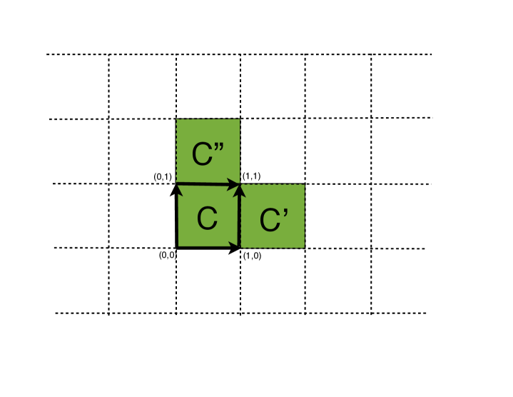
Figure 1. Consistency among cells $C,C^{\prime}$ and $C^{\prime\prime}$.

We rewrite (47) in the form

(52) $$\mathbf{Y}=\mathbf{\Phi}\mathbf{X}+{\mathbf{E}}.$$

subject to the constraint

(53) $$\Delta_{1}X_{2}=\Delta_{2}X_{1}$$

which is the discrete version of curl-free condition. This ensures that the reconstruction by line integration of $(v_{\mathbf{p}})$ from $\mathbf{X}$ is consistent (i.e. path-independent).

To see that (53) is necessary and sufficient for the recovery of $(v_{\mathbf{p}})$, consider, for example, the notations in Figure 1 and suppose $v_{0,0}$ is known. By definition of the difference operators $\Delta_{1},\Delta_{2}$ we have

$$v_{1,0} = v_{0,0}+(\Delta_{1}V)_{0,0}$$

$$v_{0,1} = v_{0,0}+(\Delta_{2}V)_{0,0}$$

In general, we can determine $v_{\mathbf{p}},\mathbf{p}\in\mathbb{L}$ iteratively from the relationship

$$v_{\mathbf{p}+\mathbf{e}_{1}} = v_{\mathbf{p}}+(\Delta_{1}V)_{\mathbf{p}}$$

$$v_{\mathbf{p}+\mathbf{e}_{2}} = v_{\mathbf{p}}+(\Delta_{2}V)_{\mathbf{p}}$$

and the knowledge of $V$ at any grid point. The path-independence in evaluating $v_{p_{1}+1,p_{2}+1}$

$$v_{p_{1}+1,p_{2}+1} =v_{p_{1},p_{2}}+(\Delta_{1}V)_{p_{1},p_{2}}+(\Delta_{2}V)_{p_{1}+1,p_{2}}$$

$$=v_{p_{1},p_{2}}+(\Delta_{2}V)_{p_{1},p_{2}}+(\Delta_{1}V)_{p_{1},p_{2}+1}$$

implies that

$$(\Delta_{2}V)_{p_{1}+1,p_{2}}-(\Delta_{2}V)_{p_{1},p_{2}}=(\Delta_{1}V)_{p_{1},p_{2}+1}-(\Delta_{1}V)_{p_{1},p_{2}}$$

which is equivalent to (53).

Now eq. (47) is equivalent to (52) with the constraint (53) provided that the value of $V$ at (any) one grid point is known. The equivalence between the original TV-min (48) and the CJS formulation (13) with $\mathbf{\Phi}_{j}=\mathbf{\Phi},\forall j$ then hinges on the equivalence of their respective feasible sets which can be established under the assumption of Gaussian noise. When $E$ in (47) is Gaussian noise, then so is ${\mathbf{E}}$ and vice versa, with variances precisely related to each other.

The random partial Fourier measurement matrix satisfies RIP with $n=\mathcal{O}(s)$, up to a logarithmic factor [3], while its mutual coherence $\mu$ behaves like $\mathcal{O}(n^{-1/2})$ [22]. Therefore (18) impies the sparsity constraint $s=\mathcal{O}(\sqrt{n})$ for the greedy approach which is more stringent than $s=\mathcal{O}(n)$ for the BPDN approach.

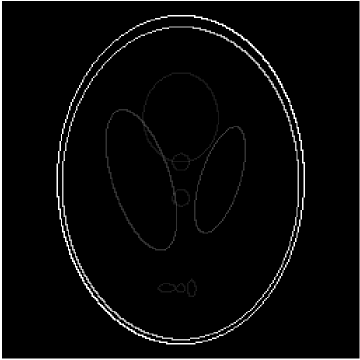
Figure 2. The original $256\times 256$ Shepp-Logan phantom (left), the Shepp-Logan phantom and the magnitudes of its gradient with sparsity $s=2184$.

7. Conclusion

We have developed a general CS theory (Theorems 1 and 2) for constrained joint sparsity with multiple sensing matrices and obtained performance guarantees parallel to those for the CS theory for single measurement vector and matrix.

From the general theory we have derived 2-norm error bounds for the object and the gradient, independent of the ambient dimension, for TV-min and greedy estimates of piecewise constant objects.

In addition, the CJS greedy algorithm can recover exactly the gradient support (i.e. the edges of the object) leading to an improved 2-norm error bound. Although the CJS greedy algorithm needs a higher number of measurement data than TV-min for Fourier measurements the incoherence property required is much easier to check and often the only practical way to verify RIP when the measurement matrix is not i.i.d. or Fourier.

We end by presenting a numerical example demonstrating the noise stability of the TV-min. Efficient algorithms for TV-min denoising/deblurring exist [1, 34]. We use the open source code L1-MAGIC (http://users.ece.gatech.edu/~justin/l1magic/) for our simulation.

Figure 2 shows the $256\times 256$ image of the Shepp-Logan Phantom (left) and the modulus of its gradient (right). Clearly the sparsity ($s=2184$) of the gradient is much smaller than that of the original image. We take $10000$ Fourier measurement data for the L1-min (1) and TV-min (5) reconstructions.

Figure 3. Noiseless L1-min reconstructed image (left) and the differences (middle) from the original image. The plot on the right is the gradient of the reconstructed image.

Because the image is not sparse, L1-min reconstruction produces a poor result even in the absence of noise, Figure 3. The relative error is $66.8\%$ in the $L2$ norm and $72.8\%$ in the TV norm. Only the outer boundary, which have the largest pixel values, is reasonably recovered.

Figure 4 shows the results of TV-min reconstruction in the presence of $5\%$ (top) or $10\%$ (bottom) noise. Evidently, the performance is greatly improved.

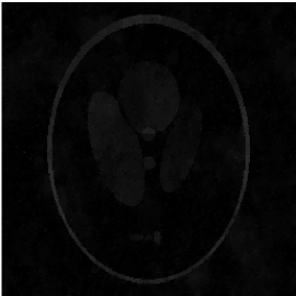
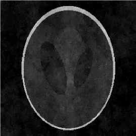
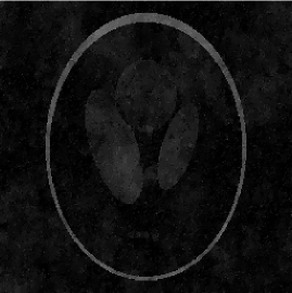
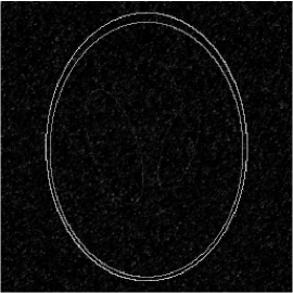
Figure 4. TV-reconstructed image with $5\%$ (top left) and $10\%$ (bottom left) and the respective differences (middle) from the original image. The plots on the right column are the magnitudes of the reconstructed image gradients.

Appendix A Proof of Theorem 1

The argument is patterned after [2] with adaptation to the CJS setting.

Proposition 1.

We have

$$\left|\Re\left\langle\varphi(\mathbf{Z}),\varphi(\mathbf{Z}^{\prime})\right\rangle\right|\leq\delta_{s+s^{\prime}}\|\mathbf{Z}\|_{2,2}\|\mathbf{Z}^{\prime}\|_{2,2}$$

for all $\mathbf{Z},\mathbf{Z}^{\prime}$ supported on disjoint subsets $T,T^{\prime}\subset\{1,...,m\}$ with $|S|\leq s,|S^{\prime}|\leq s^{\prime}.$

Proof.

Without loss of generality, suppose that $\|\mathbf{Z}\|_{2,2}=\|\mathbf{Z}^{\prime}\|_{2,2}=1$. Since $\mathbf{Z}\perp\mathbf{Z}^{\prime}$, $\|\mathbf{Z}\pm\mathbf{Z}^{\prime}\|^{2}_{2,2}=2.$ Hence we have from the RIP (14)

(54) $$2(1-\delta_{s+s^{\prime}})\leq\|\varphi(\mathbf{Z}\pm\mathbf{Z}^{\prime})\|_{2,2}^{2}\leq 2(1+\delta_{s+s^{\prime}})$$

By the parallelogram identity and (54)

$$\left|\Re\left\langle\varphi(\mathbf{Z}),\varphi(\mathbf{Z}^{\prime})\right\rangle\right|={1\over 4}\left|\|\varphi(\mathbf{Z})+\varphi(\mathbf{Z}^{\prime})\|_{2,2}^{2}-\|\varphi(\mathbf{Z})-\varphi(\mathbf{Z}^{\prime})\|_{2,2}^{2}\right|\leq\delta_{s+s^{\prime}}$$

which proves the proposition.

∎

By the triangle inequality and the fact that $\mathbf{X}$ is in the feasible set we have

(55) $$\|\varphi(\hat{\mathbf{X}}-\mathbf{X})\|_{2,2}\leq\|\varphi(\hat{\mathbf{X}})-\mathbf{Y}\|_{2,2}+\|\mathbf{Y}-\varphi(\mathbf{X})\|_{2,2}\leq 2\varepsilon.$$

Set $\hat{\mathbf{X}}=\mathbf{X}+\mathbf{D}$ and decompose $\mathbf{D}$ into a sum of $\mathbf{D}_{S_{0}},\mathbf{D}_{S_{1}},\mathbf{D}_{S_{2}},...,$ each of row-sparsity at most $s$. Here $S_{0}$ corresponds to the locations of the $s$ largest rows of $\mathbf{X}$; $S_{1}$ the locations of the $s$ largest rows of $\mathbf{D}_{S_{0}^{c}}$; $S_{2}$ the locations of the next $s$ largest rows of $\mathbf{D}_{S_{0}^{c}}$, and so on.

Step (i). Define the norm

$$\|\mathbf{Z}\|_{\infty,2}=\max_{j}\|\hbox{\rm row}_{j}(\mathbf{Z})\|_{2}.$$

For $j\geq 2$,

$$\|\mathbf{D}_{S_{j}}\|_{2,2}\leq s^{1/2}\|\mathbf{D}_{S_{j}}\|_{\infty,2}\leq s^{-1/2}\|\mathbf{D}_{S_{j-1}}\|_{2,2}$$

and hence

(56) $$\sum_{j\geq 2}\|\mathbf{D}_{S_{j}}\|_{2,2}\leq s^{-1/2}\sum_{j\geq 1}\|\mathbf{D}_{S_{j}}\|_{1,2}\leq s^{-1/2}\|\mathbf{D}_{S_{0}^{c}}\|_{1,2}.$$

This yields by the Cauchy-Schwarz inequality

(57) $$\|\mathbf{D}_{(S_{0}\cup S_{1})^{c}}\|_{2,2}=\|\sum_{j\geq 2}\mathbf{D}_{S_{j}}\|_{2,2}\leq\sum_{j\geq 2}\|\mathbf{D}_{S_{j}}\|_{2,2}\leq s^{-1/2}\|\mathbf{D}_{S_{0}^{c}}\|_{1,2}.$$

Also we have

$$\|\mathbf{X}\|_{1,2} \geq \|\hat{\mathbf{X}}\|_{1,2}$$

$$= \|\mathbf{X}_{S_{0}}+\mathbf{D}_{S_{0}}\|_{1,2}+\|\mathbf{X}_{S_{0}^{c}}+\mathbf{D}_{S_{0}^{c}}\|_{1,2}$$

$$\geq \|\mathbf{X}_{S_{0}}\|_{1,2}-\|\mathbf{D}_{S_{0}}\|_{1,2}-\|\mathbf{X}_{S_{0}^{c}}\|_{1,2}+\|\mathbf{D}_{S_{0}^{c}}\|_{1,2}$$

which implies

(58) $$\|\mathbf{D}_{S_{0}^{c}}\|_{1,2}\leq 2\|\mathbf{X}_{S_{0}^{c}}\|_{1,2}+\|\mathbf{D}_{S_{0}}\|_{1,2}.$$

Note that $\|\mathbf{X}_{S_{0}^{c}}\|_{1,2}=\|\mathbf{X}-\mathbf{X}^{(s)}\|_{1,2}$ by definition. Applying (57), (58) and the Cauchy-Schwartz inequality to $\|\mathbf{D}_{S_{0}}\|_{1,2}$ gives

(59) $$\|\mathbf{D}_{(S_{0}\cup S_{1})^{c}}\|_{2,2}\leq\|\mathbf{D}_{S_{0}}\|_{2,2}+2e_{0}$$

where $e_{0}\equiv s^{-1/2}\|\mathbf{X}-\mathbf{X}^{(s)}\|_{1,2}$.

Step (ii). Define the inner product

$$\left\langle{\mathbf{A}},{\mathbf{B}}\right\rangle=\sum_{i,j}A^{*}_{ij}B_{ij}$$

Observe

$$\|\varphi(\mathbf{D}_{S_{0}\cup S_{1}})\|_{2,2}^{2}$$

$$= \left\langle\varphi(\mathbf{D}_{S_{0}\cup S_{1}}),\varphi(\mathbf{D})\right\rangle-\left\langle\varphi(\mathbf{D}_{S_{0}\cup S_{1}}),\sum_{j\geq 2}\varphi(\mathbf{D}_{S_{j}})\right\rangle$$

$$= \Re\left\langle\varphi(\mathbf{D}_{S_{0}\cup S_{1}}),\varphi(\mathbf{D})\right\rangle-\sum_{j\geq 2}\Re\left\langle\varphi(\mathbf{D}_{S_{0}\cup S_{1}}),\varphi(\mathbf{D}_{S_{j}})\right\rangle$$

$$= \Re\left\langle\varphi(\mathbf{D}_{S_{0}\cup S_{1}}),\varphi(\mathbf{D})\right\rangle-\sum_{j\geq 2}\left[\Re\left\langle\varphi(\mathbf{D}_{S_{0}}),\varphi(\mathbf{D}_{S_{j}})\right\rangle+\Re\left\langle\varphi(\mathbf{D}_{S_{1}}),\varphi(\mathbf{D}_{S_{j}})\right\rangle\right].$$

From (55) and the RIP (14) it follows that

$$|\left\langle\varphi(\mathbf{D}_{S_{0}\cup S_{1}}),\varphi(\mathbf{D})\right\rangle| \leq\|\varphi(\mathbf{D}_{S_{0}\cup S_{1}})\|_{2,2}\|\varphi(\mathbf{D})\|_{2,2} \leq 2\varepsilon\sqrt{1+\delta_{2s}}\|\mathbf{D}_{S_{0}\cup S_{1}}\|_{2,2}.$$

Moreover, it follows from Proposition 1 that

(61) $$\left|\Re\left\langle\varphi(\mathbf{D}_{S_{0}}),\varphi(\mathbf{D}_{S_{j}})\right\rangle\right| \leq \delta_{2s}\|\mathbf{D}_{S_{0}}\|_{2,2}\|\mathbf{D}_{S_{j}}\|_{2,2}$$

(62) $$\left|\Re\left\langle\varphi(\mathbf{D}_{S_{1}}),\varphi(\mathbf{D}_{S_{j}})\right\rangle\right| \leq \delta_{2s}\|\mathbf{D}_{S_{0}}\|_{2,2}\|\mathbf{D}_{S_{j}}\|_{2,2}$$

for $j\geq 2$. Since $S_{0}$ and $S_{1}$ are disjoint

$$\|\mathbf{D}_{S_{0}}\|_{2,2}+\|\mathbf{D}_{S_{1}}\|_{2,2}\leq\sqrt{2}\sqrt{\|\mathbf{D}_{S_{0}}\|^{2}_{2,2}+\|\mathbf{D}_{S_{1}}\|^{2}_{2,2}}=\sqrt{2}\|\mathbf{D}_{S_{0}\cup S_{1}}\|_{2,2}.$$

Also by (A)-(62) and RIP

$$(1-\delta_{2s})\|\mathbf{D}_{S_{0}\cup S_{1}}\|_{2,2}^{2}\leq\|\varphi(\mathbf{D}_{S_{0}\cup S_{1}})\|_{2,2}^{2}\leq\|\mathbf{D}_{S_{0}\cup S_{1}}\|_{2,2}\left(2\varepsilon\sqrt{1+\delta_{2s}}+\delta_{2s}\sum_{j\geq 2}\|\mathbf{D}_{S_{j}}\|_{2,2}\right).$$

Therefore from (56) we obtain

$$\|\mathbf{D}_{S_{0}\cup S_{1}}\|_{2,2}\leq\alpha\varepsilon+\rho s^{-1/2}\|\mathbf{D}_{S_{0}^{c}}\|_{1,2},\quad\alpha={2\sqrt{1+\delta_{2s}}\over 1-\delta_{2s}},\quad\rho={{\sqrt{2}}\delta_{2s}\over 1-\delta_{2s}}$$

and moreover by (58) and the definition of $e_{0}$

$$\|\mathbf{D}_{S_{0}\cup S_{1}}\|_{2,2}\leq\alpha\varepsilon+\rho\|\mathbf{D}_{S_{0}}\|_{2,2}+2\rho e_{0}$$

after applying the Cauchy-Schwartz inequality to bound $\|\mathbf{D}_{S_{0}}\|_{1,2}$ by $s^{1/2}\|\mathbf{D}_{S_{0}}\|_{2,2}$. Thus

$$\|\mathbf{D}_{S_{0}\cup S_{1}}\|_{2,2}\leq(1-\rho)^{-1}(\alpha\varepsilon+2\rho e_{0})$$

if (14) holds.

Finally,

$$\|\mathbf{D}\|_{2,2} \leq \|\mathbf{D}_{S_{0}\cup S_{1}}\|_{2,2}+\|\mathbf{D}_{(S_{0}\cup S_{1})^{c}}\|_{2,2}$$

$$\leq 2\|\mathbf{D}_{S_{0}\cup S_{1}}\|_{2,2}+2e_{0}$$

$$\leq 2(1-\rho)^{-1}(\alpha\varepsilon+(1+\rho)e_{0})$$

which is the desired result.

Appendix B Proof of Theorem 2

We prove the theorem by induction.

Let $\hbox{supp}(\mathbf{X})={\mathcal{S}}=\{J_{1},\ldots,J_{s}\}$ and

$$X_{\rm max}=\|\hbox{\rm row}_{J_{1}}(\mathbf{X})\|_{1}\geq\|\hbox{row}_{J_{2}}(\mathbf{X})\|_{1}\geq\cdots\geq\|\hbox{\rm row}_{J_{s}}(\mathbf{X})\|_{1}=X_{\rm min}$$

. In the first step,

$$\sum_{j=1}^{d}|\Phi^{*}_{j,J_{1}}Y_{j}| = \sum_{j=1}^{d}|{X}_{J_{1}j}+X_{J_{2}j}\Phi_{j,J_{1}}^{*}\Phi_{j,J_{2}}+...+X_{J_{s}j}\Phi_{j,J_{1}}^{*}\Phi_{j,J_{s}}+\Phi^{*}_{j,J_{1}}E_{j}|$$

$$\geq X_{\rm max}-X_{\rm max}(s-1)\mu_{\rm max}-\sum_{j}\|E_{j}\|_{2}.$$

On the other hand, $\forall l\notin\hbox{supp}(\mathbf{X})$,

$$\sum_{j=1}^{d}|\Phi_{j,l}^{*}Y_{j}| = \sum_{j=1}^{d}|X_{J_{1}j}\Phi^{*}_{j,l}\Phi_{j,J_{1}}+X_{J_{2}j}\Phi_{j,l}^{*}\Phi_{j,J_{2}}+...+X_{J_{s}j}\Phi_{j,l}^{*}\Phi_{j,J_{s}}+\Phi_{j,l}^{*}E_{j}|$$

$$\leq X_{\rm max}s\mu_{\rm max}+\sum_{j}\|E_{j}\|_{2}.$$

Hence, if

$$(2s-1)\mu_{\rm max}+\frac{2\sum_{j}\|E_{j}\|_{2}}{X_{\rm max}}<1,$$

then the right hand side of (B) is greater than the right hand side of (B) which implies that the first index selected by OMP must belong to $\hbox{supp}(\mathbf{X})$.

To continue the induction process, we state the straightforward generalization of a standard uniqueness result for sparse recovery to the joint sparsity setting (Lemma 5.3, [19]).

Proposition 2.

Let $\mathbf{Z}=\varphi(\mathbf{X})$ and $\mathbf{Y}=\mathbf{Z}+{\mathbf{E}}$. Let ${\mathcal{S}}^{k}$ be a set of $k$ indices and let $\mathbf{A}\in\mathbb{C}^{n\times d}$ with ${\hbox{supp}}{(\mathbf{A})}={\mathcal{S}}^{k}$. Define

(65) $$\mathbf{Y}^{\prime}=\mathbf{Y}-\varphi(\mathbf{A})$$

and

$$\mathbf{Z}^{\prime}=\mathbf{Z}-\varphi(\mathbf{A}).$$

Clearly, $\mathbf{Y}^{\prime}=\mathbf{Z}^{\prime}+{\mathbf{E}}$. If ${\mathcal{S}}^{k}\subsetneq\hbox{supp}(\mathbf{X})$ and the sparsity $s$ of $\mathbf{X}$ satisfies $2s<1+\mu_{\rm max}^{-1}$, then $\mathbf{Z}^{\prime}$ has a unique sparsest representation $\mathbf{Z}^{\prime}=\varphi(\mathbf{X}^{\prime})$ with the sparsity of $\mathbf{X}^{\prime}$ at most $s$.

Proposition 2 says that selection of a column, followed by the formation of the residual signal, leads to a situation like before, where the ideal noiseless signal has no more representing columns than before, and the noise level is the same.

Suppose that the set ${\mathcal{S}}^{k}\subseteq{\hbox{supp}}(\mathbf{X})$ of $k$ distinct indices has been selected and that $\mathbf{A}$ in Proposition 2 solves the following least squares problem

(66) $$\mathbf{A}=\hbox{arg}\min\|\mathbf{Y}-\mathbf{\Phi}\mathbf{B}\|_{2,2},\quad\hbox{s.t.}\quad{\hbox{supp}}(\mathbf{B})\subseteq{\mathcal{S}}^{k}$$

without imposing the constraint ${\mathcal{L}}$. This is equivalent to the concatenation $\mathbf{A}=[A_{j}]$ of $d$ separate least squares solutions

(67) $${A}_{j}=\hbox{arg}\min_{B_{j}}\|Y_{j}-\mathbf{\Phi}_{j}B_{j}\|_{2},\quad\hbox{s.t.}\quad{\hbox{supp}}(B_{j})\subseteq{\mathcal{S}}^{k}$$

Let $\mathbf{\Phi}_{j,{\mathcal{S}}^{k}}$ be the column submatrix of $\mathbf{\Phi}_{j}$ indexed by the set ${\mathcal{S}}^{k}$. By (65) and (67), $\mathbf{\Phi}^{*}_{j,{\mathcal{S}}^{k}}Y^{\prime}_{j}=0,\forall j,$ which implies that no element of ${\mathcal{S}}^{k}$ gets selected at the $(k+1)$-st step.

In order to ensure that some element in ${\hbox{supp}}(\mathbf{X})\setminus{\mathcal{S}}^{k}$ gets selected at the $(k+1)$-st step we only need to repeat the calculation (B)-(B) to obtain the condition

(68) $$(2s-1)\mu_{\rm max}+\frac{2\sum_{j}\|E_{j}\|_{2}}{\|X_{J_{k+1}}\|_{1}}<1.$$

Since $\sum_{j}\|E_{j}\|_{2}\leq\sqrt{d}\|{\mathbf{E}}\|_{2,2}=\sqrt{d}\varepsilon$ (68) follows from

(69) $$(2s-1)\mu_{\rm max}+\frac{2\sqrt{d}\varepsilon}{X_{\rm min}}<1$$

which is the same as (18) and allows us to apply Proposition 2 repeatedly.

By the $s$-th step, all elements of the support set are selected and by the nature of the least squares solution the $2$-norm of the residual is at most $\varepsilon$. Thus the stopping criterion is met and the iteration stops after $s$ steps.

On the other hand, it follows from the calculation

$$\sum_{j}\|Y^{\prime}_{j}\|_{2} \geq \sum^{d}_{j=1}\big{|}\Phi^{*}_{j,J_{k+1}}Y^{\prime}_{j}\big{|}$$

$$= \sum_{j}\big{|}X_{J_{k+1}j}+\sum_{i=k+2}^{s}X_{J_{i}i}\Phi_{j,J_{k+1}}^{*}\Phi_{i,J_{i}}+\Phi_{j,J_{k+1}}^{*}E_{j}\big{|}$$

$$\geq \|\hbox{\rm row}_{J_{k+1}}(\mathbf{X})\|_{1}-\mu_{\rm max}(s-k-1)\|\hbox{\rm row}_{J_{k+2}}(\mathbf{X})\|_{1}-\sum_{j}\|E_{j}\|_{2}$$

$$\geq (1-\mu_{\rm max}(s-k-1))\|\hbox{\rm row}_{J_{k+1}}(\mathbf{X})\|_{1}-\sum_{j}\|E_{j}\|_{2}$$

and (69) (equivalently, $X_{\rm min}(1-\mu_{\rm max}(2s-1))>2\sqrt{d}\varepsilon$) that $\|\mathbf{Y}\|_{1,2}>\sqrt{d}\varepsilon$ for $k=0,1,\cdots,s-1$. Thus the iteration does not stop until $k=s$.

Since $\hat{\mathbf{X}}$ be the solution of the least squares problem (19), we have

$$\|\mathbf{Y}-\mathbf{\Phi}\hat{\mathbf{X}}\|_{2,2}\leq\|\mathbf{Y}-\mathbf{\Phi}\mathbf{X}\|_{2,2}\leq\varepsilon$$

and

$$\|\mathbf{\Phi}(\mathbf{X}-\hat{\mathbf{X}})\|^{2}_{2,2}\leq 2\|\mathbf{Y}-\mathbf{\Phi}\mathbf{X}\|^{2}_{2,2}+2\|\mathbf{Y}-\mathbf{\Phi}\hat{\mathbf{X}}\|^{2}_{2,2}\leq 2\varepsilon^{2}$$

which implies

$$\|\hat{\mathbf{X}}-\mathbf{X}\|_{2,2}\leq\sqrt{2}\varepsilon/\lambda_{\rm min}$$

where

$$\lambda_{\rm min}=\min_{j}\{\hbox{\rm the $s$-th singular value of the column submatrix of $\mathbf{\Phi}_{j}$ indexed by ${\mathcal{S}}$}\}$$

.

The desired error bound (20) can now be obtained from the following result (Lemma 2.2, [19]).

Proposition 3.

Suppose $s<1+\mu(\mathbf{\Phi}_{j})^{-1}$. Every $m\times s$ column submatrix of $\mathbf{\Phi}_{j}$ has the $s$-th singular value bounded below by $\sqrt{1-\mu(\mathbf{\Phi}_{j})(s-1)}$.

By Proposition 3, $\lambda_{\rm min}\geq\sqrt{1-\mu_{\rm max}(s-1)}$ and thus

$$\|\hat{\mathbf{X}}-\mathbf{X}\|_{2,2}\leq{\sqrt{2}\varepsilon\over\sqrt{1-\mu_{\rm max}(s-1)}}.$$

Acknowledgement. I thank Stan Osher and Justin Romberg for suggestion of publishing this note at the IPAM workshop “Challenges in Synthetic Aperture Radar” February 6-10, 2012. I thank the anonymous referees and Deanna Needell for pointing out the reference [25] which helps me appreciate more deeply the strength and weakness of my approach. I am grateful to Wenjing Liao for preparing Fig. 2-4. The research is partially supported by the U.S. National Science Foundation under grant DMS - 0908535.

References

[1]
A. Beck and M. Teboulle,
”Fast gradient-based algorithms for constrained total variation image denoising and deblurring Problems”,
IEEE Trans. Image Proc.18 (11), 2419-2434, 2009.
[2]
E. J. Candès, “The restricted isometry property and its implications for compressed sensing,” Compte Rendus de l’Academie des Sciences, Paris, Serie I.346 (2008) 589-592.
[3]
E. J. Candès, J. Romberg and T. Tao, “Robust uncertainty principle: exact signal reconstruction from highly incomplete frequency information,” IEEE Trans. Inform. Theory52 (2006), 489 – 509.
[4]
E.J. Candès and Y. Plan, “Near-ideal model selection
by minimization,” Ann. Stat.37 (2009), 2145-2177.
[5]
E. J. Candès and T. Tao, “ Decoding by linear programming,” IEEE Trans. Inform. Theory51 (2005), 4203 – 4215.
[6]
A. Chambolle, “An algorithm for total variation minimization
and applications,” J. Math. Imaging Vision20
(2004), 89-97.
[7]
A. Chambolle and P.-L. Lions, ”Image recovery via total variation minimization
and related problems, ” Numer. Math.76 (1997), 167-188.
[8]
T. F. Chan, G. H. Golub, and P. Mulet, A nonlinear primal-dual method for total variation-based image restoration., SIAM J. Sci. Comput.20 (6), pp. 1964 1977, 1999,
[9]
T. Chan and J. Shen, Image Processing And Analysis: Variational, PDE, Wavelet and Stochastic Methods, Society for Industrial and Applied Mathematics, 2005.
[10]
J. Chen and X. Huo, “Theoretical results on sparse representations of mulitple-measurement vectors,” IEEE Trans. Signal Proc.54 (2006), 4634-4643.
[11]
S.S. Chen, D.L. Donoho and M.A. Saunders,
“Atomic decomposition by basis pursuit,” SIAM Rev.43 (2001), 129-159.
[13] J. F. Claerbout and F. Muir “Robust modeling with erratic data,” Geophysics38 (1973), no. 5, 826-844.
[14]
D. Colton and R. Kress, Inverse Acoustic and Electromagnetic Scattering Theory. 2nd edition, Springer, 1998.
[15]
S.F. Cotter, B.D. Rao, K. Engan and K. Kreutz-Delgado, “Sparse solutions to linear
inverse problems with multiple measurement vectors,”
IEEE Trans. Signal Proc.53 (2005), 2477- 2488.
[16]
G.M. Davis, S. Mallat and M. Avellaneda, “Adaptive greedy approximations”, J. Constructive Approx. 13 (1973), 57-98.
[17]
D. L. Donoho, “Compressed sensing,” IEEE Trans. Inform. Theory52 (2006) 1289 – 1306.
[18]
D.L. Donoho and M. Elad, “Optimally
sparse representation in general (nonorthogonal)
dictionaries via minimization,”
Proc. Nat. Acad. Sci. 100 (2003), 2197-2202.
[19]
D.L. Donoho, M. Elad and V.N. Temlyakov,
“Stable recovery of sparse overcomplete
representations in the presence of noise,”
IEEE Trans. Inform. Theory52 (2006) 6-18.
[20]
D.L. Donoho and X. Huo, “Uncertainty principle
and ideal atomic decomposition, ” IEEE Trans. Inform. Theory47 (2001), 2845-2862.
[21]
A. Fannjiang, “ Compressive inverse scattering II. Multi-shot SISO measurements with Born scatterers,”
Inverse Problems26 (2010), 035009
[22]
A. Fannjiang, T. Strohmer and P. Yan, “Compressed Remote Sensing of Sparse Object,” SIAM J. Imag.
Sci.3 (2010) 596-618.
[23]
G.H. Golub and C.F. Van Loan, Matrix Computations, 3rd edition.
The Johns Hopkins University Press, 1996.
[24]
F. Natterer, The Mathematics of Computerized Tomography,
John Wiley & Sons, 1986.
[25]
D. Needell and R. Ward, “Stable image reconstruction using total variation minimization,” arXiv:1202.6429v6, May 31, 2012.
[26]
V. Patel, R Maleh, A. Gilbert, and R. Chellappa, “ Gradient-based image recovery methods from incomplete Fourier measurements,” IEEE Trans. Image Process.21 (2012), 94-104.
[27]
Y.C. Pati, R. Rezaiifar and P.S. Krishnaprasad, “Orthogonal
matching pursuit: recursive function approximation with applications
to wavelet decomposition,” Proceedings of the 27th Asilomar Conference in Signals, Systems and Computers, 1993.
[28]
J. Romberg, “Imaging via compressive sampling,” IEEE Sign. Proc. Mag.20, 14-20, 2008.
[29]
L. Rudin and S. Osher, “Total variation based image restoration with free local constraints,” Proc. IEEE ICIP1 (1994), pp. 31 35.
[30]
L.I. Rudin, S. Osher and E. Fatemi, ” Nonlinear total
variation based noise removal algorithms,” Physica D60 (1992) 259-268.
[31] H. L. Taylor, S. C. Banks, J. F. McCoy, “Deconvolution with the -1 norm,” Geophysics44 (1979), no. 1, 39-52.
[32]
J.A. Tropp, “Greed is good: algorithmic results for sparse approximation,” IEEE Trans. Inform. Theory50 (2004), 2231-2242.
[33] J. A. Tropp, A. C. Gilbert, and M. J. Strauss, Algorithms for simultaneous sparse approximation. Part I: Greedy pursuit, Signal Process. (Special Issue on Sparse Approximations in Signal and Image Processing) 86 (2006), 572-588.
[34]
P. Weiss, L. Blanc-Féraud and G. Aubert,
“Efficient schemes for total variation minimization under constraints in image processing,”
SIAM J. Sci. Comput31 (3), pp. 2047 2080, 2009.