Symmetric and asymmetric solitons in a nonlocal nonlinear coupler

Abstract

We study effects of nonlocality of the cubic self-focusing nonlinearity on the stability and symmetry-breaking bifurcation (SBB) of solitons in the model of a planar dual-core optical waveguide with nonlocal (thermal) nonlinearity. In comparison with the well-known coupled systems with the local nonlinearity, the present setting is affected by the competition of different spatial scales, viz., the coupling length and correlation radius of the nonlocality, $\sqrt{d}$. By means of numerical methods and variational approximation (VA, which is relevant for small $d$), we find that, with the increase of the correlation radius, the SBB changes from subcritical into supercritical, which makes all the asymmetric solitons stable. On the other hand, the nonlocality has little influence on the stability of antisymmetric solitons. Analytical results for the SBB are also obtained (actually, for antisymmetric “accessible solitons”) in the opposite limit of the ultra-nonlocal nonlinearity, using a coupler based on the Snyder-Mitchell model. The results help to grasp the general picture of the symmetry breaking in nonlocal couplers.

I Introduction

Dual-core systems, featuring intrinsic nonlinearity in parallel cores coupled by linear tunneling of wave fields, find their realizations in various physical settings. Well-known systems of this type in optics are twin-core fibers twin -Snyder (see also an early review Wabnitz ) and Bragg gratings Mak , as well as double planar waveguides with the second-harmonic-generating intrinsic nonlinearity Mak-chi2 . Similar settings for matter waves are represented by two-layer Bose-Einstein condensates Arik -Santos . A fundamental physical effect in nonlinear symmetric dual-core systems is the symmetry-breaking bifurcation (SBB), alias the phase transition, which destabilizes symmetric modes and gives rise to asymmetric ones. In nonlinear optics, the SBB was studied in detail for continuous-wave (spatially uniform) states Snyder and solitons dual-core ; Mak in twin-core fibers exact ; Laval , Maim -1996 and Bragg gratings Mak with the Kerr (cubic) nonlinearity, as well as for solitons in double-core waveguides with the quadratic Mak-chi2 and cubic-quintic Lior nonlinearity. The SBB was studied too for matter-wave solitons in two-layer BEC settings Arik ; Warsaw .

The self-focusing cubic nonlinearity gives rise to the SBB of the subcritical type (alias the phase transition of the first kind) for solitons in the symmetric dual-core system. The bifurcation of this type is characterized by originally unstable branches of emerging asymmetric modes, which at first extend backward (in the direction of weaker nonlinearity), and then turn forward, retrieving the stability at the turning points bifurcations . In this case, the system demonstrates a bistability and hysteresis in a limited interval, characteristic to phase transitions of the first kind. If the dual-core system is equipped with a periodic potential (lattice) acting in the direction transversal to the propagation coordinate, the character of the SBB changes to supercritical above a certain threshold value of the lattice’s strength Warsaw . The supercritical bifurcation (alias the phase transition of the second kind) gives rise to stable branches of asymmetric modes going in the forward direction bifurcations . The SBBs belong to this type too in the twin-core Bragg grating, and in quadratically nonlinear waveguides Mak ; Mak-chi2 .

In addition to numerical analysis of symmetric, antisymmetric and asymmetric soliton modes in dual-core system with the intrinsic cubic nonlinearity dual-core ; anti , the bifurcation point was found in an exact analytical form exact , and the emerging asymmetric solitons were studied in detail by means of the variational approximation (VA) Laval ; Maim ; Pak ; 1996 . The latter method is relevant for studies of solitons in many models originating in nonlinear optics and related fields VA , while the possibility to find the exact bifurcation point is a feature specific to particular systems.

The nonlinear response in optical media may feature spatial nonlocality, which means that the local change of the refractive index induced by the light beam depends on the distribution of the light intensity in a vicinity of a given point ScienceNonlocal ; ReviewNonlocal . The nonlocality arises when the nonlinear optical response involves mechanisms such as heat diffusion, as analyzed theoretically Krolik and demonstrated experimentally MotiPRL ; Canberra , molecular reorientation in liquid crystals AssantoPRL1 ; AssantoPRL2 , atomic diffusion SuterPRA ; KrolikPRL ; YePRA , etc. The fields of nanophotonics and plasmonics also give rise to effective nonlocalities, due to light-matter interactions occurring in these media on deeply subwavelength scales nano ; Romania .

Nonlocal nonlinearities are known in other physical media, including plasmas plasma and self-gravitating photonic beams Rivlin . Long-range interactions play an important role in dipolar Bose-Einstein condensates (BECs) too DD , and nonlocal gravity-like interactions can be induced in BEC by means of laser illumination quasi-gravity .

The nonlocality, which introduces a new spatial scale, namely, the correlation radius (denoted below as $\sqrt{d}$), may drastically alter nonlinear excitations in optical systems, due to the interplay of $\sqrt{d}$with other natural scales. In particular, the nonlocality changes the character of interactions between solitons AssantoOL , and it suppresses the beam’s collapse and transverse instabilities KonotopPRE ; OBangPRE . The nonlocality also accounts for the formation of new types of soliton modes YeOLTwin ; YeOLBending . However, to the best of knowledge, the influence of nonlocality on the performance of optical couplers has not been reported yet. In particular, new effects may be expected due to the competition of $\sqrt{d}$ with the coupling length, i.e., the interplay of nonlocal and local interactions. This is the objective of the present work.

We consider the formation of solitons in a planar dual-core waveguide, in which the nonlocal nonlinearity of the thermal type acts in both cores, while the coupling between them remains linear and local, as the heat diffusion does  not transfer energy across the gap separating the waveguides. Similar to couplers with the local nonlinearity, the nonlocal model gives rise to three types of solitons, viz., symmetric, antisymmetric and asymmetric ones. However, the nonlocality significantly affects the symmetry-breaking phase transition (SBB) for solitons, as well as stability of the emerging asymmetric solitons, which are basic properties of nonlinear couplers: at a critical value of the $\sqrt{d}$, the SBB changes its character from sub- to supercritical. Taking into regard the potential that nonlinear couplers have for various application to photonics, such as all-optical switching switch ; Wabnitz , the use of the nonlocality for the control of the soliton dynamics in these systems may help to expand the range of the applications. While our analysis is performed in terms of the thermal nonlinearity in optical waveguides, the results may plausibly apply to other dual-core physical systems which feature the nonlocal nonlinearity.

The paper is organized as follows. The model is formulated in Section II, and analytical results are reported in Section III. These results are obtained by means of the VA for solitons in the case of weak nonlocality (small $\sqrt{d}$), and, on the other hand, the SBB is also investigated (in fact, for antisymmetric solitons) in the opposite limit of the ultra-nonlocal nonlinearity, in terms of a coupled system for “accessible solitons” [the Snyder-Mitchell (SM) model ScienceNonlocal ]. In particular, the exact bifurcation point is found for the SM system. The results for the small correlation radius explicitly demonstrate the shift of the SBB point to larger values of the soliton’s power, and the trend to the transition of the subcritical bifurcation into the supercritical one, while the findings reported for the ultra-nonlocal system help to apprehend the general situation. Numerical results, which provide the full description of solitons in the nonlocal dual-core system for moderate values of the correlation radius, are presented in Section IV. In the case of the weak nonlocality, these results verify the analytical results produced by the VA. The paper is concluded by Section V.

II The model

The propagation of optical beams along axis $z$ in the planar dual-core waveguide with the intrinsic self-focusing nonlinearity of the thermal type Krolik ; ReviewNonlocal is described by the system of linearly coupled nonlinear Schrödinger (NLS) equations for complex field amplitudes $u$, $v$ in the two cores, and respective local perturbations $m,n$ of the refractive index:

$$iu_{z}+\frac{1}{2}u_{xx}+mu+v=0,$$ (1a)

$$iv_{z}+\frac{1}{2}v_{xx}+nv+u=0,$$ (1b)

$$m-dm_{xx}=|u|^{2},$$ (1c)

$$n-dn_{xx}=|v|^{2},$$ (1d)

where $$x v u 1 \sim 1 d d$$ is the transverse coordinate, the coupling constant [the coefficient in front of terms and in Eqs. (1a) and (1b), respectively] is scaled to be (accordingly, the coupling length is also ), and is the squared correlation radius of the nonlocality. In fact, controls the competition between the length scales determined by the nonlocal and local interactions in the system.

Stationary solutions to Eqs. (1) with propagation constant $b$ are looked for as

$$u\left(z,x\right)=e^{ibz}U(x),v\left(z,x\right)=e^{ibz}V(x),$$ (2a)

$$m=m(x),n=n(x),$$ (2b)

with real functions $$U(x) V(x)$$ and obeying the following equations:

$$-bU+\frac{1}{2}U^{\prime\prime}+mU+V=0,$$ (3a)

$$-bV+\frac{1}{2}V^{\prime\prime}+nV+U=0,$$ (3b)

$$m-dm^{\prime\prime}=U^{2},$$ (3c)

$$n-dn^{\prime\prime}=V^{2}.$$ (3d)

Equations (1) conserve the total power,

$$P=P_{u}+P_{v}\equiv\int_{-\infty}^{\infty}|u|^{2}dx+\int_{-\infty}^{\infty}|v|^{2}dx.$$ (4)

Obviously, symmetric [$U(x)=V(x)$] and antisymmetric $[U(x)=-V(x)]$ modes have $P_{1}=P_{2}$, while asymmetric ones can be characterized by parameter

$$\Theta=\frac{P_{2}-P_{1}}{P_{2}+P_{1}},$$ (5)

which takes values $-1<\Theta<+1$.

Parallel to Eqs. (1), it is relevant to consider the ultra-nonlocal model, taken in the form of two linearly coupled SM equations ScienceNonlocal ,

$$iu_{z}+\frac{1}{2}u_{xx}-\frac{1}{2}P_{u}x^{2}u+v=0,$$ (6a)

$$iv_{z}+\frac{1}{2}v_{xx}-\frac{1}{2}P_{v}x^{2}v+u=0,$$ (6b)

where $$P_{1,2}$$ are the powers defined as per Eq. (4). Actually, Eqs. (6) correspond to the version of Eqs. (1c) and (1d) with spatially averaged right-hand sides. To the best of our knowledge, the SM coupler was not considered before, while the extreme nonlocality postulated in the SM model per se finds realizations and applications in diverse optical SM-optical and optomechanical SM-optomech settings.

III Analytical results

III.1 The variational approximation for the weakly nonlocal system

To apply the VA to the present system, we note that, in the case of weak nonlocality ($d\ll 1$), Eqs. (3c) and (3d) yield, in the first approximation, $m=U^{2}+d\left(U^{2}\right)^{\prime\prime}$, and $n=V^{2}+d\left(V^{2}\right)^{\prime\prime}$ Krol . The substitution of this approximation into Eqs. (3a) and (3b) leads to a system of two coupled equations with nonlinear-diffraction terms:

$$-bU+\frac{1}{2}U^{\prime\prime}+U^{3}+dU\left(U^{2}\right)^{\prime\prime}+V=0,$$ (7a)

$$-bV+\frac{1}{2}V^{\prime\prime}+V^{3}+dV\left(V^{2}\right)^{\prime\prime}+U=0,$$ (7b)

which may be derived from the Lagrangian with density

$$\mathcal{L} = \frac{1}{4}\left[\left(U^{\prime}\right)^{2}+\left(V^{\prime}\right)^{2}\right]+\frac{b}{2}\left(U^{2}+V^{2}\right)-\frac{1}{4}\left(U^{4}+V^{4}\right)$$ (8)

$$+d\left[U^{2}\left(U^{\prime}\right)^{2}+V^{2}\left(V^{\prime}\right)^{2}\right]-UV.$$

The ansatz for soliton solutions may be naturally chosen as

$$\left\{U(x),V(x)\right\}=\left\{A,B\right\}\mathrm{sech}\left(x/W\right),$$ (9)

where $A$ and $B$ are amplitudes of the two components, and $W$ is their common width. The substitution of the ansatz into density (8) and evaluation of the integrals yields the corresponding Lagrangian,

$$L\equiv\int_{-\infty}^{+\infty}\mathcal{L}dx=\frac{A^{2}+B^{2}}{6W}+b\left(A^{2}+B^{2}\right)W$$

$$-\frac{1}{3}\left(A^{4}+B^{4}\right)W+\frac{4d\left(A^{4}+B^{4}\right)}{15W}-2ABW.$$ (10)

This Lagrangian can be more conveniently rewritten in terms of the total power $P$, see Eq. (4), and power imbalance $Q=P_{1}-P_{2}$,

$$2\left(A^{2}+B^{2}\right)W\equiv P,~{}2\left(A^{2}-B^{2}\right)W\equiv Q,$$ (11)

as follows:

$$2L=\frac{P}{6W^{2}}+bP-\frac{P^{2}+Q^{2}}{12W}$$ (12)

$$+\frac{d}{15}\frac{P^{2}+Q^{2}}{W^{3}}-\sigma\sqrt{P^{2}-Q^{2}},$$ (13)

where $\sigma=1$ for symmetric solitons and asymmetric ones generated from them by the SBB, and $\sigma=-1$ for antisymmetric solitons. The corresponding Euler-Lagrange equations are $\partial L/\partial W=\partial L/\partial Q=\partial L/\partial P=0$, i.e.,

$$-\frac{P}{W}+\frac{P^{2}+Q^{2}}{4}-\frac{3d}{5}\frac{P^{2}+Q^{2}}{W^{2}}=0,$$ (14)

$$Q\left(-\frac{1}{6W}+\frac{2d}{15W^{3}}+\frac{\sigma}{\sqrt{P^{2}-Q^{2}}}\right)=0,$$ (15)

$$b=\frac{P}{6W}-\frac{1}{6W^{2}}-\frac{2dP}{15W^{3}}+\frac{\sigma P}{\sqrt{P^{2}-Q^{2}}}$$ (16)

Equation (16), which determines the propagation constant, $b$, is detached from Eqs. (14) and (15). Equation (15) yields either $Q=0$, which corresponds to symmetric and antisymmetric solitons, or

$$-\frac{1}{6W}+\frac{2d}{15W^{3}}+\frac{1}{\sqrt{P^{2}-Q^{2}}}=0$$ (17)

for asymmetric ones. Further, the expansion of Eqs. (14) and (16) for small $d$, i.e., the weak nonlocality, yields

$$W\approx\frac{4}{P}+\frac{3d}{5}P,~{}b\approx\frac{1}{32}P^{2}+\sigma-\frac{d}{192}P^{4},$$ (18)

which predicts that, naturally, the nonlocality makes the soliton wider, for given total power $P$. This is confirmed by the numerical solutions, as shown below.

The most essential point is to find the critical power $P_{\mathrm{bif}}$, at which the asymmetric solitons bifurcate from the symmetric ones. This value is determined by a system of equations (14) and (17), in which one should set $Q=0$. Further, using the assumption of the weak nonlocality, i.e., small $d$, the ensuing solution for $P_{\mathrm{bif}}$ can be expanded up to order $d$, which yields

$$P_{\mathrm{bif}}=2\sqrt{6}+\left(24\sqrt{6}/5\right)d.$$ (19)

Note that, at $d=0$, Eq. (19) gives $P_{\mathrm{bif}}(d=0)=2\sqrt{6}$ 1996 , which may be compared to the known exact result exact , $\left(P_{\mathrm{bif}}\right)_{\mathrm{exact}}=8/\sqrt{3}$, the relative error being $0.0\allowbreak 57$.

The VA predicts, as per Eq. (19), the increase of the soliton’s power at the bifurcation point due to the weak nonlocality. To compare the prediction with the numerical findings, we take the slope of the $P_{\mathrm{bif}}(d)$ dependence at $d=0$, for which Eq. (19) yields

$$\left[\frac{d(P_{\mathrm{bif}})}{d(d)}|_{d=0}\right]_{\mathrm{variational}}=24\sqrt{6}/5\approx\allowbreak 11.758.$$ (20)

On the other hand, the same slope obtained from the numerical solution (see the next section) is

$$\left[\frac{d(P_{\mathrm{bif}})}{d(d)}|_{d=0}\right]_{\mathrm{numerical}}\approx 10.867,$$ (21)

the relative error of the VA prediction being $0.075$ (see Table 1).

It is also possible to find another critical power, $P_{\mathrm{th}}$, which corresponds to the turning point (i.e., the stabilization threshold for asymmetric solitons) on the dependence of the asymmetry parameter, $\Theta\equiv Q/P$ [see Eq. (5)], on total power $P$. To this end, one should obtain a dependence between $\Theta$ and $P$, eliminating $W$ from Eqs. (14) and (17), and identifying $P_{\mathrm{th}}$ from condition

$$\frac{dP}{d\Theta}=0.$$ (22)

In the limit of $d=0$, the result produced by the VA is known 1996 :

$$\left(P_{\mathrm{th}}\right)_{d=0}=3\cdot 6^{1/4}\approx 4.\,\allowbreak 695,$$ (23)

the corresponding value of the asymmetry at the critical point being $\Theta_{\mathrm{th}}=1/\sqrt{3}$. On the other hand, the numerically found threshold power at $d=0$ is

$$\left[\left(P_{\mathrm{th}}\right)_{d=0}\right]_{\mathrm{num}}\simeq 4.548,$$ (24)

hence the relative error produced by the comparison of Eqs. (23) and (24) is $0.031$ (see Table 1).

Further, the expansion of Eqs. (14), (17) and (22) for small $d$ yields the following prediction for the slope of curve $P_{\mathrm{th}}(d)$ at $d=0$:

$$\left[\frac{d(P_{\mathrm{th}})}{d(d)}|_{d=0}\right]_{\mathrm{variational}}=\frac{16}{5}\cdot 6^{3/4}\approx 12.268,$$ (25)

while the numerically found counterpart of this value is

$$\left[\frac{d(P_{\mathrm{th}})}{d(d)}|_{d=0}\right]_{\mathrm{num}}\simeq 13.827,$$ (26)

hence the respective relative error is $0.127$ (see Table 1).

Table 1 : The comparison between the VA-predicted characteristics of the symmetry-breaking bifurcation, in the local and weakly nonlocal systems, and their numerically found counterparts.

Parameter	VA	Numeric	$\frac{\text{VA-Numer}}{\text{VA}}$(%)
$P_{\text{th}}|_{d=0}$	$4.6953$	$4.5484$	$3.13$
$P_{\text{bif}}|_{d=0}$	$4.8989$	$4.6188$	$5.72$
$\frac{d(P_{\mathrm{th}})}{d(d)}|_{d=0}$	$12.2681$	$13.8270$	$-12.71$
$\frac{d(P_{\mathrm{bif}})}{d(d)}|_{d=0}$	$11.7575$	$10.8666$	$7.58$

Finally, we note that the relation

$$\frac{d(P_{\mathrm{th}})}{d(d)}|_{d=0}>\frac{d(P_{\mathrm{bif}})}{d(d)}|_{d=0},$$ (27)

see Eqs. (25) and (20), suggests that $P_{\mathrm{th}}$ and $P_{\mathrm{bif}}$ will eventually merge into a single critical/threshold value, which implies the transition from the subcritical bifurcation to the supercritical one, as confirmed by numerical results displayed below.

III.2 The coupler for “accessible solitons” (the Snyder-Mitchell model)

In the opposite case of the ultra-nonlocal nonlinearity, substitution (2a) transforms coupled SM equations ScienceNonlocal and Eq. (4) into their stationary versions:

$$-bU+\frac{1}{2}U^{\prime\prime}-\frac{1}{2}P_{u}x^{2}U+V=0,$$ (28a)

$$-bV+\frac{1}{2}V^{\prime\prime}-\frac{1}{2}P_{v}x^{2}V+U=0,$$ (28b)

$$P_{u}=\int_{-\infty}^{\infty}U^{2}(x)dx,~{}P_{v}=\int_{-\infty}^{\infty}V^{2}(x)dx.$$ (29)

In spite of the apparently simple form of Eqs. (28) and (29), it is not possible to find exact solutions for asymmetric solitons. A solution can be obtained, by means of the WKB approximation, in the limit case of the strong asymmetry, $P_{v}\ll P_{u}$. In this case, the $U$ component is tantamount to the ground-state wave function of the harmonic oscillator (HO), with the corresponding HO length $L_{u}=P_{u}^{-1/4}$, eigenvalue of the propagation constant $b=-\sqrt{P_{u}/2}$, and amplitude

$$U(x=0)=\pi^{-1/4}P_{u}^{5/8},$$ (30)

while the weak $V$ component develops a broad shape, with a small amplitude, $V(x=0)\approx-\sqrt{2/\pi}P_{v}^{3/4}P_{u}^{-1/8}$, and large width, $L_{v}\approx 2\sqrt{\sqrt{P_{u}}/P_{v}}$. The wave function of the $V$-component can be written in a relatively simple explicit WKB form in the “resonant” case,

$$P_{v}=P_{u}/\left(2\left(2N+1\right)\right)^{2},$$ (31)

with large integer $N$, when the $(2N)$-th energy eigenvalue in the shallow HO potential (assuming that $N=0$ corresponds to the ground state) in the $V$-component is matched to the ground-state eigenvalue of the HO in the $U$-component:

$$V(x)=-\sqrt{\frac{2}{\pi}}\left(\frac{P_{v}^{3}}{\sqrt{P_{u}}-P_{v}x^{2}}\right)^{1/4}$$

$$\times\cos\left\{\frac{1}{2}\sqrt{P_{v}}\left[\frac{\sqrt{P_{u}}}{P_{v}}\arcsin\left(\sqrt{\frac{P_{v}}{\sqrt{P_{u}}}}x\right)+x\sqrt{\frac{\sqrt{P_{u}}}{P_{v}}-x^{2}}\right]\right\},$$ (32)

at $x^{2}<\sqrt{P_{u}}/P_{v}$, and $V(x)=0$ at $x^{2}>\sqrt{P_{u}}/P_{v}$ [if resonance condition (31) does not hold, the WKB expression (32) needs a correction around the edge points, $x^{2}=\sqrt{P_{u}}/P_{v}$].

It follows from Eq. (28b) taken at the inflexion point ($V^{\prime\prime}=0$) closest to $x=0$ that the strongly asymmetric mode has opposite signs of $U(x=0)$ and $V(x=0)$ (as written in the above formulas), i.e., this asymmetric state develops from the antisymmetric one. The respective point of the antisymmetry-breaking bifurcation can be found in an exact form. To this end, a solution to Eqs. (28) near the bifurcation point is looked for as

$$\left\{U(x),V(x)\right\}=\pm U_{0}\exp\left(-\frac{1}{2}\sqrt{\frac{P}{2}}x^{2}\right)+\delta U(x),$$ (33)

where the propagation constant and amplitude of the lowest unperturbed antisymmetric mode, with total power $P$ (in both components), are

$$b=-1-(1/2)\sqrt{P/2},$$ (34)

$$U_{0}=\pi^{-1/4}\left(P/2\right)^{5/8},$$ (35)

cf. Eq. (30), and an infinitesimal antisymmetry-breaking perturbation, $\delta U(x)$, obeys the equation following from the substitution of expression (33) into Eqs. (28) and (29) and subsequent linearization:

$$\left(1-b\right)\delta U+\frac{1}{2}\delta U^{\prime\prime}-\frac{1}{4}Px^{2}\delta U=U_{0}\left(\delta P\right)x^{2}\exp\left(-\frac{1}{2}\sqrt{\frac{P}{2}}x^{2}\right),$$ (36a)

$$\delta P\equiv U_{0}\int_{-\infty}^{+\infty}\exp\left(-\frac{1}{2}\sqrt{\frac{P}{2}}x^{2}\right)\delta U(x)dx.$$ (36b)

A relevant solution to inhomogeneous equation (36a) can be found as

$$\delta U = \left(\delta_{0}+\frac{1}{2}\delta_{2}x^{2}\right)\exp\left(-\frac{1}{2}\sqrt{\frac{P}{2}}x^{2}\right),$$ (37a)

$$\delta_{0} = \frac{U_{0}\delta P}{3\sqrt{P/2}-4},~{}\delta_{2}=-\frac{4U_{0}\delta P}{3\sqrt{P/2}-4}.$$ (37b)

Finally, substituting expressions (37) into Eq. (36b) and canceling $$\delta P P_{\mathrm{cr}}^{\mathrm{(antisymm)}}=8$$ as a common factor, the self-consistency condition yields a simple exact result for the total power at which the increase of the spontaneous breaking of the antisymmetry occurs: .

IV Numerical Results

Numerical solution of Eqs. (3) was performed by means of the standard relaxation method. As predicted by the VA, three soliton families, symmetric, asymmetric, and antisymmetric ones, persist in the nonlocal system. The numerically found relation between the total power, $P$, and propagation constant $b$ for symmetric and antisymmetric solutions is shown in Figs. IV. It is seen that $b$ monotonically grows with $P$ at a fixed value of the nonlocality range, $\sqrt{d}$[which implies that the solitons may be stable in terms of the Vakhitov-Kolokolov (VK) criterion VK ], and $b$ decreases with $d$ at fixed $P$. Both these properties are correctly predicted by the VA, see Eq. (18). The fact that all the curves originate, at $P=0$, from the same point, is obvious, as it immediately follows from Eqs. (3) that $\lim_{P\rightarrow 0}b(P)=\sigma\equiv\mathrm{sgn}\left(UV\right)$.

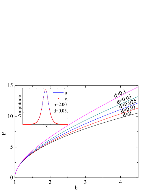
Figure 1.  : (Color online) Total power $P$ versus the soliton’s propagation constant, $b$, at different fixed values of the squared nonlocality correlation radius, $d$, for symmetric solitons in the model based on Eqs. (1). The inset shows a typical soliton profile. For the antisymmetric solitons, $b$ is shifted by $\Delta b=-2$. All quantities are plotted in arbitrary dimensionless units.

Proceeding to numerically found asymmetric solitons, in Fig. IV(a) we plot the respective $P(b)$ curves for for different fixed values of $d$. As in the local system, asymmetric modes appear through the SBB when the total power exceeds the threshold value, $P_{\mathrm{th}}$. Note that the threshold, as well as the value of the total power at the bifurcation point, $P=P_{\mathrm{bif}}$, significantly grow with $d$ [see Fig. IV(b)], in accordance with the prediction of the VA given by Eqs. (23) and (20). Further, the $P(b)$ curves change their shape with the growth of the nonlocality radius: At small $d$, the slope, $dP/db$, is initially negative (which definitely implies the instability, according to the VK criterion VK ), going over to $dP/db>0$ with the further increase of $b$. With the increase of $d$, the segment with the negative slope shrinks, and disappears at $d>0.05$.

The change in the shape of the $P(b)$ characteristics is directly related to the switch of the SBB from sub- to the supercritical type (in other words, the switch from the symmetry-breaking phase transition from the first to second kind) bifurcations , as shown in Fig. IV(c), where $P=P_{\mathrm{th}}$ determines the turning points of the $\Theta(P)$ curves, and their unstable portions with $d\Theta/dP<0$ precisely correspond to the segments with $dP/db<0$ in Fig. 2(b), both being confined to $P_{\mathrm{th}}<P<P_{\mathrm{bif}}$. Accordingly, the type of the SBB is subcritical, with $P_{\mathrm{th}}<P_{\mathrm{bif}}$ at $d<0.05$, and supercritical, with $P_{\mathrm{th}}\equiv P_{\mathrm{bif}}$, at $d>0.05$. The merger of $P_{\mathrm{th}}$ and $P_{\mathrm{bif}}$ into the single value at $d>0.05$ is clearly observed in Fig. IV(b). Recall that, as mentioned above, the trend to the merger of the two critical powers was predicted by the VA, see Eq. (27).

It is relevant to compare this result with the transition from the subcritical SBB for solitons into the supercritical bifurcation under the action of the periodic potential Warsaw . Although the models are very different (the one considered in Ref. Warsaw is local), a common feature is the introduction of a specific spatial scale—the nonlocality range in the present model, $\sqrt{d}$, or the lattice period in the local model—which is a factor accounting for the change of the character of the SBB.

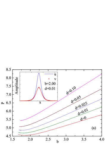
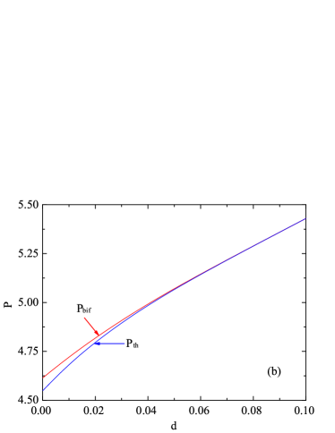
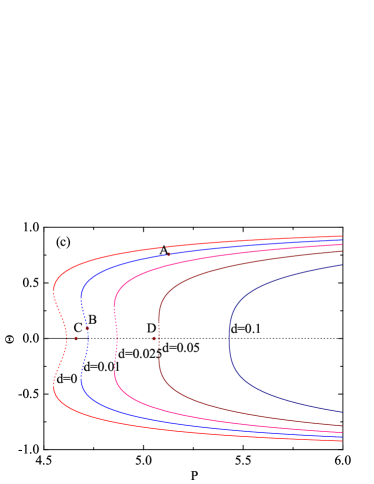
Figure 2.  : (Color online) (a) Total power $P$ versus propagation constant $b$ for asymmetric solitons at different values of the squared nonlocality radius, $d$. The inset shows a typical soliton profile. (b) The dependence on nonlocality $d$ of the total power, $P_{\mathrm{bif}}$, at which the symmetry-breaking bifurcation gives rise to asymmetric solitons, and of the threshold power, $P_{\mathrm{th}}$, at which the pair of stable and unstable asymmetric solitons emerge subcritically. (c) The bifurcation diagram accounting for the creation of the asymmetric solitons from the symmetric ones. In panels (a) and (c), dashed curves depict unstable portions of the asymmetric-soliton families [the border between stable and unstable (dashed) parts of the symmetric-soliton family in Fig. 2(c) corresponds to $d=0.01$]. All quantities are plotted in arbitrary dimensionless units.

The stability of the solitons was tested by means of systematic simulations of Eqs. (1), starting with perturbed initial conditions, $u(x,z=0)=U(x)(1+\rho(x)),v(x,z=0)=V(x)(1+\rho(x))$, where $U(x),V(x)$ is a stationary solution, and $\rho(x)$ is a small-amplitude random function. As expected, it has been found that the solid portions of the curves in Figs. IV(a) and IV(c), with $dP/db>0$ and $d\Theta/dP>0$, carry stable solitons, while the dashed segments, with $dP/db<0$ and $d\Theta/dP<0$, represent unstable solutions. Thus, the increase of the nonlocality radius, $\sqrt{d}$, gradually eliminates the instability region for the asymmetric solitons, making them completely stable in the case when the SBB is supercritical, i.e., at $d>0.05$.

It is relevant to explore the evolution of the two species of unstable solitons in the dual-core system, viz., asymmetric ones belonging to the segments of the $\Theta(P)$ curves with the negative slope [i.e., $\Theta<\Theta(P_{\mathrm{th}})$, that exist at $d<0.05$], which are represented, for example, by point B in Fig. IV(c), and symmetric solitons with $P>P_{\mathrm{bif}}$, sampled by point D in Fig. IV(c). Figure IV(a) displays the result for the unstable asymmetric soliton, which demonstrates long-lived oscillations, initiated by the instability, and eventual relaxation into a stable soliton with almost the same power but higher asymmetry, $\Theta>\Theta(P_{\mathrm{th}})$, which belongs to the stable branch of asymmetric modes in Fig. IV(c). Further, Fig. IV(b) demonstrates that the instability of the symmetric soliton leads to its spontaneous rearrangement into an asymmetric one, with nearly the same total power.

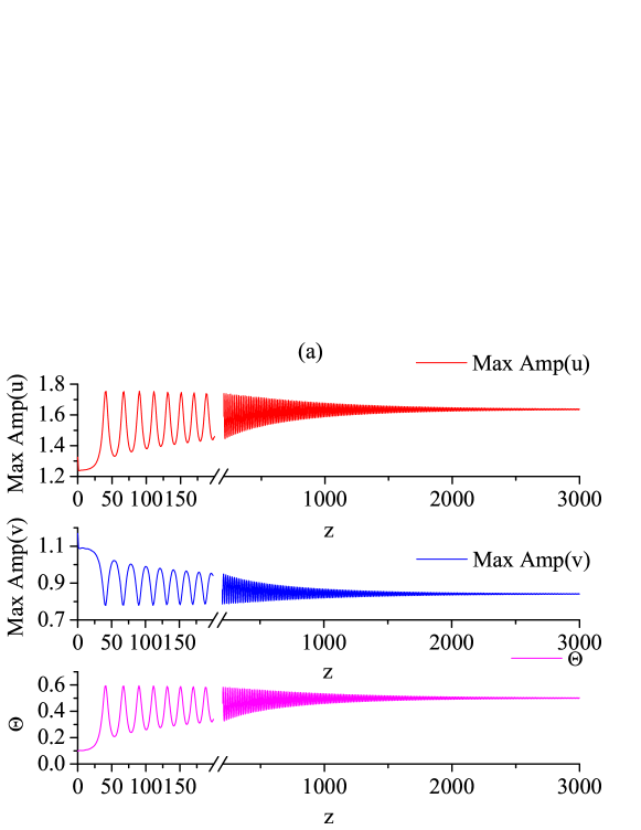
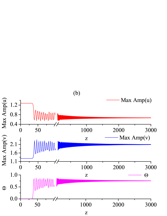
Figure 3.  : (Color online) (a,b): The evolution of perturbed unstable solitons corresponding, respectively, to points B and D marked in Fig. 2(c) (weakly asymmetric and symmetric solitons) is shown in terms of amplitudes of both components, and asymmetry measure (5). Both examples pertain to $d=0.01$. All quantities are plotted in arbitrary dimensionless units.

We have also studied the stability and evolution of antisymmetric solitons for different strengths of the nonlocality in the model based on Eqs. (1) (the stability of the antisymmetric solitons in the model of the coupler with the local nonlinearity was studied, in a numerical form, in Ref. anti ). In contrast to the asymmetric solitons, where the nonlocality leads to the transition from the subcritical SBB to the supercritical bifurcation, and thus enhances the stability of the asymmetric solitons, it has been found that the stability of the antisymmetric ones is weakly affected by the nonlocality: the stability region slightly expands under the action of the nonlocality, without dramatic changes.

V Conclusion

We have introduced the nonlocal generalizations of the standard model of the nonlinear directional coupler. The system can be built, in particular, as a dual-core optical waveguide made of a material with thermal nonlinearity. By means of the VA (variational approximation) and systematic numerical analysis, we have found that the relatively weak nonlocality shifts the SBB (symmetry-breaking bifurcation) of solitons to larger values of the total power, and eventually changes the character of the SBB from subcritical to the supercritical (i.e., the corresponding phase transition of the first kind goes over into the transition of the second kind). Thus, the nonlocality of the cubic nonlinearity enhances the stability for the asymmetric solitons, and eventually leads to their stabilization in the whole existence domain, while only slightly affecting the stability of antisymmetric solitons. For the consideration of the opposite case of the ultra-nonlocal nonlinearity, the coupler based on the SM (Snyder-Mitchell) model was introduced. In that case, the phase transition leads to the spontaneous breaking of the antisymmetry of the corresponding two-component “accessible solitons”. The exact transition point was found, and the strongly asymmetric states were found by means of the WKB approximation.

The analysis reported in this paper can be extended in other directions. In particular, as concerns nonlocal dual-core systems in other physical contexts, it may be quite interesting to study the SBB and asymmetric solitons in the case when the nonlocal interactions act between the cores, an important example being a two-layer dipolar BEC Santos . The symmetry-breaking point can be easily found for the respectively modified SM coupler model. A challenging extension is to construct two-dimensional solitons in dual-core systems, where they may be stabilized against the collapse by the nonlocality of the nonlinearity.

Acknowledgements

F. Ye acknowledges the support of the National Natural Science Foundation of China (Grant No. 10874119). B.A.M. appreciates hospitality of the Department of Physics at the Shanghai Jiao Tong University, and of the Department of Physics at East China Normal University (Shanghai).

References

- (1) S. M. Jensen, IEEE J. Quantum Electron. 18, 1580 (1982); A. M. Maier, Kvant. Elektron. (Moscow) 9, 2296 (1982) [Sov. J. Quantum Electron. 12, 1490 (1982)].
- (2) S. Trillo, S. Wabnitz, E. M. Wright, and G. I. Stegeman, Opt. Lett. 13, 672 (1988); S. R. Friberg, A. M. Weiner, Y. Silberberg, B. G. Sfez, and P. S. Smith, ibid. 13, 904 (1988).
- (3) F. Kh. Abdullaev, R. M. Abrarov, and S. A. Darmanyan, Opt. Lett. 14, 131 (1989).
- (4) E. M. Wright, G. I. Stegeman, and S. Wabnitz, Phys. Rev. A 40, 4455 (1989).
- (5) C. Paré and M. Fłorjańczyk, Phys. Rev. A 41, 6287 (1990).
- (6) A. W. Snyder, D. J. Mitchell, L. Poladian, D. R. Rowland, and Y. Chen, J. Opt. Soc. Am. B 8, 2101 (1991).
- (7) M. Romangoli, S. Trillo, and S. Wabnitz, Opt. Quantum Electron. 24, S1237 (1992).
- (8) W. C. K. Mak, B. A. Malomed, and P. L. Chu, J. Opt. Soc. Am. B 15, 1685 (1998); Phys. Rev. E 69, 066610 (2004); Y. J. Tsofe and B. A. Malomed, ibid. 75, 056603 (2007).
- (9) W. C. K. Mak, B. A. Malomed, and P. L. Chu, Phys. Rev. E 55, 6134 (1997); ibid. 57, 1092 (1998).
- (10) A. Gubeskys and B. A. Malomed, Phys. Rev. A 75, 063602 (2007); M. Matuszewski, B. A. Malomed, and M. Trippenbach, ibid. 75, 063621 (2007); L. Salasnich, B. A. Malomed, and F. Toigo, ibid. 81, 045603 (2010); N. V. Hung, M. Trippenbach, and B. A. Malomed, ibid. 84, 053618 (2011).
- (11) M. Trippenbach, E. Infeld, J. Gocalek, M. Matuszewski, M. Oberthaler, and B. A. Malomed, Phys. Rev. A 78, 013603 (2008).
- (12) A. I. Maimistov, Kvant. Elektron. 18, 758 [Sov. J. Quantum Electron. 21, 687 (1991)].
- (13) N. Akhmediev and A. Ankiewicz, Phys. Rev. Lett. 70, 2395 (1993).
- (14) P. L. Chu, B. A. Malomed, and G. D. Peng, J. Opt. Soc. Am. B 10, 1379 (1993).
- (15) J. M. Soto-Crespo and N. Akhmediev, Phys. Rev. E 48, 4710 (1993).
- (16) K. S. Chiang, Opt. Lett. 20, 997 (1995).
- (17) B. A. Malomed, I. Skinner, P. L. Chu, and G. D. Peng, Phys. Rev. E 53, 4084 (1996).
- (18) L. Albuch and B. A. Malomed, Mathematics and Computers in Simulation 74, 312 (2007).
- (19) G. Iooss and D. D. Joseph, Elementary Stability and Bifurcation Theory (Springer, New York, 1980).
- (20) B. A. Malomed, in: Progr. Optics 43, 71 (E. Wolf, editor: North Holland, Amsterdam, 2002).
- (21) A. W. Snyder and D. J. Mitchell, Science 276, 1538 (1997).
- (22) W. Królikowski, O. Bang, N. I. Nikolov, D. Neshev, J. Wyller, J. J. Rasmussen, and D. Edmundson, J. Opt. B: Quantum Semiclass. Opt. 6, S288 (2004).
- (23) W. Królikowski, O. Bang, J. J. Rasmussen, and J. Wyller, Phys. Rev. E 64, 016612 (2001); O. Bang, W. Królikowski, J. Wyller, and J. J. Rasmussen, ibid. E 66, 046619 (2002); W. Królikowski, O. Bang, J. J. Rasmussen, and J. Wyller, Opt. Exp. 13, 435 (2005).
- (24) C. Rotschild, O. Cohen, O. Manela, M. Segev, and T. Carmon, Phys. Rev. Lett. 95, 213904 (2005); C. Rotschild, B. Alfassi, O. Cohen, and M. Segev, Nature Physics 2, 769 (2006).
- (25) A. Dreischuh, D. N. Neshev, D. E. Petersen, O. Bang, and W. Królikowski, Phys. Rev. Lett. 96, 043901 (2006).
- (26) C. Conti, M. C. Conti, M. Peccianti, and G. Assanto, Phys. Rev. Lett. 91, 073901 (2003).
- (27) C. Conti, M. Peccianti, and G. Assanto, Phys. Rev. Lett. 92, 113902 (2004).
- (28) D. Suter and T. Blasberg, Phys. Rev. A 48, 4583 (1993).
- (29) S. Skupin, M. Saffman, and W. Królikowski, Phys. Rev. Lett. 98, 263902 (2007).
- (30) F. Ye, Y. V. Kartashov, and L. Torner,solitons in nonlocal nonlinear media, Phys. Rev. A 77, 043821 (2008).
- (31) J. H. Huang and R. L. Chang, J. Optics 12, 045003 (2010); M. Wand, A. Schindlmayr, T. Meier, and J. Forstner, Physica Status Solidi B 248, 887 (2011); S. Thongrattanasiri, A. Manjavacas, and F. J. G. de Abajo, ACS NANO 6, 1766 (2012).
- (32) D. Mihalache and D. Mazilu, Romanian Reports in Physics 61, 235 (2009).
- (33) H. L. Pécseli, and J. J. Rasmussen, Plasma Physics Contr. Fusion 22, 421 (1980).
- (34) L. A. Rivlin, Quantum Electron. 28, 99 (1998).
- (35) T. Lahaye, C. Menotti, L. Santos, M. Lewenstein, and T. Pfau, Rep. Progr. Phys. 72, 126401 (2009).
- (36) D. O’Dell, S. Giovanazzi, G. Kurizki, and V. M. Akulin, Phys. Rev. Lett. 84, 5687 (2000); S. Giovanazzi, D. O’Dell, and G. Kurizki, Phys. Rev. A 63, 031603 (2001); I. Papadopoulos, P. Wagner, G. Wunner, and J. Main, ibid. 76, 053604 (2007).
- (37) M. Peccianti, K. A. Brzdakiewicz, and G. Assanto, Opt. Lett. 27, 1460 (2002).
- (38) V. M. Perez-Garcia, V. V. Konotop, and J. J. Garcia-Ripoll, Phys. Rev. E 62, 4300 (2000).
- (39) O. Bang, W. Królikowski, J. Wyller, and J. J. Rasmussen, Phys. Rev. E 66, 046619 (2002).
- (40) F. Ye, Y. Kartashov, B. Hu, and L. Torner, Opt. Lett. 35, 628 (2010).
- (41) F. Ye, L. Dong, and B. Hu, Opt. Lett. 34, 584 (2009).
- (42) R. Nath, P. Pedri, and L. Santos, Phys. Rev. A 76, 013606 (2007).
- (43) C.-F. Huang and Q. Guo, Opt. Commun. 277, 414 (2007); Q. Kong, M. Shen, J. L. Shi, and Q. Wang, Phys. Lett. A 372, 244 (2008); Y. J. He, B. A. Malomed, D. Mihalache, H. Z. Wang, Phys. Rev. A 77, 043826 (2008); I. B. Burgess, M. Peccianti, G. Assanto, and R. Morandotti, Phys. Rev. Lett. 102, 203903 (2009); F. Maucher, D. Buccoliero, S. Skupin, M. Grech, A. S. Desyatnikov, and W. Królikowski, Opt. Quant. Electr. 41, 337 (2009); W. P. Zhong, M. Belić, R. H. Xie, T. W. Huang, and Y. Lu, Opt. Commun. 283, 5213 (2010).
- (44) A. Butsch, C. Conti, F. Biancalana, and P. St. J. Russell, Phys. Rev. Lett. 108, 093903 (2012).
- (45) W. Królikowski and O. Bang, Phys. Rev. E 63, 016610 (2000).
- (46) M. Vakhitov and A. Kolokolov, Radiophys. Quantum. Electron. 16, 783 (1973); L. Bergé, Phys. Rep. 303, 259 (1998); E. A. Kuznetsov and F. Dias, ibid. 507, 43 (2011).