A Method for the Characterisation of Observer Effects and its Application to OML

Abstract

In all measurement campaigns, one needs to assert that the instrumentation tools do not significantly impact the system being monitored. This is critical to future claims based on the collected data and is sometimes overseen in experimental studies. We propose a method to evaluate the potential “observer effect” of an instrumentation system, and apply it to the OMF Measurement Library (OML). OML allows the instrumentation of almost any software to collect any type of measurements. As it is increasingly being used in networking research, it is important to characterise possible biases it may introduce in the collected metrics. Thus, we study its effect on multiple types of reports from various applications commonly used in wireless research. To this end, we designed experiments comparing OML-instrumented software with their original flavours. Our analyses of the results from these experiments show that, with an appropriate reporting setup, OML has no significant impact on the instrumented applications, and may even improve some of their performances in specifics cases. We discuss our methodology and the implication of using OML, and provide guidelines on instrumenting off-the-shelf software.

^⋆Corresponding author: olivier.mehani@nicta.com.au
¹first.last@nicta.com.au MSWIM 2012, May 13, 2012 TR-5895 Submitted to MSWIM 2012

1 Introduction

Measurement is a foundation stone of scientific research. It is the analysis of measured data that allows researchers to support or refute scientific claims. Many types of data can be collected using tools with various characteristics in accuracy, precision, and impact on the systems under study. Without characterising these measurement tools, it is impossible to assess the validity of the conclusions that are based on the collected data.

Networking technologies are closely linked to the software system that embodies and controls them. Many of the tools used to observe networking behaviours consist in software executing alongside the systems under study, on the same machine and operating environment. If not designed carefully, such tools may alter the system’s performance or functionality, which in turn may impact the observations being made. It is therefore important to characterise the “observer effect” that an instrumentation software tool has on a networking system. This step is sometimes overseen in experimental studies.

When designing an experiment, a researcher often has to collect measurements from multiple sources involved in the study. In wireless networking, this usually involves a combination of various third-party and home-brew software tools to measure and report the data. OML is an open source measurement framework, which facilitates these two phases by allowing an experimenter to collect any type of measurements from many types of software, and store them in a unified format for future analysis [26]. It is composed of a client library and a collection server. The client library is used to instrument any software from which a researcher would like to collect measurements. It can apply some processing (i.e., filter) to the samples on the fly, then streams them to a collection server, which stores them in a database along with measurements from other elements involved in the experiment. An increasing number of researchers from various institutions have used OML in their wireless studies [17, 3].

Our objective in this paper is to characterise the observer effect that OML has on the software that it instruments. To this end, we selected two types of widely used software, a network probing tool (Iperf [9]) and a packet capture library (libtrace [1]). We instrumented them using OML and compared many indicator variables between the instrumented and vanilla flavours to detect any significant impact that the OML instrumentation could have on the software.

Our contribution is twofold. First, we propose a methodology to characterise the observer effect of a networking measurement framework. This methodology and its specific application, in this paper, to OML are described in Section 2. Second, we identify the cases where OML introduces statistically significant deviations in the performance of instrumented applications, and those where no impact can be detected. This demonstration is based on the analysis of the indicator variables selected for each instrumented tool, and is presented in Section 3. We believe that this contribution is novel and relevant as few other works thoroughly study the observer effect of measurement frameworks, and OML’s use is growing within the wireless research community. We further discuss the findings and limitations of our study in Section 4, then present some related work in Section 5, and finally conclude this paper in Section 6.

2 Methodology

2.1 Objectives

Our objective is to test whether using OML version 2.6.1 to instrument a piece of software for a networking study has any impact on its behaviours and observed performance. If there were, this could alter the variables being measured in the study. In other words, we would like to demonstrate that the “observer effect” of OML is negligible. What we define as an impact is a statistically significant deviation in some performance indicators between the original software and other OML-instrumented flavours.

While several researchers have used OML to instrument many software tools, we limit this study to two of them, namely the Iperf network probing application [9] , and the libtrace [1] packet capture library. It is not the purpose of our study to evaluate the accuracy or precision of these tools. Rather, we are only interested in possible deviations introduced by the use of OML instead of their original reporting channels.

We propose the following four-step method to characterise the observer effect of OML.

1. formulation of the objective and selection of the material to use;

2. design of the experiment, which includes the formulation of the hypotheses, the identification of the factors which may influence these hypotheses and the dependent variables to measure in order to test them; the description of the experiment setup is also considered there;

3. the analysis of the measured variables, using statistical tools which are adequate to the nature of the selected factors and variables;

4. the discussion on the conclusions from the results of step 3, and the limitations of step 2, which may lead to further study via another iteration of step 1.

2.2 Materials

2.2.1 OML

OML [26] is a distributed, open source, and multithreaded measurement framework. It provides a client library, which can be used to instrument any piece of software. An instrumented application “injects” its samples to the library for processing and streaming to at least one collection server. When requested by the software’s user, this client library may apply some processing filters to the measurements before forwarding them. The collection server receives the samples from software running on all nodes involved in a given experiment (identified by a unique ID), and store them in a timestamped database with a unified format.

OML has an active user community, which has contributed to the instrumentation of a wide range of software used in networking research, such as the radiotap library (802.11 frame characteristics), wlanconfig (driver status), but also applications such as VLC (media streaming) or btclient (BitTorrent client).

Within an experiment, each OML-instrumented software generates a timestamp (oml_ts_client) for each generated sample. The receiving server rebases this timestamp to a local origin (oml_ts_server), i.e., the time of the first connected client for that experiment. This allows for low-resolution ($\sim$1 s) comparisons and correlations between measurements from different sources. Since the client and rebased timestamps are both stored in the database, a high-resolution comparison can also be achieved by deploying a separate synchronisation scheme such as [25] on all clients.

To instrument an application with OML, a developer first defines one or many measurement points (MPs) within its source code. An MP is an abstraction for a tuple of related metrics to be reported at the same instant. Thus the MPs define all the potential measurements that the application can report. The modified source code is then compiled against the OML client library to generate the OML-instrumented software. At run-time, the experimenter can request some or all of the defined MPs to generate measurement streams (MSs). This is done through an XML configuration file passed to the software at startup.

Prior to streaming MSs to a server, the client library may apply predefined filters to the samples, as described in the XML configuration file. This filtering process is illustrated in Figure 1. Filters are composable functions, which are applied to a subset of metrics from MSs over a given time or sample period (e.g., every 1 s or 10 samples). Thus they integrate incoming MSs into newly generated outgoing MSs. OML has some built-in filters and allow users to create custom ones. Examples of simple OML filtering capabilities include averaging a metric over a time window, or getting its extreme values (min/max) over a given number of samples.

Figure 1: Measurement data path in OML: Three MPs are filtered to generate MSs which get sent for storage at different locations.

OML clients stream MSs to the servers over TCP using a custom protocol. They have a finite-sized outgoing buffers and may therefore drop some measurement samples if the path to the server cannot provide sufficient capacity to cater for the sample rate. A sequence ID incremented for every sample allows the detection of such events on the server side.

2.2.2 Network Probing with Iperf

Iperf [9] is a versatile open source active network probing tool. It allows an experimenter to test the characteristics of a network path using either TCP or UDP. Its code is multithreaded to limit the impact of reporting—either on the console or in a CSV file—on the high-speed generation of probe packets.

Iperf can report a number of metrics depending on the transport protocol in use. For TCP only the transferred size, from which the throughput is derived, can be observed. For UDP, packet loss and jitter information can also be reported. The periodicity of Iperf’s reports is configurable from once for an entire run to every half a second. The internal aggregation function depends on the metric: the transferred size and losses are summed, while the latest value to date is reported for the jitter.

There tends to be some confusion with the definition of jitter [8]. In the case of Iperf, the term refers to the variation in packets transit times, as proposed in [23], and it is computed at packet $p$ as

$$\tau_{p}=t_{p}^{Rcv}-t_{p}^{Snd}$$

$$\Delta\tau_{p}=|\tau_{p}-\tau_{p-1}|$$

$$J_{p}=J_{p-1}+\frac{1}{16}(\Delta\tau_{p}-J_{p-1}).$$ (1)

As this jitter itself is based on the variation of transit times, rather than the immediate values, it is rather robust to loose time synchronisation between sender and receiver.

We have instrumented version 2.0.5 of Iperf to support reporting via OML. We implemented two new additional forms of measurement reporting styles, legacy (iperf -y o) and advanced (iperf -y O), which differ in the amount of processing that is done in the application. Table 1 summarises the performance metrics directly reported by the different flavours of Iperf used in this study.

Table 1: Metrics reported by the various Iperf flavours in this study

Flavour	Reported metrics (for UDP traffic)
Vanilla	Transferred size, throughput, losses, jitter
OML legacy	Transferred size, throughput, losses, jitter
OML advanced	Packet ID, size, emission and reception
	timestamps

In the legacy mode, the aggregation of the measurements is done using Iperf’s standard code, and the periodic reports are sent out through OML via three MPs: transfer for the size, losses for lost and sent datagrams, and jitter for Iperf’s implementation of (1). In the advanced mode, Iperf directly reports information about each packet sent or received via OML, in the packets MP which contain identification, size and both sent and received (if relevant) times for each packet, down to the microsecond. The advanced mode is more in line with OML’s approach, where the measured data is reported verbatim by the application and all processing and consolidation is done through filters, thus allowing more experiment-specific treatment without impacting the main operation of the application. Noting that, in most of the literature using Iperf, there is a lack of precise reporting of versions, platforms and parameters, we also implemented MPs to report such ancillary information about the experiment as the version numbers and command line arguments.

2.2.3 Packet Capture with libtrace

Packet capture in networking environments is usually done via wrapper libraries hiding the operating system’s underlying API. Perhaps the most common libraries for this purpose are libpcap and libtrace [1]. The latter offers a broader range of input and output APIs and formats than the former.

We implemented trace-oml2, a simple packet-capturing application which uses libtrace to get packet header information from the kernel. This data is then available from trace-oml2’s MPs, and can be collected using OML as required by the experimenter. Table 2 lists the available metrics from the packet headers, and trace-oml2’s MPs providing them. As previously, we need to consider different flavours of this application, and also implemented an almost identical trace-nooml, which reports the metrics in a local CSV file rather than through OML, by modifying the reporting functions.

Table 2: Measurement Points & Metrics available from trace-oml2.

MP name	Reported metrics
radiotap	Seq. ID, MAC addresses, & other MAC fields
ip	Pkt ID, IP addresses, length, & other IP fields
tcp or udp	ID, length, ports, and other transport fields
All MPs	Timestamp

2.3 Experimental Design

To achieve our goal (section 2.1), we compare some performance indicators between the original and OML instrumented flavours of Iperf and our libtrace-based tool. In addition, we also quantify the impact of the forwarding of MSs on other experiment-generated traffic in a shared wireless environment. Thus, we design and perform three sets of experiments, one focusing on Iperf, another on libtrace, and the last one on the impact of reporting traffic.

The two first sets are based on a simple 2-hop topology composed of a sender ($Snd$), a router ($Rtr$; with an ingress $RtrIn$ and egress $RtrEg$ interfaces), and a receiver ($Rcv$). Within each set of experiments, we vary some specific setup parameters, such as the flavour of the tool under study (e.g., vanilla or OML-instrumented with feature $X$ enabled). These parameters are our study’s independent variables (or factors). For each experiment trial, we measure some performance indicators such as the sending rate or report accuracy, which are our study’s dependent variables. In these two sets, the measurement streams are sent to an OML server on a separate network from the experiment-generated traffic, and thus do not impact it.

The third set involves a sender ($Snd$) generating traffic towards a a receiver ($Rcv$). The same OML-instrumented tools as previously are used to collect measurements. However, in this set the measurement streams are sent to an OML server over the same wireless channel as the generated traffic between $Snd$ and $Rcv$.

2.3.1 Experiment Set 1

This set aims at characterising the effect of OML on the performance of Iperf. We are specifically interested in how Iperf’s traffic generation and the accuracy of its traffic statistic reports may be altered by the OML instrumentation. Thus our working null hypothesis for this first set is: “the OML instrumentation of Iperf has no significant effect on its packet-sending rate nor on the accuracy of its throughput and jitter reports.”

Experimental Factors

Many factors may influence the performance or accuracy of Iperf. For this first set, we restrict our experimental design to three factors. The first factor is the Iperf flavour being used. Indeed, the use of OML and its various features introduce some processing overheads on Iperf, which may deteriorate performance and report accuracy, as compared to the original Iperf. We consider the following values for this factor:

nooml

the original Iperf, reporting to a CSV file

o

OML-enabled Iperf, reporting metrics computed by Iperf (the same as the original version)

O

OML-enabled Iperf, reporting information on all sent/received packets

Of

OML-enabled Iperf, reporting metrics computed by OML filters

The second factor we are interested in is the set rate at which Iperf is instructed to generate the experimental traffic. At high rates, the per-packet instrumentation processing may take longer than the inter-packet sending interval, thus impeding the actual sending rate. Although the sending rate is a continuous variable, for the purpose of our study we are only interested in given rate values, and thus treat it as a fixed factor with the values: 10, 50, 75, 100, 200 and 300 Mbps.

The last factor is the use of threads. The original Iperf has the option to use threads or not to report traffic information out of the main traffic generation loop. In our study, this feature may mask the effects introduced by the OML-instrumentation. Thus we consider two values, threads and nothreads.

Response Variables

In this set of experiments, we decide to measure the following three dependent variables, which we will use in the next section to test our working hypothesis. First, we measure the actual sending rate ($R_{t}^{RtrIn}$) of the sending Iperf as computed from tcpdump traces ($t$) on the router’s ingress link from the sender.

We also measure the accuracy of the throughput report ($T_{Diff}^{Rcv}$) of the receiving Iperf, which is the difference between the throughput as reported by the receiving Iperf ($i$) and the computed throughput from tcpdump traces on the router’s egress link to the receiver. For a given sample, $T_{Diff}^{Rcv}=R_{t}^{RtrEg}-T_{i}^{Rcv}$.

Finally, we measure the jitter report accuracy ($J_{Diff}$) of the receiving Iperf, which is the difference between the jitter as reported by the receiving Iperf and the computed jitter using equation (1) on the tcpdump traces on the router’s egress link to the receiver. For given sample, we have $J_{Diff}=J_{i}^{Rcv}-J_{t}^{RtrEg}$.

2.3.2 Experiment Set 2

The goal of this set is to evaluate the effect of OML on the a tool based on the libtrace packet-capture library. We are particularly interested in finding out if the OML instrumentation degrades the accuracy of the packet and timestamp reports from libtrace. Thus our working null hypothesis in this case is: “the OML instrumentation of libtrace has no significant effect on the accuracy of its packet and timestamp reports.”

Experimental Factors

As in the previous experiment set, the first obvious factor that may impact the accuracy of libtrace’s reports is the librace application flavour being used. Here we only consider the two simple cases where libtrace is used with and without OML instrumentation, i.e., trace-oml2 (oml) and trace-nooml (nooml). In the former case, we also consider the use of a summation filter (Of) on the length field of the IP header (ip_len).

Similarly, the second factor that we consider is the set rate for the traffic generation between the sender and the receiver. Indeed, increased packet rate may translate in increased instrumentation processing for packet reporting on the receiver. This may result in received packets not being reported in the measurement file, as they are dropped by the instrumentation mechanism being overwhelmed by the high packet rate. For this factor, we use the same fixed rates as in the first experiment set, 10, 50, 75, 100, 200 and 300 Mbps.

Response Variables

We measure three dependent variables in this experiment set. The first one is the accuracy of packet reports, in the form of losses ($L^{Rcv}$), generated by our libtrace-based tool at the receiver. This is the ratio between the number of packets sent to the receiver as counted from tcpdump traces on the router’s egress link ($N_{t}^{RtrEg}$) to that of the packets reported by the receiver’s instrumentation ($N_{i}^{Rcv}$). Thus for a given sampling window, we have $L^{Rcv}=1-N_{i}^{Rcv}/N_{t}^{RtrEg}$.

Closely related to the previous one, we also consider the accuracy of received rate by computing it based on the ip_len field of the reported packets, $R^{Rcv}=\sum_{0}^{N}\mathtt{ip\_len}$.

Our last measured variable is the accuracy of timestamp reports ($t_{Diff}^{Rcv}$). For a given packet this is the difference between the timestamp from the tcpdump traces and the one from the libtrace report at the receiver, $t_{Diff}^{Rcv}=t_{t}^{Rcv}-t_{i}^{Rcv}$.

For the first and second set of experiments, we would like to stress that we are only interested in the relative differences in our dependent variables in response to our independent factors (e.g., OML instrumentation), rather than their absolute “true” values. Indeed, running many measurement tools on a machine (e.g., libtrace and tcpdump on the receiver) will probably introduce biases in the absolute measured value of performance or accuracy. However, we compare the differences between runs where only our above factors vary and all others parameters remain identical. Thus these biases have the same occurrence probability across runs, and deriving claims on the analysis of the variances from these runs is scientifically sound.

2.3.3 Experiment Set 3

This set aims at quantifying the effect of the OML measurement traffic on the experiment-generated traffic, when they both share the same wireless channel. In this case, an impact is indeed expected as both types of traffic contend for the same medium. In this set of experiments, we are interested in characterising how the experiment traffic varies as a function of the amount of collected measurement.

The first factor in this set is the OML sampling rate, which is the frequency (per sample) at which an OML-instrumented libtrace (trace-oml2) generates an aggregated report and sends it to the server. We vary this factor in the range $\mathsf{1}$, $\mathsf{\frac{1}{10}}$, $\mathsf{\frac{1}{50}}$, and $\mathsf{\frac{1}{100}}$—the higher the sampling rate, the higher the number of measurements forwarded to the server. The second factor considered is the packet size that Iperf uses as the MTU for the experimental wireless path. Two values are considered, 1,500 and 1,000 B, in order to explore the impact of a varying number of packets on the same theoretically achievable throughput.

We measure a single dependent variable, which is the achieved throughput as reported by an OML-instrumented Iperf in legacy mode on the receiver.

2.4 Experiment Execution

In the first two sets, all experiments were performed on a testbed where the nodes are all recent machines. Two separate Intel Pro/1000 Gigabit LAN interfaces carried the experimental traffic on one side and the control and measurement traffic on the other. This ensured that neither the control and measurement traffic nor the performance capability of the machines biased our experiments. UDP was used to transport the experimental traffic to be able to analyse jitters.

For the third set, we used a wireless testbed similar to ORBIT [22]. The wireless nodes were connected via an 802.11g adhoc network, which carried both experimental and measurement traffic. TCP was used to transport the experiment traffic as this is what OML streams use, thus avoiding any potential TCP/UDP interaction bias. The detailed specifications of these nodes can be found in [18].

All our experiments were performed using the OMF framework [21] on the IREEL experimentation portal [14]. Their precise descriptions are available and can be used to reproduce them on any OMF-enabled testbeds.

3 Results

This section presents the results of the analyses which we performed on the collected experimental data. All of the measurement data collected from our sets of experiments are available online with the R scripts used to analyse them.

In each 5 mn run, we collected 600 aggregate samples (one every half-second) for each specific parameter cases in each experiment set, to mitigate any unforeseen random factor. The sample times where rebased to 0 in their respective timeframe to allow for meaningful comparisons between sources. The first and last samples of each data sets were ignored to avoid bias due to incomplete measurement periods at startup and teardown.

3.1 Analysis and Assumptions

An Analysis of Variance (ANOVA) is the established analysis for comparative studies where the factors have categorical levels and the dependent variables are continuous. This is our case, as described in Section 2.3. Thus, we performed a series of ANOVAs on our collected data and attempt to disprove our null hypotheses by identifying significant variations between each cases in our experimental sets. We set our significance level $\alpha=0.05$ to have 95 % confidence when finding significant differences. We note that some of the ANOVA assumptions are not always met by our data, and address them as follows.

3.1.1 Independence of samples

As the samples of each variables for one trial come from a time series, they are clearly not independent, which is confirmed by Turning points tests [19]. We therefore make our data iid by sampling it randomly with replacement as suggested in [16].

3.1.2 Homoskedasticity

In some cases, Breusch-Pagan tests show that the variance of our samples differs significantly between treatment groups. Studies have however showed that the ANOVA is robust to deviations from this assumption at the price of a small reduction of the confidence $1-\alpha$ and an increase of the power of the test $\beta$ [11, 13]. Moreover, we note that these studies focused on ratio of variances only as low as 1:2. Even in our extreme cases, computing the ratio of the variances reveals that the heteroskedasticity is much more modest than the cases studied in [11, 13]. We therefore conclude that our performed ANOVAs gave us valid results even with this caveat on the confidence.

3.1.3 Normality

This is the assumption from which our data deviated the most, both in terms of skewness and kurtosis. We characterised this deviation with a Shapiro-Wilk test for each treatment group and proceeded with an ANOVA if the deviation was not found to be significant. In case of significant deviations, we used a non-parametric version of the ANOVA which removes the normality assumption by creating an empirical null distribution through permutation of the samples throughout treatments [2].

3.2 Experiment Set 1 (Iperf Instrumentation)

We performed two-way ANOVAs with interactions for each of the variables $R_{t}^{RtrIn}$, $T_{\mathrm{Diff}}^{Rcv}$ and $J_{\mathrm{Diff}}$ at each of the studied set rates. Characteristic results are presented below.

3.2.1 Actual Sending Rate

The results of the ANOVA for Iperf’s sending rate as measured by an un-instrumented tcpdump, $R_{t}^{RtrIn}$, at rates 10, 100  and 300 Mbps are shown in Table 3 (left). The results of the analysis for set rate 50 are similar to those for 10, while those for 75, and 200 Mbps are similar to those for 100.

Table 3: Two-way PERMANOVAs with interactions on the actual sending rate of Iperf, $R_{t}^{RtrIn}$ (left), and the difference $T_{\mathrm{Diff}}^{Rcv}$ between the actual received rate and Iperf’s throughput report (right).

		$R_{t}^{RtrIn}$					$T_{\mathrm{Diff}}^{Rcv}$
	d.f.	$SS$	$MS$	$F$	$p$	Signif.	$SS$	$MS$	$F$	$p$	Signif.
	10 Mbps
oml	$3$	$2.69\times 10^{6}$	$8.97\times 10^{5}$	$1.76$	$0.17$	–	$1.12\times 10^{8}$	$3.72\times 10^{7}$	$0.95$	$0.42$	–
threads	$1$	$9.86\times 10^{5}$	$9.86\times 10^{5}$	$1.94$	$0.17$	–	$1.19\times 10^{7}$	$1.19\times 10^{7}$	$0.30$	$0.62$	–
oml:threads	$3$	$2.07\times 10^{6}$	$6.89\times 10^{5}$	$1.35$	$0.26$	–	$4.13\times 10^{7}$	$1.38\times 10^{7}$	$0.35$	$0.83$	–
	100 Mbps
oml	3	$6.15\times 10^{10}$	$2.05\times 10^{10}$	$0.81$	1.00	–	$8.81\times 10^{8}$	$2.94\times 10^{8}$	0.12	$1.00$	–
threads	1	$4.68\times 10^{10}$	$4.68\times 10^{10}$	1.85	0.001	$\star\star\star$	$7.21\times 10^{8}$	$7.21\times 10^{8}$	0.29	$0.85$	–
oml:threads	3	$9.85\times 10^{10}$	$3.28\times 10^{10}$	1.30	0.001	$\star\star\star$	$2.69\times 10^{9}$	$8.96\times 10^{8}$	0.36	$0.65$	–
	300 Mbps
oml	$3$	$4.00\times 10^{16}$	$1.33\times 10^{16}$	$2.45\times 10^{4}$	0.001	$\star\star\star$	$1.65\times 10^{15}$	$5.50\times 10^{14}$	$3.79\times 10^{3}$	0.001	$\star\star\star$
threads	$1$	$8.76\times 10^{14}$	$8.76\times 10^{14}$	$1.61\times 10^{3}$	0.001	$\star\star\star$	$1.69\times 10^{14}$	$1.69\times 10^{14}$	$1.16\times 10^{3}$	0.001	$\star\star\star$
oml:threads	$3$	$2.60\times 10^{15}$	$8.65\times 10^{14}$	$1.59\times 10^{3}$	0.001	$\star\star\star$	$4.78\times 10^{14}$	$1.59\times 10^{14}$	$1.10\times 10^{3}$	0.001	$\star\star\star$
Significance level: $\star\ 0.05$, $\star\star\ 0.01$, $\star\star\star\ 0.001$

For rates 75 Mbps and higher, there are statistically significant differences in Iperf’s sending rates, which are introduced by changes in both the use of threads and OML instrumentation, as well as the interaction of those two factors. When significant, this interaction has to be studied first, which we do in Figure 2 for case 300 Mbps. This figure shows the means of the response variable. It shows an interaction between the threads and oml factors. The O factor introduces a sizable negative impact, which is only partially mitigated by Iperf’s native threads. However, the use of filters in the Of factor completely removes the issue.

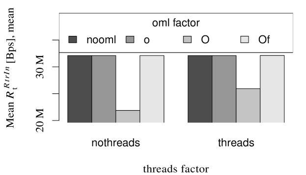
Figure 2: Sender rate $R_{t}^{RtrIn}$ achieved for different combinations of the experimental factors on at 300 Mbps. While advanced OML appears to have a negative impact, it is partially mitigated by Iperf’s internal threading, and fully removed by the use of OML filters (see Table 4).

The Tukey Honest Significant Differences test allows us to quantify the deviations observed in Figure 2. We present the relevant results allowing to characterise the previous figure in Table 4. For legibility’s sake, we only show the mean differences and the $p$-values. We however include all the differences between interactions which were found to be significant.

Table 4: Tukey Honest Significant Differences for oml:threads interactions with significant differences in the sending rate at 300 Mbps. All differences found significant ($p\leq 0.05$) are shown.

oml:threads interaction	diff	$p$ adj	Signif.
	[MBps]
O:nothreads–nooml:nothreads	-$10.2$	$0.00$	$\star\star\star$
O:threads–nooml:nothreads	-$6.08$	$0.00$	$\star\star\star$
O:nothreads–Of:nothreads	-$10.2$	$0.00$	$\star\star\star$
O:threads–Of:nothreads	-$6.08$	$0.00$	$\star\star\star$
O:nothreads–o:nothreads	-$10.2$	$0.00$	$\star\star\star$
O:threads–o:nothreads	-$6.08$	$0.00$	$\star\star\star$
nooml:threads–O:nothreads	$10.2$	$0.00$	$\star\star\star$
Of:threads–O:nothreads	$10.3$	$0.00$	$\star\star\star$
o:threads–O:nothreads	$10.2$	$0.00$	$\star\star\star$
O:threads–O:nothreads	$4.17$	$0.00$	$\star\star\star$
O:threads–nooml:threads	-$6.08$	$0.00$	$\star\star\star$
O:threads–Of:threads	-$6.09$	$0.00$	$\star\star\star$
O:threads–o:threads	-$6.08$	$0.00$	$\star\star\star$
Significance level: $\star\ 0.05$, $\star\star\ 0.01$, $\star\star\star\ 0.001$

Table 4 confirms the observations from Figure 2. Using OML to report every packets (O) has a significant impact on the sending rate, reducing it by an average (at most) 10.3 MBps at set rate 300 Mbps (about 27.5%). Iperf’s internal threads can reduce this difference by 4.17 MBps, which is still a 16.3% drop from the performance for the other treatments. Interestingly, though it is not found significant here, the use of OML filters in the Of treatments consistently enabled a slight increase in the sender’s rate as compared to vanilla Iperf (nooml treatment).

Next, we follow up with similar analyses for the other dependent variables we are considering. However, due to space constraints, we report subsequent results mostly in the text.

3.2.2 Accuracy of Throughput Reports

Here, we assess the variations of $T_{\mathrm{Diff}}^{Rcv}$ between the treatment groups, as an evaluation of the impact of the instrumentation on the accuracy of Iperf’s report. Table 3 (right) presents the corresponding ANOVA results.

At rates 10–200 Mbps, no statistically significant ($p>0.05$) difference can be found. Only for set rate 300 Mbps do important ($p\leq 0.05$) deviations in the mean appear. The combination of the oml and threads factors is, once again, studied first. The interaction between factors is qualitatively similar to Figure 2. Tukey HSD tests confirm that the treatment causing this deviation is also the non-filtered advanced mode (O) in both threads and nothreads treatments. No other difference in mean between other treatments (particularly nooml and Of) is found to be significant.

3.2.3 Accuracy of Jitter Reports

We finally attempt to find differences in $J_{\mathrm{Diff}}$ in a similar fashion. As OML does not currently provide a jitter-computing filter, we could not consider treatment Of in this case. For treatment O, we post-processed the packet records based on their arrival times to compute (1).

For rates 10 and 50 Mbps, no significant difference in the means could be found (p>0.05). For rates 75 Mbps and higher, however, the analyses of variance identified statistically significant ($p\leq 0.05$) deviations. They were always linked to the Iperf advanced mode (O), in comparison to the vanilla and legacy report modes.

This difference can be explained in a similar fashion as for the throughput reports where, with an increasing number of packets not being reported, the computed metric loses accuracy. A jitter-computing filter for OML would address this issue in the same way as the sum filter did in the previous section.

3.3 Experiment Set 2 (libtrace Instrumentation)

We performed a similar analysis on the relevant dependant variables of our packet-capture experiment. Characteristic results are reported thereafter.

3.3.1 Accuracy of Packet Reports

In this experiment, we are first interested in the loss ratio $L^{Rcv}$. In all treatments of the rate factor (200–300 Mbps), the OML-instrumented packet-capture application’s reports deviate in a statistically significant manner ($p\leq 0.001$) from the non instrumented version. We recall that this application reports two samples (ip and udp) per captured packet. With packets of size 1,498 B, this induces a rate between 6,675 and 200,267 pps, and double the number of samples. On average, 7.75 pps went unreported at 10 Mbps (1.42 %), but this went up to 216 pps at 300 Mbps (0.9 %).

As no loss filter is currently available for OML, only the nooml and oml treatments were studied for the oml factor. Considering the reported rate $R^{Rcv}$, as computed by summing the IP length of the reported factors allows to provides some insight nonetheless. As for the losses, the throughput exhibited significant differences ($p\leq 0.001$) depending on whether it was computed from trace-nooml or trace-oml2’s reports, with the latter being consistently lower (between 0.09 and 2.21 %). However, complementing the use of trace-oml2 with a summing filter (Of) produces statistically significant ($p\leq 0.001$ for treatments 75–300 Mbps) positive differences. We hypothesise that limiting processing in the main thread and reducing the number of report packets to be sent allowed for more packets to be read on time from the packet capture buffers, resulting in an increase in the reported throughput by 0.15–0.85 % depending on the cases. These observations are consistent with the Iperf results from the previous section.

3.3.2 Timestamp Accuracy and Precision

The trace-nooml tool does not compute a local timestamp as OML does for trace-oml2. It is therefore not possible to obtain $t^{Rcv}_{Diff}$ in the nooml case for comparison. Rather, we only consider the oml treatment. and give summary statistics for $t^{Rcv}_{Diff}$. They are summarised in Table 5. For rate 100 Mbps and below, the time difference is almost neglectable, with a maximum at 0.47 $\mu$s, and a mean of about 100 ns. It is interesting to note that some minimal differences are negative, which would hint that slightly different clocks are involved in the kernel-land timestamping of PCAP packets and OML’s userland gettimeofday(3) requests.

Set rate	$t^{Rcv}_{Diff}$ [s]
[Mbps]	min.	med.	avg.	max.	sd
10	-7.0 n	0.072 $\mu$	0.10 $\mu$	0.47 $\mu$	0.10 $\mu$
50	-5.5 n	0.069 $\mu$	0.098 $\mu$	0.47 $\mu$	0.099 $\mu$
75	-5.7 n	0.077 $\mu$	0.11 $\mu$	0.47 $\mu$	0.11 $\mu$
100	-7.0 n	0.071 $\mu$	0.10 $\mu$	0.47 $\mu$	0.10 $\mu$
200	0.0	0.0	3.7	132.9	21.9
300	0.0	0.0	6.3	162.8	31.4

Table 5: Packet timestamp difference between PCAP capture via libtrace and OML report timestamp (oml_ts_client) generated by trace-oml2.

The picture is clearly different for rates 200 and 300 Mbps. For these treatments, the maximum difference is more than 2 minutes and the average time differences are of the order of several seconds. We recall that at these rates, 250,000 to 400,000 samples are generated per second. These samples are stored, on the server side, in a FIFO queue, before being entered in a database. We hypothetise that this is an indication that the OML server cannot handle such high loads and effectively breaks before that.

3.4 Experiment Set 3 (Reporting Traffic)

In this experiment set, we focused on Iperf’s received TCP rate whilst OML was used within trace-oml2 and configured to capture information from every packets and send reports on the same wireless network as the Iperf traffic, with varying frequencies. Results are summarised in Figure 3. It shows the mean measured throughputs (over ten runs), and their associated standard deviation on the $y$-axis as a function of the OML reporting frequency, in report per sample. In this scale, a frequency of $0.01$ indicates that the measurement library only reports once every hundred captured packets. This still represents many reports per seconds. Both treatments 1,500 and 1,000 B of the packet sizes are shown. The behaviour at both sizes is qualitatively similar. The figure also includes Iperf’s upper-bounds throughput in our wireless environment, measured with trace-oml2 using a control network rather than the experimental radio network.

The results presented in Figure 3 show that, as expected, the reporting traffic from the OML-instrumented applications impacts the behaviour of the different experiments in a significant manner. This is consistent with the behaviour of two flows sharing the same network. However, these results also demonstrate that, when OML filters are used—in this case, to achieve differentiated sampling policies—these significant impacts over the experiments can be reduced.

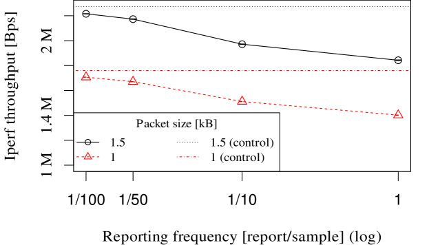
Figure 3: Mean achievable Iperf rate over 802.11g depending on the reporting rate of OML on the same medium (error bars show the standard deviation, but are barely visible with due to the $y$-axis scale in used).

4 Discussion

In this section, we discuss some of the findings from the previous result analysis and offer some recommendations on the use of OML and the instrumentation and measurement collection in networking experiments.

4.1 On OML’s Observer Effect

As mentioned earlier in Section 2.1, our main objective was to characterise the impact of OML on two types of tools widely used in the networking community, a network probing tool (Iperf) and a packet capture library (libtrace).

As a reminder, we defined in Section 2.3 our study’s two null hypotheses as follows: “the OML instrumentation of Iperf has no significant effect on its packet-sending rate nor on the accuracy of its throughput and jitter reports” and “the OML instrumentation of libtrace has no significant effect on the accuracy of its packet and timestamp reports.”

In the case of the Iperf’s instrumentation, the results from Section 3.2 show that the OML-instrumentation of the legacy reporting mode of Iperf (treatment o) does not introduce any significant deviation from the normal behaviour, at any rate. However the advanced per packet reporting mode (O) is a more intrusive and does introduce a negative bias in the reported metrics and the general behaviour of the application when used without care. The introduction in OML’s reporting loop of aggregating functions such as a sum filter (Of) completely alleviates the issue.

For the libtrace instrumentation, the results from Section 3.3 show a similar trend, where per-packets reports at very high rates have significant differences from what would be measured without OML. Once again, the proper use of upstream processing filters can cancel out this problem. Moreover in this case, we found a statistically significant positive bias introduced by the use of filters, as it allowed the packet-capturing tool to resume reading the capture buffer faster, while OML was processing the samples in a separate thread.

In a similar manner, in the context of a wireless experimentation without the availability of a separate communication channel to stream measurements, OML significantly disturbs the experiments when it is configured to capture and report every packet information. This behaviour was expected but our experiments show that the upstream processing allows to asymptotically approach the performance obtained when a dedicate reporting channel was available. These results demonstrate one of the advantage of the OML filtering capabilities and we can envision that this library would be a good candidate in the context of wireless experimentations.

Whilst the experiments presented in this study focused on the OML effect on the instrumented measurement tools, it would be legitimate to also question the effect of this library on the physical resources themselves. In order to evaluate this effect, we performed a pilot study [18] and found no significant impact on neither the CPU nor the memory usage when both applications were reporting with OML. For the sake of space and clarity, we opted not to include these results in the present document.

It is worth noting that, on the less powerful machines we used in that first study, we also found a positive significant impact of OML when used with thread-less versions of Iperf. In these cases, using OML instead of Iperf’s normal report channels would bring the performance of the non-threaded flavours to that of the threaded ones. We direct the reader to [18] for details.

Next, we propose a set of recommendations for the proper instrumentation and control network. Nevertheless, we measure the pick traffic between the receiver and the usage of OML applications.

4.2 Recommendations

OML is a good candidate for the instrumentation of distributed wireless systems. Indeed, it unifies the collection of measurements from multiple distributed nodes, and simplifies the development of measurement application (e.g., it removes the need for a complex threaded reporting system within the application). Our analyses suggest that significant impacts of OML can be avoided with adequate experimental and instrumentation design. We believe that these considerations are not specific to OML and can be applied to a larger group of instrumentation frameworks, and we further discuss them below.

First, a developer should carefully select the metrics to report together in a single MP when instrumenting either an existing or new piece of software. It is a trade-off between providing flexibility to the future user (i.e., the experimenter) and limiting the volume of information that may be reported to the collection servers. For example, in some cases it may be relevant to report all possible metrics for events always arriving at the same time (e.g., metrics about every incoming packets), whereas in other cases only some aggregate metrics may be of interests (e.g., throughput or jitter).

This point highlights the decoupling of instrumentation concerns from measurement ones, which we believe is a desirable feature of an instrumentation framework. This allows the person in charge of instrumenting an application to expose as many measurement points as possible without any assumptions on the experiments which will use it. Thus, the experimenters retain the latitude of selecting only the relevant MPs for their study, without having to tinker with the application’s code any further. Only the selected MPs would then generate measurements. Such decoupling enables the reuse of instrumented applications in various types of studies, and gives the experimenters the final choice on what data to collect. As a simple example, a researcher working on wireless MAC protocol could enable only the radiotap MP when using our OML-instrumented trace-oml2  while another researcher working on an application protocol and using the same tool could enable only the udp MP.

An experimenter would also have to ensure that the volume of measurements to collect is within the capacity of the collection server. Several solutions exist to do so, such as enabling only the relevant MPs or choosing an adequate sampling rate. In this study we analysed another solution based on the use of OML filters to pre-process data on the client side and thus reduce the number of samples. While our previous results only showed the benefits of using a sum filter over a period of time to control the volume of collected data, we believe that other kinds of filters could have similar effects. Using filters however assumes that the experimenters have an a priori idea of which metrics may be relevant to their study. It might therefore not be suitable in the exploratory phase of a study. In this case, selectively distributing the MSs between multiple collection servers would help control the load on the collection infrastructure.

Another point for the experimenter to consider is the cost of sampling. Indeed, while computing, storage, and network resources are often considered inexpensive, collecting all available raw measurements in anything than a simple experiments very often have a real cost in future data analysis and management. For example, a lot of a researcher’s time may be spent in sorting or selecting relevant data from a large measurement set, while selective sampling, perhaps motivated by a prior small-scale pilot study, may have produced more concise and relevant measurement sets. The use of filters allows this by letting the experimenters aggregate samples at different resolutions, thus giving them a fine control on the trade-off between the amount and relevance of collected data.

5 Related Work

Studies based on experimental measurements form a large part of the research in networking. Many of these studies suffer from errors related to the measurement tools or frameworks being used [20, 15]. This may be in part due to the fact that not all used instrumentation solutions have been systematically evaluated for their impact on the system under study. Even though, examples of such thorough observer effect studies exist [6, 4].

Several solutions exist to instrument and collect information from networking applications and devices, such as SNMP [12] or DTrace [5]. Similar to OML, they both allow the instrumentation of any software and/or devices. In addition, DTrace can dynamically instrument live applications, and is shipped by default with some operating systems. However, its measurement processing is limited to aggregating functions, and it does not support the streaming of measurements from different devices to a remote collection point. SNMP has been widely adopted for the management and monitoring of devices, and allows the collection of information over the network. However, it has some performance and scaling limitations when measurements from large number of devices are required within a short time window [27].

IPFIX [7] is an IETF standard, which defines a protocol for streaming information about IP traffic over the network. Similar to OML clients, IPFIX exporters stream collected and potentially filtered measurements to collector points. However, IPFIX is limited to measurements about IP flows. OML currently provides the choice of two protocols to stream measurements, a text- based and a binary one, and has the support for the IPFIX protocol on its development roadmap.

The networking community has been developing and using several measurement tools, from high performance or versatile devices such as DAG or NetFPGA [10] to specialised or distributed software such as Radiotap or DIMES [24]. Most of these tools could be instrumented with OML, i.e., as a streaming and collection framework for the data that they produce. This would allow the tools’ users to benefit from features such as filtering close to the source, easy correlation of data from many sources through the timestamped collection at one or many points, or support for temporary disconnection (e.g., DIMES agents on laptops).

6 Conclusion

In this article, we characterised the observer effect induced by instrumentation framework on measurement tools commonly used in networking research. In that regard, we proposed a methodology, based on a few easy steps and the use of analysis of variance techniques, to quantify and compare the deviations between the original tools and their instrumented counterparts. This methodology can be applied to any measurement frameworks.

In our case, we applied this methodology to analyse the differences in performance and accuracy of reported metrics. Our results showed that, though some significant negative impacts due to the OML-instrumentation could be found, proper setup of the collection system could entirely prevent them. Moreover, we identified some statistically significant positive effects, when using the in-stream filtering capabilities of OML, in some cases where the instrumented application did not use threads. Indeed, OML removes the complexity of reporting from an application, thus facilitating its development and providing users with a non-intrusive way to collect metrics from applications which main purpose is not necessary measurement. We also identified some limitations in the current OML collection server.

Finally, we presented some recommendations for developers to instrument their software, and for experimenters to configure the measurement collection from these software to avoid impacting their performance.

References

- [1] Shane Alcock, Perry Lorier and Richard Nelson “Libtrace: A Packet Capture and Analysis Library” In SIGCOMM Computer Communicatin Review 42.2 ACM, 2012 DOI: 10.1145/2185376.2185382
- [2] Marti J. Anderson “A New Method for Non-Parametric Multivariate Analysis of Variance” In Austral Ecology 26.1 Wiley-Blackwell, 2001 DOI: 10.1111/j.1442-9993.2001.01070.pp.x
- [3] Athanassios Boulis, Rodney Berriman, Saeed Attar and Yuri Tselishchev “A Wireless Sensor Network Test-bed for Structural Health Monitoring of Bridges” In LCN 2011 IEEE Computer Society, 2011 IEEE Computer Society DOI: 10.1109/LCN.2011.6115160
- [4] Lothar Braun, Alexander Didebulidze, Nils Kammenhuber and Georg Carle “Comparing and Improving Current Packet Capturing Solutions Based on Commodity Hardware” In IMC 2010 ACM, 2010 DOI: 10.1145/1879141.1879168
- [5] Bryan M. Cantrill, Michael W. Shapiro and Adam H. Leventhal “Dynamic Instrumentation of Production Systems” In USENIX 2004 USENIX Association, 2004 URL: http://www.usenix.org/event/usenix04/tech/general/full_papers/cantrill/cantrill_html/
- [6] Baek Y. Choi and Supratik Bhattacharyya “Observations on Cisco sampled NetFlow” In LSNI 2005, First ACM SIGMETRICS Workshop on Large Scale Network Inference 33.3 ACM, 2005 DOI: 10.1145/1111572.1111579
- [7] Benoit Claise et al. “Specification of the IP Flow Information Export (IPFIX) Protocol for the Exchange of IP Traffic Flow Information” RFC Editor, Internet Requests for Comment, 2008 URL: http://www.rfc-editor.org/rfc/rfc5101.txt
- [8] Carlo Demichelis and Philip Chimento “IP Packet Delay Variation Metric for IP Performance Metrics (IPPM)”, Internet Requests for Comments, 2002 URL: http://www.rfc-editor.org/rfc/rfc3393.txt
- [9] Mark Gates, Ajay Tirumala, Jon Dugan and Kevin Gibbs “Iperf version 2.0.0”, Part of Iperf’s source code distribution, 2004 NLANR applications support, University of Illinois at Urbana-Champaign URL: http://iperf.sf.net
- [10] Glen Gibb et al. “NetFPGA—An Open Platform for Teaching How to Build Gigabit-Rate Network Switches and Routers” In IEEE Transactions on Education 51.3 IEEE, 2008 DOI: 10.1109/TE.2008.919664
- [11] Gene V. Glass, Percy D. Peckham and James R. Sanders “Consequences of Failure to Meet Assumptions Underlying the Fixed Effects Analyses of Variance and Covariance” In Review of Educational Research 42.3 American Educational Research Association, 1972 DOI: 10.2307/1169991
- [12] David Harrington, Randy Presuhn and Bert Wijnen “An Architecture for Describing Simple Network Management Protocol (SNMP) Management Frameworks” RFC Editor, Internet Requests for Comment, 2002 URL: http://www.rfc-editor.org/rfc/rfc3411.txt
- [13] Michael R. Harwell, Elaine N. Rubinstein, William S. Hayes and Corley C. Olds “Summarizing Monte Carlo Results in Methodological Research: The One- and Two-Factor Fixed Effects ANOVA Cases” In Journal of Educational and Behavioral Statistics 17.4 American Educational Research Association, 1992 DOI: 10.3102/10769986017004315
- [14] Guillaume Jourjon, Thierry Rakotoarivelo and Max Ott “A Portal to Support Rigorous Experimental Methodology in Networking Research” In TridentCom 2011 Springer-Verlag Berlin, 2011 ICST URL: http://www.nicta.com.au/research/research_publications/show?id=4442
- [15] Balachander Krishnamurthy, Walter Willinger, Phillipa Gill and Martin Arlitt “A Socratic Method for Validation of Measurement-Based Networking Research” In Computer Communications 34.1 Elsevier, 2011 DOI: 10.1016/j.comcom.2010.09.014
- [16] Jean-Yves Le Boudec “Performance Evaluation of Computer and Communication Systems” EPFL Press, 2010 URL: http://perfeval.epfl.ch/lectureNotes.htm
- [17] Suhas Mathur et al. “ParkNet: Drive-by Sensing of Road-side Parking Statistics” In MobiSys 2010 ACM, 2010 DOI: 10.1145/1814433.1814448
- [18] Olivier Mehani et al. “Characterisation of the Effect of a Measurement Library on the Performance of Instrumented Tools”, Submitted to IMC 2011, 2011 URL: http://www.nicta.com.au/research/research_publications/show?id=4879
- [19] Stephen Morley and Malcolm Adams “Some Simple Statistical Tests for Exploring Single-case Time-series Data” In British Journal of Clinical Psychology 28.1 British Psychological Society, 1989 URL: http://view.ncbi.nlm.nih.gov/pubmed/2924023
- [20] Vern Paxson “Strategies for Sound Internet Measurement” In IMC 2004 ACM, 2004 DOI: 10.1145/1028788.1028824
- [21] Thierry Rakotoarivelo, Maximilian Ott, Guillaume Jourjon and Ivan Seskar “OMF: A Control and Management Framework for Networking Nestbeds” In SIGOPS Operating Systems Review 43.4 ACM, 2010 DOI: 10.1145/1713254.1713267
- [22] Dipankar Raychaudhuri et al. “Overview of the ORBIT Radio Grid Testbed for Evaluation of Next-Generation Wireless Network Protocols” In WCNC 2005 3 IEEE, 2005 DOI: 10.1109/WCNC.2005.1424763
- [23] Henning Schulzrinne, Stephen L. Casner, Ron Frederick and Van Jacobson “RTP: A Transport Protocol for Real-Time Applications” RFC Editor, Internet Requests for Comments, 1996 URL: http://www.rfc-editor.org/rfc/rfc1889.txt
- [24] Yuval Shavitt and Eran Shir “DIMES: Let the Internet Measure Itself” In SIGCOMM Computer Communucation Review 35.5 ACM, 2005 DOI: 10.1145/1096536.1096546
- [25] Darryl Veitch, Julien Ridoux and Satish B. Korada “Robust Synchronization of Absolute and Difference Clocks over Networks” In IEEE/ACM Transactions on Networking 17.2 IEEE Press, 2009 DOI: 10.1109/TNET.2008.926505
- [26] Jolyon White, Guillaume Jourjon, Thierry Rakotoarivelo and Max Ott “Measurement Architectures for Network Experiments with Disconnected Mobile Nodes” In TridentCom 2010 Springer-Verlag Berlin, 2010 ICST URL: http://www.nicta.com.au/research/research_publications/show?id=3298
- [27] Qi Zhao, Zihui Ge, Jia Wang and Jun Xu “Robust Traffic Matrix Estimation with Imperfect Information: Making Use of Multiple Data Sources” In SIGMETRICS 2006, Proceedings of the joint International Conference on Measurement and Modeling of Computer Systems 34.1 ACM, 2006 DOI: 10.1145/1140103.1140294