Weak correlation effects in the Ising model on triangular-tiled hyperbolic lattices

Abstract

The Ising model is studied on a series of hyperbolic two-dimensional lattices which are formed by tessellation of triangles on negatively curved surfaces. In order to treat the hyperbolic lattices, we propose a generalization of the corner transfer matrix renormalization group method using a recursive construction of asymmetric transfer matrices. Studying the phase transition, the mean-field universality is captured by means of a precise analysis of thermodynamic functions. The correlation functions and the density matrix spectra always decay exponentially even at the transition point, whereas power law behavior characterizes criticality on the Euclidean flat geometry. We confirm the absence of a finite correlation length in the limit of infinite negative Gaussian curvature.

I Introduction

An increasing interest in the thermodynamic behavior of various physical models on non-Euclidean (curved) surfaces has been persisting for about two decades, due to recent experimental fabrication of soft materials with conical geometry cn and magnetic nanostructures which exhibit negatively curved geometries experiment1 ; experiment2 ; experiment3 . Curved geometries are also relevant in the theory of quantum gravity q-gravity1 ; q-gravity2 . In this context, several statistical models have been investigated on simple negatively curved geometries, such as the Ising model Shima ; hctmrg-Ising-5-4 ; Sakaniwa , the $q$-state clock models hctmrg-clock-5-4 ; Baek-clock , and the XY-model XY-model .

A typical example of the negatively curved geometry is represented by the two-dimensional discretized hyperbolic surface (lattice) which is characterized by a constant negative Gaussian curvature. Among the varieties of lattice surfaces, we choose, for simplicity, a group of regular lattices that are constructed as tiling of congruent polygons of the $p$-th order with the coordination number $q$. On the hyperbolic $(p,q)$ lattices, the relation $(p-2)(q-2)>4$ is satisfied, in contrast to the relation $(p-2)(q-2)=4$ on the Euclidean flat geometry. Figure 1 shows two examples, the $(3,7)$ and $(3,13)$ lattices where the whole lattice is mapped onto the Poincaré disk Poincare .

In general, the number of the lattice sites within a certain area increases exponentially with its diameter on such hyperbolic lattices. This exponential increase limits efficiency of numerical studies of statistical models, such as the Ising model on the $(p,q)$ lattice. In particular, applications of Monte Carlo simulation face difficulties in the scaling analysis around the phase transition. Also transfer matrix diagonalization can not easily be applied due to the non-triviality in the construction of the row-to-row transfer matrices.

Despite these difficulties, one can evaluate the partition function by means of Baxter’s corner transfer matrix formalism Baxter even for the hyperbolic $(p,q)$ lattices. In this article, we use a flexible numerical implementation of Baxter’s method, so-called the Corner Transfer Matrix Renormalization Group (CTMRG) algorithm, which has been used as a tool in the computation of the partition function for (flat) two- and three-dimensional classical spin systems ctmrg-tn ; ctmrg-snapshot ; tpva-Potts . In our previous reports hctmrg-Ising-5-4 ; hctmrg-Ising-p-4 ; hctmrg-clock-5-4 ; hctmrg-J1J2 we considered the hyperbolic $(p,q)$ lattices, typically for the case with $q=4$, where the whole lattice can be divided into four quadrants, the ‘corners’. For the Ising model on the $(p,4)$ lattices, the mean-field universality was found Shima ; hctmrg-Ising-5-4 .

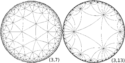
Figure 1: Poincaré disk representation of the hyperbolic lattices created by triangular tessellation $p=3$ with the coordination numbers $q=7$ (left) and $q=13$ (right).

The hyperbolic $(p,q)$ lattice with an arbitrary coordination number $q$ other than four has not been addressed by use of the CTMRG method yet. For this case the numerical renormalization procedure of the corner transfer matrices requires a technical extension upon the established numerical procedure for the $(p,4)$ lattices. In this article we introduce a new procedure which is valid for general values of $q$ and find the thermodynamic properties of the Ising model on a wider class of the $(p,q)$ lattices. In particular, the triangular tessellation ($p=3$) and the coordination number $q\geq 6$ are investigated as representative examples.

This article is organized as follows. In Sec. II we define the Ising model on the $(p,q)$ lattices. In Sec. III the recurrent renormalization algorithm of the CTMRG method is introduced. The application of CTMRG to the $(3,q)$ lattices is explained starting from $q=6$ and increasing $q$. Numerical results on the spontaneous magnetization and energy are presented in Sec. IV, with a detailed analysis of the $q$-dependence of the phase transition temperature and the corresponding scaling exponents. In Sec. V the quantum entropy and the scaling behavior of the correlation functions are observed. We also analyze the effects of the Gaussian curvature on the correlation length. We summarize the result in the last section.

II The lattice model

Consider the Ising model with the Hamiltonian

$${\cal H}(\sigma)=-J\sum\limits_{\{i,j\}}\sigma_{i}\sigma_{j}-h\sum\limits_{\{i\}}\sigma_{i}$$ (1)

defined on the hyperbolic $(p,q)$ lattices. We here use the standard notation $(p,q)$ where the first integer $p$ corresponds to the regular polygons with $p$ sides (or vertices) and where the second one $q$ stands for the coordination number which is the number of polygons meeting in each vertex. Throughout this article we focus on the triangular tiling on the $(3,q)$ lattices only. The Ising spin variables $\sigma_{i}^{~{}}=\uparrow{\rm or}\downarrow$ are located on the vertices. The first term in ${\cal H}(\sigma)$ represents the ferromagnetic coupling ($J>0$) between the nearest-neighboring Ising spins $\sigma_{i}^{~{}}$ and $\sigma_{j}^{~{}}$, and the second represents the effect of the external magnetic field $h$. Then, the partition function

$${\cal Z}=\sum\limits_{\{\sigma\}}\exp\left[-\frac{\cal H(\sigma)}{k_{\rm B}T}\right]$$ (2)

is given by the sum of the Boltzmann weights over all spin configurations which are denoted by $\{\sigma\}$. Here, $k_{\rm B}$ and $T$, respectively, are the Boltzmann constant and the temperature.

On any ($p,q$) lattice, the Boltzmann weight of the whole system can be represented as the product of the local Boltzmann weights attributed to the particular $p$-gons. In this study we define the local Boltzmann weights which are consistent with the triangular tessellation ($p=3$). For a reason we explain in the following, each local Boltzmann weight ${\cal W}_{\rm B}$ is constructed by a pair of adjacent triangles $\sigma_{a}\sigma_{b}\sigma_{d}$ and $\sigma_{b}\sigma_{c}\sigma_{d}$ as shown in Fig. 2. The local Boltzmann weight ${\cal W}_{\rm B}$ for this pair of the triangles is then given by

$${\cal W}_{\rm B}(\sigma_{a}\sigma_{b}\sigma_{c}\sigma_{d})=\exp\bigg{[}\frac{J}{2k_{\rm B}T}(\sigma_{a}\sigma_{b}+\sigma_{b}\sigma_{c}+\sigma_{c}\sigma_{d}$$

$$+\sigma_{d}\sigma_{a}+2\sigma_{b}\sigma_{d})+\frac{h}{qk_{\rm B}T}(\sigma_{a}+2\sigma_{b}+\sigma_{c}+2\sigma_{d})\bigg{]}\ .$$ (3)

The factor $2$ of $2\sigma_{b}\sigma_{d}$ arises from the fact that $\sigma_{b}$ and $\sigma_{c}$ are shared by two triangles, under the tessellation of ”bi-triangular” Boltzmann weights. Also the factor $2$ appears in $2\sigma_{b}$ and $2\sigma_{d}$ since the effect of external magnetic field $h$ should be counted for both upper and lower triangles. Under these factorizations, we proceed the calculation by the CTMRG method ctmrg-tn ; hctmrg-Ising-5-4 .

The standard numerical formalism based on the diagonalization of the row-to-row transfer matrix is not easily applied under hyperbolic geometries. It has been shown that the CTMRG method works as an alternative hctmrg-Ising-p-4 when the $(p,4)$ lattice is considered under the condition $p\geq 4$. Recall that the $(p,4)$ lattice can be divided into four equivalent quadrants by two perpendicular geodesics, and it is easily understood that each quadrant corresponds to the corner transfer matrix hctmrg-Ising-5-4 ; hctmrg-Ising-p-4 . Such division of the whole system is not generally admissible for the $(3,q)$ lattices, which is under our interest, in particular, when $q$ is odd; we tackle this case in the following.

III Recurrent RG scheme

Let us consider the generalization of the CTMRG method to the $(3,q)$ lattice with $q\geq 6$. The Boltzmann weight of the whole $(3,q)$ lattice can be represented by the product of the $q$ identical corner transfer matrices ${\cal C}_{q}^{~{}}$ surrounding the central spin $\sigma$. In this picture we can express the partition function in the product form

$${\cal Z}_{(p,q)}=\sum\limits_{\sigma}\sum\limits_{\xi_{1},\xi_{2},\dots,\xi_{q}}\prod\limits_{j=1}^{q}{\cal C}_{q}(\sigma\xi_{j}\xi_{j+1}),$$ (4)

where $\xi_{j}$ and $\xi_{j+1}$, which appear as the parameters of the corner transfer matrix ${\cal C}_{q}(\sigma\xi_{j}\xi_{j+1})$, are the block spin variables corresponding to chains of the spins from the central spin $\sigma$ towards the system boundary. We have assumed the cyclic order around $\sigma$, and thus $\xi_{q+1}\equiv\xi_{1}$ is satisfied. Throughout this paper we use the counterclockwise index ordering for the spin variables included in corner transfer matrices ${\cal C}_{q}(\sigma\xi_{j}\xi_{j+1})$, starting from any one of the two-state variables from $\sigma_{a}$ to $\sigma_{d}$. Also the renormalized spin variables $\xi_{i}$ are aligned in the same ordering, as shown on the red triangles in Figs. 2, 3, and 4.

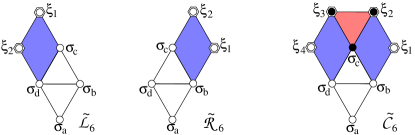
Figure 2: (Color online) Graphical representation of the extension process of the left transfer matrix ${\tilde{\cal L}}^{~{}}_{6}$, the right transfer matrix ${\tilde{\cal R}}^{~{}}_{6}$, and the corner transfer matrix ${\tilde{\cal C}}^{~{}}_{6}$ on the $(3,6)$ lattice which are defined by Eqs. (5)–(7). The filled symbols correspond to the variables which have to be summed up. The two-state and multi-state variables, respectively, are denoted by $\sigma$ and $\xi$.

Let us explain the recursive construction of the corner transfer matrix ${\cal C}_{q}(\sigma\xi_{j}\xi_{j+1})$ with respect to the successive area expansion of the whole system hctmrg-Ising-5-4 . For a tutorial purpose, we start from the $(3,6)$ lattice where the system is on the flat surface, and treat the cases $q>6$ afterward.

In contrast to the original CTMRG formulation ctmrg-tn , it is important to introduce two different kinds of ‘half-row transfer matrices’ ${\cal L}_{q}$ and ${\cal R}_{q}$ which are used for the area expansion of the corner transfer matrix. On the $(3,6)$ lattice, the area expansions of the transfer matrices ${\cal L}_{6}$ and ${\cal R}_{6}$ are performed as

$${\tilde{\cal L}}_{6}(\sigma_{d}\sigma_{a}\sigma_{b}\sigma_{c}\xi_{1}\xi_{2})={\cal W}_{\rm B}(\sigma_{a}\sigma_{b}\sigma_{c}\sigma_{d}){\cal L}_{6}(\sigma_{d}\sigma_{c}\xi_{1}\xi_{2}),$$ (5)

$${\tilde{\cal R}}_{6}(\sigma_{c}\sigma_{d}\sigma_{a}\sigma_{b}\xi_{1}\xi_{2})={\cal W}_{\rm B}(\sigma_{a}\sigma_{b}\sigma_{c}\sigma_{d}){\cal R}_{6}(\sigma_{c}\sigma_{b}\xi_{1}\xi_{2})$$ (6)

where the position of each spin variable is graphically depicted in Fig. 2. Similarly, the corner transfer matrix ${\tilde{\cal C}}_{6}$ are expanded as

$${\tilde{\cal C}}_{6}(\sigma_{d}\sigma_{a}\sigma_{b}\xi_{1}\xi_{4})=\sum\limits_{\sigma_{c},\xi_{2},\xi_{3}}{\cal W}_{\rm B}(\sigma_{a}\sigma_{b}\sigma_{c}\sigma_{d}){\cal L}_{6}(\sigma_{d}\sigma_{c}\xi_{3}\xi_{4})$$

$$\times{\cal C}_{6}(\sigma_{c}\xi_{2}\xi_{3}){\cal R}_{6}(\sigma_{c}\sigma_{b}\xi_{1}\xi_{2})\,.$$ (7)

The recursive expansion procedure in CTMRG can be initiated by setting ${\cal L}_{6}(\sigma_{a}\sigma_{b}\sigma_{c}\sigma_{d})$ $={\cal R}_{6}(\sigma_{d}\sigma_{a}\sigma_{b}\sigma_{c})$ $={\cal W}_{\rm B}(\sigma_{a}\sigma_{b}\sigma_{c}\sigma_{d})$ and ${\cal C}_{6}(\sigma_{a}\sigma_{b}\sigma_{d})$ $=\sum_{\sigma_{c}}{\cal W}_{\rm B}(\sigma_{a}\sigma_{b}\sigma_{c}\sigma_{d})$ where the multi-spin variables $\xi$ are identical with the Ising ones $\sigma$ at the beginning. In the following, we do not write spin variables explicitly for book keeping.

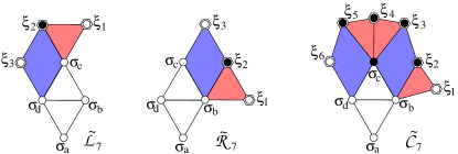
Figure 3: (Color online) The expansion process of ${\tilde{\cal L}}^{~{}}_{7}$, ${\tilde{\cal R}}^{~{}}_{7}$, and ${\tilde{\cal C}}^{~{}}_{7}$ on the ($3,7$) lattice.

We now generalize the above-mentioned expansion process for the $(3,q)$ lattices, when $q\geq 7$, where the hyperbolic surface geometry is realized. Drawing the lattice, such as shown in Fig. 1, and analyzing the inner structure of the corners, one can derive a set of recursive relations. The $q$-dependent corner transfer matrix

$${\tilde{\cal C}}^{~{}}_{q}=\sum\limits_{\sigma_{c},\xi{\rm{}^{\prime}s}}{\cal W}_{\rm B}{\cal L}^{~{}}_{q}{\cal C}^{~{}}_{q}{\cal R}^{~{}}_{q}$$ (8)

is a slight modification of Eq. (7). The relation is graphically shown in Figs. 3 and 4 for the two representative cases. Similarly, for the ‘half-row transfer matrices’, we obtain

$${\tilde{\cal L}}_{q}=\sum\limits_{\xi{\rm{}^{\prime}s}}{\cal W}_{\rm B}{\cal C}^{n_{q}}_{q}{\cal L}^{~{}}_{q}{\cal C}^{n_{q}}_{q},$$ (9)

$${\tilde{\cal R}}_{q}=\sum\limits_{\xi{\rm{}^{\prime}s}}{\cal W}_{\rm B}{\cal C}^{n_{q}}_{q}{\cal R}^{~{}}_{q}{\cal C}^{n_{q}}_{q}$$ (10)

where $n_{q}$ is the multiplicity of ${\cal C}^{~{}}_{q}$ given by

$$n_{q}=\left\lfloor\frac{q-6}{2}\right\rfloor\equiv\max\left\{n\in\mathbb{Z}\ |\ n\leq\frac{q-6}{2}\right\}.$$ (11)

In contrast to Eqs. 5 and 6, the corner transfer matrices appear in the expansion process of ${\cal L}_{q}$ and ${\cal R}_{q}$ when $q\geq 7$. The extended transfer matrices ${\tilde{\cal L}}^{~{}}_{q}$, ${\tilde{\cal R}}^{~{}}_{q}$, and ${\tilde{\cal C}}^{~{}}_{q}$ re-enter the right hand sides of Eqs. (8)-(10).

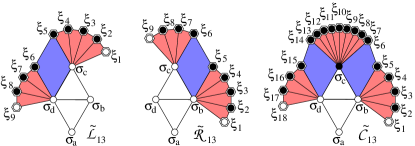
Figure 4: (Color online) The expansion process of ${\tilde{\cal L}}^{~{}}_{13}$, ${\tilde{\cal R}}^{~{}}_{13}$, and ${\tilde{\cal C}}^{~{}}_{13}$ for the ($3,13$) geometry.

The expansion process successively increases the system size by expanding the matrix dimensions of ${\tilde{\cal L}}^{~{}}_{q}$, ${\tilde{\cal R}}^{~{}}_{q}$, and ${\tilde{\cal C}}^{~{}}_{q}$. To prevent the exponential grow of computational effort, we introduce the density-matrix renormalization scheme ctmrg-tn ; hctmrg-Ising-5-4 . Let us express the block-spin transformation by the matrix $U_{\rm RG}$. The transfer matrices are ‘compressed’ by the RG transformation

$$\left(U^{\dagger}_{\rm RG}{\tilde{\cal L}}_{q}U^{~{}}_{\rm RG}\right)/{||U^{\dagger}_{\rm RG}{\tilde{\cal L}}_{q}U^{~{}}_{\rm RG}||}_{2} \to {\cal L}_{q},$$

$$\left(U^{\dagger}_{\rm RG}{\tilde{\cal R}}_{q}U^{~{}}_{\rm RG}\right)/{||U^{\dagger}_{\rm RG}{\tilde{\cal R}}_{q}U^{~{}}_{\rm RG}||}_{2} \to {\cal R}_{q},$$ (12)

$$\left(U^{\dagger}_{\rm RG}{\tilde{\cal C}}_{q}U^{~{}}_{\rm RG}\right)/{||U^{\dagger}_{\rm RG}{\tilde{\cal C}}_{q}U^{~{}}_{\rm RG}||}_{2} \to {\cal C}_{q}\,.$$

We introduced the normalization factor ${||\cdot||}_{2}$ in order to avoid the numerical over-flow in the expression of the partition function.

The central issue concerns the definition of the RG transformation. In the density-matrix renormalization scheme, $U_{\rm RG}$ is created by diagonalization of the reduced density matrix $\rho$ which may be represented in a non-Hermitian (asymmetric) form

$$\rho={\rm Tr}_{\rm env}|\psi\rangle\langle\phi|\,.$$ (13)

The trace is taken over the spin variables belonging to the environment as proposed by DMRG ctmrg-tn ; white . The states $|\psi\rangle$ and $|\phi\rangle$ correspond to two parts of the whole lattice. The Boltzmann weight for these two parts can be calculated as the product of the corner transfer matrices

$$\psi(\sigma\xi_{\alpha}\xi_{\beta}) = \sum\limits_{\xi_{1}\xi_{2},\dots,\xi_{k}}{\cal C}(\sigma\xi_{\alpha}\xi_{1}){\cal C}(\sigma\xi_{1}\xi_{2})\cdots{\cal C}(\sigma\xi_{k}\xi_{\beta}),$$ (14)

$$\phi(\mu\xi_{\gamma}\xi_{\delta}) = \sum\limits_{\xi_{1}\xi_{2},\dots,\xi_{\ell}}{\cal C}(\mu\xi_{\gamma}\xi_{1}){\cal C}(\mu\xi_{1}\xi_{2})\cdots{\cal C}(\mu\xi_{\ell}\xi_{\delta})\,,$$ (15)

where we introduced the condition $k+\ell+2=q$. The most optimal choice is to consider $k=n_{q+5}$ and $\ell=n_{q+4}$ with $n_{q}$ given by Eq. (11). We have used letter $\mu$ for the 2-state variable of $\phi$ just for distinction from $\sigma$ of $\psi$, and this choice is convenient when we construct the reduced density matrix. The normalized partition function can be written as ${\cal Z}_{(3,q)}=\langle\psi|\phi\rangle$. As an example, we obtain $k=3$ and $\ell=2$ for the $(3,7)$ lattice with the corresponding Boltzmann weights

$$\psi(\sigma\xi_{\alpha}\xi_{\beta}) = \sum_{\xi_{1}\xi_{2}\xi_{3}}{\cal C}(\sigma\xi_{\alpha}\xi_{1}){\cal C}(\sigma\xi_{1}\xi_{2}){\cal C}(\sigma\xi_{2}\xi_{3}){\cal C}(\sigma\xi_{3}\xi_{\beta})\,,$$

$$\phi(\mu\xi_{\gamma}\xi_{\delta}) = \sum_{\xi_{1}\xi_{2}}{\cal C}(\mu\xi_{\gamma}\xi_{1}){\cal C}(\mu\xi_{1}\xi_{2}){\cal C}(\mu\xi_{2}\xi_{\delta})\,.$$ (16)

Notice that if $q$ is even, $k=\ell=\frac{q}{2}-1$ resulting in $|\psi\rangle\equiv|\phi\rangle$. For this choice the reduced density matrix $\rho$ is always Hermitian (symmetric). However, for any odd $q$, $\rho$ becomes non-Hermitian (asymmetric). This may lead to severe numerical instabilities. In order to avoid them, we symmetrize the reduced density matrix. We, therefore, consider an equally weighted reduced density matrix

$$\rho(\sigma\xi_{\alpha}|\mu\xi_{\beta})=\frac{1}{2} \sum\limits_{\xi_{\gamma}} \psi^{\dagger}(\sigma\xi_{\alpha}\xi_{\gamma})\phi(\mu\xi_{\beta}\xi_{\gamma})$$ (17)

$$+ \phi^{\dagger}(\sigma\xi_{\alpha}\xi_{\gamma})\psi(\mu\xi_{\beta}\xi_{\gamma})\,.$$

Having tested both formulations of the reduced density matrix, Eqs. (13) as well as (17), we encountered numerical instabilities for the non-Hermitian case only, especially in the vicinity of the phase transition. Otherwise, both density matrix formulations yield the identical thermodynamic properties.

IV Magnetization and Energy

Since the detailed analysis of the phase transitions deep inside the hyperbolic lattice is of our interest, we concentrate on the bulk properties of a sufficiently large inner region of the lattice Sakaniwa ; hctmrg-Ising-p-4 although the influence of the system boundary is not negligible at all for the discussion of the thermodynamic properties of the system. The bulk spontaneous magnetization is an example where the value can be calculated by

$$M={\rm Tr}\left(\sigma\rho\right)/{\rm Tr}\,\rho$$ (18)

in the CTMRG formulation. Without loss of generality, we set the coupling constant $J$ and the Boltzmann constant $k_{\rm B}$ to unity, and all thermodynamic functions are evaluated in the unit of $k_{\rm B}$.

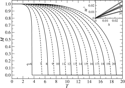
Figure 5: Spontaneous magnetizations $M$ with respect to temperature $T$ for $6\leq q\leq 20$. The inset shows the linear behavior of the cubic power of the induced magnetization $M^{3}_{~{}}$ with respect the magnetic field $h$ around the transition temperatures $T_{\rm pt}^{(q)}$.

We now consider one-point functions of the Ising model on the series of $(3,p)$ lattices in the thermodynamic limit. First of all, let us check the validity of our numerical procedure as explained in the previous section. We perform a test calculation for the flat $(3,6)$ lattice. Keeping only $m=20$ states of the multi-spin variables $\xi$ hctmrg-Ising-5-4 ; hctmrg-Ising-p-4 ; white , the obtained spontaneous magnetization is shown in Fig. 5. The estimated transition temperature $T_{\rm c}=3.641$ is quite close to the exact value $T_{\rm c}=4/\ln 3\approx 3.64096$ Baxter .

Now, we focus on the hyperbolic surfaces. In Fig. 5 we also plot the temperature dependence of the spontaneous magnetization $M$ for the coordination numbers from $7\leq q\leq 20$. The full and the dashed curves, respectively, distinguish the even and odd values of $q$. As we show later, the system is always off-critical whenever $q\geq 7$, even at the transition temperature. We, therefore, use the notation $T_{\rm pt}^{(q)}$ instead of $T_{\rm c}^{(q)}$ for $q\geq 7$; we also use $T_{\rm pt}^{(6)}$ for $q=6$ in order to unify the notation.

If a small magnetic field $h$ is applied at the transition temperature $T_{\rm pt}^{(q\geq 7)}$, the cubed induced magnetization $M^{3}_{~{}}$ is always linear around $h=0$. Thus, the model satisfies the scaling relation $M(h,T_{\rm pt})\propto h^{1/\delta}$ with the scaling exponent $\delta=3$. This value is known for the mean-field universality of the Ising model and is in full agreement with our previous results for the hyperbolic $(p\geq 5,4)$ lattices hctmrg-Ising-p-4 .

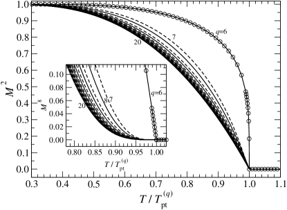
Figure 6: The squared spontaneous magnetization $M^{2}_{~{}}$ is linear with respect to the normalized temperature near the transition point. This corresponds to $\beta=\frac{1}{2}$. Inset: the linearity of the $M^{8}$ is observed only when $q=6$ where $\beta=\frac{1}{8}$.

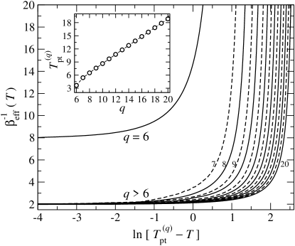
Figure 7: Convergence rate of the effective scaling exponent. Inset: scaling of the phase transition temperatures $T_{\rm pt}^{(q)}$ versus the integer $q$.

In order to observe the scaling relation of the spontaneous magnetization $M$ in a unified manner, we plot the squared magnetization $M^{2}_{~{}}$ in Fig. 6 with respect to the rescaled temperature by $T_{\rm pt}^{(q\geq 7)}$. Near the point $T=T_{\rm pt}^{(q\geq 7)}$ the mean-field behavior $M(h=0,T)\propto(T_{\rm pt}^{(q)}-T)^{\beta}_{~{}}$ with $\beta=\frac{1}{2}$ is detected. Note that on the $(3,6)$ lattice the exponent is $\beta=\frac{1}{8}$ as displayed in the inset. To detect the scaling exponent $\beta$ in a more precise manner, we calculate the effective exponent

$$\beta_{\rm eff}(T)=\frac{\partial\ln\left[M\left(h=0,T<T_{\rm pt}^{(q)}\right)\right]}{\partial\ln\left[T_{\rm pt}^{(q)}-T\right]}\,$$ (19)

by means of the numerical derivative. The convergence of $\beta_{\rm eff}(T)$ with respect to $T_{\rm pt}^{(q)}-T$ is shown in Fig. 7. It is apparent that the mean-field value $\beta=\frac{1}{2}$ is detected for any $q\geq 7$, whereas we confirm $\beta=\frac{1}{8}$ on the flat $(3,6)$ lattice only. The linear increase of the transition temperature $T_{\rm pt}^{(q\geq 7)}$ with respect to $q$ is shown in the inset where the linearity appears already around $q\gtrsim 8$. This agrees with an intuition where the mean-field behavior becomes dominant for large coordination numbers.

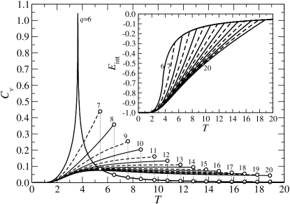
Figure 8: Specific heat as a function of temperature. The open circles connected by the vertical dotted lines show the discontinuity. Inset: temperature dependence of the internal energy.

Let us analyze the specific heat (or the heat capacity) per bond

$$C_{v}^{~{}}=\frac{\partial E_{\rm int}^{~{}}}{\partial T}$$ (20)

where $E_{\rm int}^{~{}}$ is the internal energy per bond, or equivalently, the correlation function between the two nearest-neighbor spins

$$E_{\rm int}^{~{}}=-J\langle\sigma_{i}\sigma_{i+1}\rangle=-J\,{\rm Tr}\left(\sigma_{i}\sigma_{i+1}\rho\right)$$ (21)

with $\sigma_{i}$ and $\sigma_{i+1}$ located at the center of the lattice. Figure 8 shows the results for $C_{v}^{~{}}$ and $E_{\rm int}^{~{}}$. The internal energy $E_{\rm int}^{~{}}$ is continuous for all the cases we computed. The presence of the kink in $E_{\rm int}^{~{}}$ at the transition temperature for each $q\geq 7$ corresponds to the discontinuity in $C_{v}^{~{}}$ hctmrg-Ising-p-4 ; hctmrg-J1J2 . For these cases the scaling exponent $\alpha$, which appears in the relation $C_{v}^{~{}}(h=0,T)\propto{|T_{\rm pt}^{(q)}-T|}^{-\alpha}$, is zero. It is instructive to point out that both $C_{v}^{~{}}$ and $E_{\rm int}$ in the paramagnetic region are almost independent on $q$; the tiny differences are hardly visible on the scale in the figure.

V Entropy and Correlation

Whenever the reduced density matrix $\rho$ is defined, the von Neumann (or entanglement) entropy rem1

$$S=-{\rm Tr}\left(\rho\log_{2}\rho\right)=-\sum\limits_{i}\omega_{i}^{~{}}\log_{2}\omega_{i}^{~{}}$$ (22)

can be used as a characteristic quantity which is of use for the classification of the phase transition. Figure 9 shows the temperature dependence of $S$ which remains finite for $q\geq 7$ even at the transition temperature. The entropies in the paramagnetic region are also almost independent on $q$ if $q\geq 7$ as found for $C_{v}^{~{}}$ and $E_{\rm int}$.

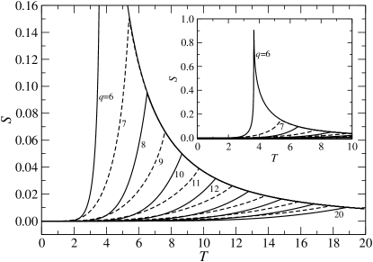
Figure 9: Temperature dependence of the von Neumann entanglement entropy. The inset displays the dominant behavior of $S$ for the $(3,6)$ lattice.

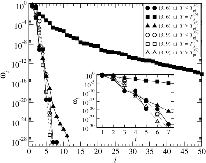
Figure 10: Decay of the density matrix spectra for the $(3,6)$ lattice (filled symbols) and the $(3,9)$ lattice (open symbols).

The decay rate of the density matrix eigenvalues $\omega_{i}^{~{}}$ is shown in Fig. 10 on a semilogarithmic scale for both $(3,6)$ and $(3,9)$ lattices. We confirm a power-law decay in $\omega_{i}^{~{}}$ only at the transition point of the $(3,6)$ lattice. Note that the eigenvalues $\omega_{i}^{~{}}$ decrease exponentially for $q\geq 7$ at the transition temperature.

The exponential decay of the density matrix spectra is also reflected in the correlation function

$$G_{i,j}={\rm Tr}\left(\sigma_{i}\sigma_{j}\rho\right)$$ (23)

between two distant sites $i$ and $j$. We place the spin $\sigma_{i}$ at the center of the system and $\sigma_{j}$ at the system boundary. Therefore, as the lattice expands its size via the recursive steps in CTMRG, the distance between these two spins increases progressively.

Figure 11 depicts $\log_{10}\left(G_{i,j}\right)$ as a function of $|i-j|$ for the $(3,6)$ lattice (open symbols) and the $(3,9)$ lattice (full symbols). It is evident that the correlation functions always decay exponentially on the $(3,9)$ lattice regardless of the temperature. We remark that an analogous exponential decay of $G_{i,j}$ has been observed for all $q\geq 7$ (not shown). On the $(3,6)$ lattice, the correlation function decays as a power law at the transition temperature, as seen in the inset.

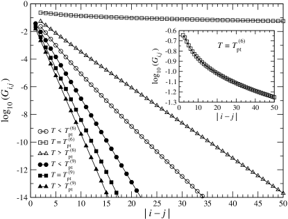
Figure 11: Decay of the correlation functions with respect to the distance $|i-j|$. The open and the full symbols, respectively, correspond to the $(3,6)$ lattice calculated at $T=3.0$, $3.641$, and $5.0$, and the $(3,9)$ lattice at $T=6.0$, $7.608$, and $9.0$.

In the following, we compare the Gaussian curvature associated to the $(3,q)$ lattice with the correlation length at the transition temperature. There are several ways to define the correlation length $\xi_{q}$ Baxter ; Frank . For example, the decay rate of the correlation function directly provides $\xi_{q}$. This is straightforward, but the region of the distance for the fitting analysis has to be valued carefully. Another possibility consists in using the largest eigenvalue $\lambda_{0}(q)$ and the second largest one $\lambda_{1}(q)$ of the row-to-row transfer matrix where $\xi_{q}$ is determined from

$$\frac{1}{\xi_{q}}=\ln\left[\frac{\lambda_{0}(q)}{\lambda_{1}(q)}\right]\,.$$ (24)

The relation can be generalized to the $(3,q\geq 7)$ lattices, in analogy to our previous formulations for the $(5,4)$ lattice hctmrg-corrlen , via the construction of the row-to-row transfer matrix

$${\cal T}_{q}(\xi_{1}\sigma_{a}\xi_{2}|\xi_{1}^{\prime}\sigma_{a}^{\prime}\xi_{2}^{\prime})={\cal L}_{q}(\sigma_{a}^{\prime}\xi_{1}^{\prime}\xi_{1}\sigma_{a}){\cal L}_{q}(\sigma_{a}\xi_{2}\xi_{2}^{\prime}\sigma_{a}^{\prime})\,.$$ (25)

Using the notation of the recurrence scheme introduced in the previous section, we calculate $\xi_{q}$ by use of Eq. (24).

The Gaussian curvature $K_{q}$ that corresponds to $(3,q)$ lattice is given by Mosseri

$$K_{q}=\frac{1}{{(iR_{q})}^{2}}=-4\,{\rm arccosh}\left[\frac{1}{2\sin\left(\frac{\pi}{q}\right)}\right]$$ (26)

where $R_{q}$ is the curvature radius of the hyperbolic surface. Recall that $K_{q}$ must be zero on the Euclidean flat space ($q=6$). Figure 12 shows the relation between $K_{q}$ and the shifted transition temperature $T_{\rm pt}^{(q)}-T_{\rm pt}^{(6)}$. The lower-left inset shows complementary information about $R_{q}$. The correlation function $\xi_{q}$ calculated around the phase transition for three different $q$’s is plotted in the upper-right inset. Notice that $\xi_{q}$ reaches its maximum at the phase transition which is not well visible as $q$ increases.

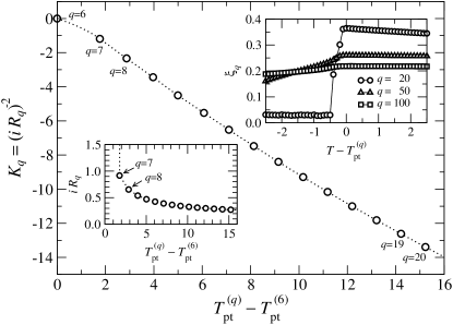
Figure 12: Gaussian curvature $K_{q}$ with respect to the shifted phase transition temperatures for $6\leq q\leq 20$. The inset on the left shows the related radius of the curvature $iR_{q}$ via Eq. (26) while that on the right shows the correlation length in the vicinity of the phase transition.

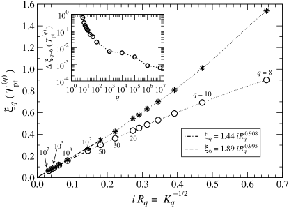
Figure 13: Asymptotic scaling of the correlation length $\xi_{q}$ at the transition temperatures $T_{\rm pt}^{(q)}$ with respect to $R_{q}$. The thin dotted lines serve as a guide to the eye. The inset shows the difference $\Delta\xi_{6-q}(T_{\rm pt}^{(q)})$ in Eq. (27) with respect to $q$ on a double logarithmic scale.

Figure 13 shows the dependence of the correlation length $\xi_{q}(T)$ at the transition temperature with respect to the curvature radius $R_{q}$. In order to collect these data, we performed extensive calculations up to 32 digits numerical precision for the value of $q$ as large as $q=10\,000\,000$ where the corresponding Gaussian curvature $K_{10^{7}}$ is approximately $900$. Note that both quantities diverge on the $(3,6)$ lattice, and therefore $\xi_{6}(T_{\rm pt}^{(6)})$ and $R_{6}$ are not shown. Let us focus on the limit $R_{q}\to 0$ which corresponds to $q\rightarrow\infty$. Evidently, the correlation length $\xi_{q}$ decreases to zero as $q$ tends toward infinity (the circles). Applying a least-square fit, we obtain the relation $\xi_{q}=1.44(iR_{q}^{~{}})^{0.908}_{~{}}$ as shown by the thick dot-dashed curve. If we consider the error in the calculation of the correlation length, we can conjecture that $\xi_{q}$ is proportional to $R_{q}$.

Recall that the specific heat $C_{v}^{~{}}$, the internal energy $E_{\rm int}$, and the entanglement entropy $S$ turned out to be weakly dependent on the value of $q$ in the paramagnetic region $T>T_{\rm pt}^{(q)}$ for $q\geq 6$. Thus, it can be conjectured that the disordered state is not modified by the presence of the negative curvature. We, therefore, compare $\xi_{q\geq 7}$ just at the transition temperature $T_{\rm pt}^{(q)}$ with the correlation length $\xi_{6}$ at the temperatures $T=T_{\rm pt}^{(q)}$. These values are plotted in Fig. 13 by the asterisks. Since $T_{\rm pt}^{(q)}$ almost linearly increases with $q$ for large values of $q$, the dotted line goes to the origin of the graph. The circles and the asterisks in Fig. 13 are of the same order for all $q$, and this fact supports our conjecture that $R_{q}$ represents the only characteristic length of the hyperbolic lattice and that the phase transition occurs at the temperature where $\xi_{q}$ is of the same order as $R_{q}$. Note that $\xi_{6}(T_{\rm pt}^{(q)})>\xi_{q}(T_{\rm pt}^{(q)})$ is always fulfilled as plotted in the inset of Fig. 13 where we show the difference

$$\Delta\xi_{6-q}(T_{\rm pt}^{(q)})=\left[\xi_{6}(T_{\rm pt}^{(q)})-\xi_{q}(T_{\rm pt}^{(q)})\right]\,.$$ (27)

The relation $\xi_{6}(T_{\rm pt}^{(q)})>\xi_{q}(T_{\rm pt}^{(q)})$ may be explained by the effect of the negative curvature that prevents from a kind of loop-back of the correlation effect. Such suppression is also expected to be present in higher-dimensional hyperbolic lattices and could be analytically studied by means of the high temperature expansion.

We conjecture the reason why the correlation length remains finite even at the phase transition temperature $T_{\rm pt}^{(q)}$ for $q>6$, as follows. First of all, the hyperbolic plane contains the typical length scale $R_{q}^{~{}}$, and it might prevent scale invariance of the state expected at the criticality. A more constructive interpretation could be obtained from the observation on the row-to-row transfer matrix. The calculation of $\xi_{q}$ by means of Eq. (24) requires diagonalization of the row-to-row transfer matrix ${\cal T}_{q}(\xi_{1}\sigma_{a}\xi_{2}|\xi_{1}^{\prime}\sigma_{a}^{\prime}\xi_{2}^{\prime})$ in Eq. (25). The matrix corresponds to an area which connects (transfers) the row of the neighboring spins $\{\xi_{1}\sigma_{a}\xi_{2}\}$ with the adjacent ones $\{\xi_{1}^{\prime}\sigma_{a}^{\prime}\xi_{2}^{\prime}\}$. The shape of this area is very different from the standard transfer matrix on the Euclidean lattice, which corresponds to a stripe of constant width. On the hyperbolic surfaces, however, this distance between the spin rows is not uniform. The distance is minimal at the center of the transfer matrix, i.e., between the two spins $\sigma_{a}$ and $\sigma_{a}^{\prime}$, and it increases exponentially with respect to the deviation from the center to the direction of spin rows. Such a geometry hctmrg-corrlen could be imagined from the recurrence construction in Eq. (9). As a consequence, the transfer matrix has an effective width, which is of the order of the curvature radius $R_{q}$. The region outside this width contributes as a sort of the boundary spins that imposes mean-field effect to the bulk part. This situation is analogous to the Bethe lattice, being interpreted here as ($\infty,q$)-lattices. hctmrg-Ising-p-4 . Thus the Ising universality could be observed only when the correlation length $\xi_{q}$ is far less than the curvature radius, $\xi_{q}\llless R_{q}$. As the length $\xi_{q}$ increases toward the transition temperature, we expect a transient behavior to the mean-field behavior around the point when $\xi_{q}$ becomes comparable to $R_{q}$. We are confirming these conjectures and the details would be reported in our subsequent work.

VI Conclusions

We have presented a detailed analysis of various non-Euclidean lattices forming surfaces with hyperbolic curvatures. In addition to our previous works on the ($p,4$) lattices, we studied the complementary situation represented by the $(3,q)$ lattices. This task required a reformulation of the existing CTMRG algorithm. We, therefore, considered the half-row transfer matrices and the corner transfer matrices including asymmetric (non-Hermitian) cases. For the lattices with odd $q$’s, we symmetrized the density matrix by the way which has been accepted by the DMRG community white .

We treated the Ising model on the $(3,q)$ lattice with coordination number $6\leq q\leq 10^{7}$. The phase transition temperatures are determined from the analysis of the magnetization, internal energy, specific heat, and the von Neumann entanglement entropy. We have shown that the transition temperature $T_{\rm pt}^{(q)}$ linearly increases with $q$ for larger values of $q$. The scaling behavior of the thermodynamic functions, including their related scaling exponents $\alpha=0$, $\beta=\frac{1}{2}$, and $\delta=3$, obeys the mean-field universality class. The mean-field nature of the hyperbolic surfaces is characterized by the exponential decay of the reduced density matrix eigenvalues and the correlation functions even at the transition temperature.

We further evaluated the radius of the Gaussian curvature $R_{q}$ for the generic ($3,q\geq 6$) lattice geometry and compare it to the results for the correlation length extracted from the row-to-row transfer matrix. We found a strongly suppressed correlation length $\xi_{q}<1$ at the transition point for any $q\geq 7$. We conjecture that $\xi_{q}$ is proportional to $R_{q}$ in the large $q$ limit.

In order to elucidate the origin of the mean-field universality induced by the hyperbolic geometry, our future studies aim at the treatment of specific hyperbolic geometries with non-constant Gaussian curvatures in order to systematically approach the Euclidean (flat) geometry.

- (1) W.A. Moura-Melo, A.R. Pereira, L.A.S. Mol, A.S.T. Pires, Phys. Lett. A 360, 472 (2007).
- (2) H. Yoshikawa, K. Hayashida, Y. Kozuka, A. Horiguchi, and K. Agawa, Appl. Phys. Lett. 85, 5287 (2004).
- (3) F. Liang, L. Guo, Q.P. Zhong, X.G. Wen, C.P. Chen, N.N. Zhang, and W.G. Chu, Appl. Phys. Lett. 89, 103105 (2006).
- (4) A. Cabot, A. P. Alivisatos, V. F. Puntes, L. Balcells, O. Iglesias, and A. Labarta, Phys. Rev. B 79, 094419 (2009).
- (5) V.A. Kazakov, Phys. Lett. A 119, 140 (1986).
- (6) C. Holm and W. Janke, Phys. Lett. B 375, 69 (1996).
- (7) H. Shima and Y. Sakaniwa, J. Phys. A 39, 4921 (2006).
- (8) Y. Sakaniwa, H. Shima, Phys. Rev. E 80, 021103 (2009).
- (9) K. Ueda, R. Krcmar, A. Gendiar, and T. Nishino, J. Phys. Soc. Jpn. 76, 084004 (2007).
- (10) A. Gendiar, R. Krcmar, K. Ueda, and T. Nishino, Phys. Rev. E 77, 041123 (2008).
- (11) S.K. Baek, P. Minnhagen, H. Shima, and B.J. Kim, Phys. Rev. E 80, 011133 (2009).
- (12) S.K. Baek, H. Shima, and B.J. Kim, Phys. Rev. E 79, 060106(R) (2009).
- (13) J.W. Anderson, Hyperbolic Geometry, second edition, Springer, 2005.
- (14) R.J. Baxter, Exactly Solved Models in Statistical Mechanics, Academic Press, London, 1982.
- (15) T. Nishino, J. Phys. Soc. Jpn. 65, 891 (1996).
- (16) K. Ueda, R. Otani, Y. Nishio, A. Gendiar, T. Nishino, J. Phys. Soc. Jpn. 74, 111 (2005).
- (17) A. Gendiar and T. Nishino, Phys. Rev. E 65, 046702 (2002).
- (18) R. Krcmar, A. Gendiar, K. Ueda, and T. Nishino, J. Phys. A 41, 125001 (2008).
- (19) R. Krcmar, T. Iharagi, A. Gendiar, and T. Nishino, Phys. Rev. E 78, 061119 (2008).
- (20) S.R. White, Phys. Rev. Lett. 69, 2863 (1992); Phys. Rev. B 48, 10345 (1993).
- (21) Strictly speaking, the non-Hermitian form of the density matrix cannot be used to evaluate the entanglement entropy due to the definition of the density matrix itself. Therefore, we always apply the symmetrized form of the density matrix for odd ’s according to Eq. (17). The entanglement entropy for odd ’s is then considered to be less reliable than for even ’s, and we regard such entropy as complementary information.
- (22) R. Mosseri and J.F. Sadoc, J. Physique - Lettres 43 L-249 (1982).
- (23) B. Pirvu, G. Vidal, F. Verstraete, L. Tagliacozzo, arXiv:1204.3934.
- (24) T. Iharagi, A. Gendiar, H. Ueda, and T. Nishino, J. Phys. Soc. Jpn. 79, 104001 (2010).