Pulsed ”three-photon” light

Abstract

Generating multi-photon entangled states is a primary task for applications of quantum information processing. We investigate production of photon-triplet in a regime of light amplification in second-order nonlinear media under action of a pulsed laser beam. For this goal the process of cascaded three-photon splitting in an optical cavity driven by a sequence of laser pulses with Gaussian time-dependent envelopes is investigated. Considering production of photon-triplet for short-time regime and in the cascaded three-wave collinear configuration we shortly analyze preparation of polarization-non-product states looking further applications of these results in the cascaded optical parametric oscillator. It is also demonststed the nonclassical characteritics of the photon-triplet in phase-space on the base of the Wigner function. Calculating the normalized third-order correlation functions below-and at the generation threshold of cascaded optical parametric oscillator, we demonstrate that in the pulsed regime, depending on the duration of pulses and the time-interval separations between them, the degree of three-photon-number correlation essentially exceed the analogous one for the case of continuous pumping.

I Introduction

Multiphoton entangled states have attracted a great interest in probing the foundations of quantum theory and constitute a powerful quantum resource with promising potential for various applications in quantum information technologies. Recently, experimental efforts in the direct production of multiphoton joint states, particularly, three- or four-photon states have paved a new stage for the study of multipartite entanglement Hamel . Indeed, the simultaneous generation of three photons is at the origin of intrinsic three-particle quantum properties such as Greenberger-Horne-Zeilinger (GHZ) -class and W-class quantum entanglement H2 - H5 . Up to now, several physical systems have been proposed for the generation of photon triplet including third-order nonlinear medium H6 and cascaded spontaneous parametric down-conversion (PDC) H7 ; H8 . Experimentally, three-photon down-conversion was studied in third-order nonlinear media H9 - H11 and also by using cascaded second-order nonlinear parametric processes Hl2 . Direct generation of photon triplets using cascaded photon-pairs has been demonstrated in periodically poled lithium niobate crystals Hamel . The distinction of three-photon GHZ and W states entangled in time and space has been also reported Hl3 ; Hl4 . It was also shown that intracavity three-photon down-conversion can be effectively realized in cascaded optical parametric oscillator (OPO) Hl5 . This scheme that involves cascading second-order nonlinearities is based on the parametric processes of splitting and summing in which the frequencies between the pump and two subharmonics frequencies are in the ratio of $3:2:1$. Experimental realization of cascaded OPO by using the dual-grid method of quasi-phase matching (QPM) has been done in Ref. Hl6 . Most recently, joint quantum states of three-photons with arbitrary spectral characteristics have been studied on the base of optical superlattises Hl7 for the cascaded configuration proposed in Hl5 . Two cascaded configurations have been considered in Hl7 that lead to production of spontaneous photon triplet in cascaded PDC and generation of high intensity mode due to cascaded three-photon splitting in optical cavity.

In this paper we continue the investigation of cascaded three-photon splitting in an optical cavity following the paper Hl7 . Our goal is twofold. In one part of the present paper we extend our previous results regarding three-photon splitting in optical cavity for an experimentally available scheme that is a cascaded parametric oscillator pumped by a sequence of Gaussian laser pulses (see, Sects. II and III). The other part of the paper is devoted to studies of quantum properties of ”three-photon” mode. We discuss preparation of non-product states that are superposition of three-photon polarization states, however, without any consideration of cavity effects (see, Sec. IV). We also calculate the Wigner function of the subharmonic, i.e. ”three-photon mode” showing the negativity in phase-space (see, Sec. V). Our analysis includes calculation of third-order correlation function of photon numbers for various operational regimes of pulsed OPO(see, Sec. VI). It is known, that it is possible to control the behavior of quantum dissipative system by a train of pulses. In this paper, we use this approach for suppression of dissipation and cavity induced feedback in cascaded OPO that leads to increasing the level of three-photon-number correlation.

II Periodically pulsed cascaded OPO: Generation threshold

In this section we briefly describe the cascaded optical parametric oscillator (OPO) with a triply resonant optical ring cavity driven by a sequence of laser pulses. The semiclassical and quantum theories of this device for the monochromatic pump field were developed in Refs. Hl5 ; Hl7 and here we only add some important details regarding cascaded OPO under laser pulses with Gaussian time-dependent envelopes. This cascaded configuration involves the fundamental mode driven by an external pump field at the central frequency $\omega_{0}$ with an amplitude $E_{L}$ and two subharmonic modes at the frequencies $\omega_{1}=\frac{\omega_{0}}{3}$ and $\omega_{2}=\frac{2\omega_{0}}{3}$. Due to intracavity parametric type-I three-wave interactions pump field is converted to the subharmonics throughout two cascaded processes: $\omega_{0}\rightarrow\omega_{1}+\omega_{2}$ and $\omega_{2}\rightarrow\omega_{1}+\omega_{1}$. Subharmonic modes have the same plane polarizations and are all propagating in the same direction. The pump field consists from the sequence of Gaussian laser pulses with the amplitude

$$E(t,z)=E_{L}f(t)e^{-i(\omega_{0}t-k_{L}z)},$$ (1)

$$f(t)=\sum_{n=0}^{\infty}e^{-(t-t_{0}-n\tau)^{2}/T^{2}},$$ (2)

where $T$ is the duration of pulses that are separated by time intervals $\tau$.

The cascaded OPO is dissipative, because the modes suffer from losses due to partially transmission of light through the mirrors of the cavity. We consider below the case of high cavity losses for the pump mode $(\gamma_{0}\gg\gamma,\gamma_{1}=\gamma_{2}=\gamma)$, when the pump mode is eliminated adiabatically in non-depletion approximation. In this case, the effective interaction Hamiltonian in the rotating wave approximation reads as

$$H_{int}=i\hbar\chi_{1}E_{0}f(t)\left(a_{1}^{+}a_{2}^{+}-a_{1}a_{2}\right)+i\hbar\chi_{2}\left(a_{1}^{+2}a_{2}-a_{1}^{2}a_{2}^{+}\right),~{}~{}~{}~{}~{}$$ (3)

where $E_{0}=E_{L}/\gamma_{0}$, $a_{i}$ (i=1,2) are the operators of the modes at the frequencies $\omega_{1}=\frac{\omega_{0}}{3}$ and $\omega_{2}=\frac{2\omega_{0}}{3}$ and the coupling constants between the modes are expressed through the Fourier spectra of the second-order susceptibilities of nonlinear crystals of the length $L$

$$\chi_{1}=\int^{L}_{0}dz\chi^{\left(2\right)}(z)e^{i\Delta k_{1}(z)z},$$ (4)

$$\chi_{2}=\int^{L}_{0}dz\chi^{\left(2\right)}(z)e^{i\Delta k_{2}(z)z}.$$ (5)

We assume collinear, one-dimensional on $z$ quasi-phase-matching with the phase mismatch vectors

$$\Delta k_{1}(z)=k_{L}(\omega_{0},z)-k_{1}(\omega_{1},z)-k_{2}(\omega_{2},z),$$ (6)

$$\Delta k_{2}(z)=k_{2}(\omega_{2},z)-2k_{1}(\omega_{1},z)$$ (7)

analyzed in the details Hl7 .

In this regime, the stochastic equations of motion for the complex c-number variables $\alpha_{1,2}$ and $\beta_{1,2}$ corresponding to the operators $a_{1,2}$ and $a_{1,2}^{+}$, have the following form

$$\frac{d\alpha_{1}}{dt}=-\gamma_{1}\alpha_{1}+E_{0}f(t)\chi_{1}\beta_{2}+2\chi_{2}\alpha_{2}\beta_{1}+W_{\alpha_{1}}(t),$$ (8)

$$\frac{d\beta_{1}}{dt}=-\gamma_{1}\beta_{1}+E_{0}f(t)\chi_{1}\alpha_{2}+2\chi_{2}\beta_{2}\alpha_{1}+W_{\beta_{1}}(t).$$ (9)

The equations for $\alpha_{2},\beta_{2}$ are obtained from (8), (9) by exchanging the subscripts $(1)\rightleftharpoons(2)$. Our derivation is based on the Ito stochastic calculus, and the nonzero stochastic correlators are:

$$\langle W_{\alpha_{1}}(t)W_{\alpha_{2}}(t^{{}^{\prime}})\rangle=\chi_{1}\frac{E_{L}f(t)}{\gamma_{0}}\delta(t-t^{{}^{\prime}}),$$ (10)

$$\langle W_{\alpha_{1}}(t)W_{\alpha_{1}}(t^{{}^{\prime}})\rangle=2\chi_{2}\alpha_{2}\delta(t-t^{{}^{\prime}}),$$ (11)

$$\langle W_{\beta_{1}}(t)W_{\beta_{1}}(t^{{}^{\prime}})\rangle=2\chi_{2}\beta_{2}\delta(t-t^{{}^{\prime}}),$$ (12)

$$\langle W_{\alpha_{2}}(t)W_{\alpha_{2}}(t^{{}^{\prime}})\rangle=2\chi_{2}\alpha_{1}\delta(t-t^{{}^{\prime}}).$$ (13)

The Eqs. (8), (9) and the correlation functions modifies the analogous ones derived for OPO with monochromatic pumping Hl5 on the case of non-stationary pump field.

In accordance with the cited paper, for the monochromatic driven cascaded OPO, zero-amplitude solutions $\alpha_{1}=\alpha_{2}=0$ of Eqs. (8), (9) with $f(t)=1$ are stable, if $E_{L}<E_{th}=\frac{\gamma_{0}}{\chi_{1}}\sqrt{\gamma_{1}\gamma_{2}}$, while steady-state photon numbers $n_{1}$ and $n_{2}$ display histeresis-cycle behavior in a small domain $\frac{2\sqrt{2}}{3}<E_{L}/E_{th}<1$. Thus, remarkable feature of OPO under monochromatic pump is comparatively low generation threshold that depends from the second-order susceptibility in comparison with the scheme of direct intracavity three-photon down-conversion, where the pump power threshold is determined by the third-order susceptibility H9 .

Below, we derive the threshold value for OPO driven by trains of Gaussian pulses. The analysis of stochastic equations shows that similar to the standard OPO with monochromatic pump field amplitude, the periodically pulsed OPO also exhibits threshold behavior, which is easily described through the period averaged pump field amplitude $\overline{f(t)}=\frac{1}{\tau}\int_{0}^{\tau}f(t)dt$. We demonstrate this statement analyzing the stability of zero-amplitude solutions of $\alpha_{1}=\alpha_{2}=0$ of Eqs. (8), (9) for both modes below threshold and for the case when the decay rates of subharmonics are equal one to the order, $\gamma_{1}=\gamma_{2}=\gamma$. To check the stability we turn to the linearized on the small deviations $\delta\alpha_{i},\delta\beta_{i}$ the equations in the semicalssical approach without noise terms. These equations can be rewriten in the following form:

$$\frac{d}{dt}\delta X_{\pm}=(-\gamma\pm\frac{E_{L}}{\gamma_{0}}\chi_{1}f(t))\delta X_{\pm},$$ (14)

$$\frac{d}{dt}\delta Y_{\pm}=(-\gamma\pm\frac{E_{L}}{\gamma_{0}}\chi_{1}f(t))\delta Y_{\pm},$$ (15)

through the quadrature field variables defined as $\delta\alpha_{\pm}=\delta\alpha_{1}\pm\delta\alpha_{2}$ and $\delta X_{\pm}=\frac{1}{2}(\delta\alpha_{\pm}+\delta\alpha^{*}_{\pm}),\delta Y_{\pm}=\frac{1}{2i}(\delta\alpha_{\pm}-\delta\alpha^{*}_{\pm})$. In these variables the time evolution has the simple form

$$\delta X_{\pm}(t)=\Lambda_{\pm}(t,t_{0})\delta X_{\pm}(t_{0}),$$ (16)

$$\delta Y_{\pm}(t)=\Lambda_{\mp}(t,t_{0})\delta Y_{\pm}(t_{0}),$$ (17)

$$\Lambda_{\pm}(t,t_{0})=exp(\pm\frac{E_{L}\chi_{1}}{\gamma_{0}}\int^{t}_{0}f(t^{{}^{\prime}})dt^{{}^{\prime}}-\gamma(t-t_{0})).$$ (18)

Analyzing semiclassical equations and operational regimes we choose the switching time in infinity, i.e. $t_{0}\rightarrow-\infty$, and add in (2) terms with negative $n$. In this case, the function $f(t)$ is periodic on time $f(t+\tau)=f(t)$ and the analysis is simplified. Since the function $f(t)$ is periodic on time, we can obtain the general formula $\int^{t}_{t_{0}}f(t)dt=\overline{f(t)}(t-t_{0})+F(t)-F(t_{0})$, where $F(t)$ is a periodic function, $F(t+\tau)=F(t)$. Therefore, we see from (16), (17), (18) that the solution $\alpha_{i}=0$ below-threshold is stable if $E_{L}<\frac{\gamma_{0}\gamma}{\chi_{1}}\overline{f(t)}$. It is easy to check also that due to noted periodicity of the amplitude the following formula takes place (see, for example HADAM )

$$\int_{0}^{\tau}dt\sum_{n=-\infty}^{\infty}e^{-(t-n\tau)^{2}/T^{2}}=\int_{-\infty}^{\infty}dte^{-t^{2}/T^{2}}.$$ (19)

This formula allows us to calculate the averaged value of the amplitude $f(t)$. On the whole, we arrive to the result that for the case of Gaussian pulses above threshold regime is realized if

$$E_{L}\geq\overline{E_{th}}=\frac{\tau}{T\sqrt{\pi}}E_{th}=\frac{\tau}{T\sqrt{\pi}}\frac{\gamma_{0}\gamma}{\chi_{1}}.$$ (20)

The important peculiarity of the system proposed is that the threshold value $\overline{E_{th}}$ depends on the coupling constant $\chi_{1}$ which is related to the second-order susceptibility as well as depends on the characteristics of laser pulses.

III Numerical simulation of dissipation and decoherence

The cascaded OPO is dissipative, because the modes suffer from losses due to partial transmission of light through the mirrors of the cavity and due to quantum fluctuations. We analyse dissipative and decoherence effects on the base of master equation for the density operator of the cavity modes in the Lindblad form

$$\frac{\partial\rho}{\partial t}=\frac{1}{i\hbar}[H_{int},\rho]+\sum_{i=1,2}{\gamma_{i}\left(2a_{i}\rho a^{+}_{i}-a^{+}_{i}a_{i}\rho-\rho a^{+}_{i}a_{i}\right)}.$$ (21)

We calculate the quantities of interest (the photon number distributions, Wigner functions, etc.) mainly for the subharmonic mode (1) by using the reduced density operator $\rho_{1}(t)$ which is constructed from the density operator $\rho(t)$ of both modes by tracing over the mode (2), $\rho_{1}(t)=Tr_{2}(\rho)$. We analyze the master equation numerically using quantum state diffusion method (QSD) H18 , claster . According to this method, the reduced density operator is calculated as the ensemble mean

$$\rho(t)=M(|\psi_{\xi}(t)\rangle\langle\psi_{\xi}(t)|)=\lim_{N\rightarrow\infty}\frac{1}{N}\sum_{\xi}^{N}|\psi_{\xi}(t)\rangle\langle\psi_{\xi}(t)|$$ (22)

over the stochastic pure states $|\psi_{\xi}(t)\rangle$ describing evolution along a quantum trajectory. The stochastic equation for the state $|\psi_{\xi}(t)\rangle$ involves Hamiltonian described by Eq. (3) and the Lindblad operators described by noise terms in the master equation (21). We calculate the density operator using an expansion of the state vector $|\psi_{\xi}\rangle$ in a truncated basis of Fock’s number states of modes of the subharmonics (1) and (2)

$$|\psi_{\xi}(t)\rangle=\sum_{n}a_{n_{1},n_{2}}^{\xi}(t)|n_{1}\rangle_{1}|n_{2}\rangle_{2}.$$ (23)

Details of analogous calculations for an anharmonic oscillator in time-modulated field can be found in H19 ). The numerical simulations are performed in the truncated Fock basis of the subharmonic modes that are limited by 500 photons. This approximation is valid for the case of strong nonlinear couplings $\chi_{1}$ and $\chi_{2}$ with respect to the dissipation parameters.

IV Production of polarization, non-product states of photon triplet in collinear configuration

Three-photon correlations allow the creation of tripartite entangled states such as the GHZ state. For cascaded SPDC in noncollinear configuration spatially-polarization GHZ states has been considered in Hl7 . Below we apply the results obtained for preparation of three-photon polarization states in collinear configuration of interacting waves. Recently, a simple but highly efficient source of polarization-entangled photon pairs at nondegenerate wavelengths and in collinear configuration has been demonstrated HAPL . We consider the production of polarization-entangled photon triplet. It is possible for the case when cascaded processes involve polarized photons.

Thus, we modify the above results considering three-wave interaction with the indexes of polarization states. Looking further applications of above results for intracavity three-photon down-conversion in collinear configuration of cascading processes we concentrate on consideration of non-product states that are entangled only on polarization degree of freedom but not on spatial variables. Thus, including into consideration the polarization states of the photons we assume that the type-II process $\omega_{0}\rightarrow\omega_{1}+\omega_{2}$ create the pair of photons with $a$ vertical $V,(a_{1}(V),(a_{2}(V))$ and horizontal $H,(a_{1}(H),(a_{2}(H))$ polarizations in collinear configuration. If the pump field is oriented at $45^{\circ}$ to the horizontal and vertical axes two processes $\omega_{0}\rightarrow\omega_{1}(V)+\omega_{2}(H)$ and $\omega_{0}\rightarrow\omega_{1}(H)+\omega_{2}(V)$ take place in the first crystal. The next process is considered as the type-I parametric process. In type-I conversion, photon pairs are created with the same polarization state, but ortogonal to the input mode. Therefore, the second, type-I crystal is arranged in the manner that the following process: $\omega_{2}(H)\rightarrow\omega_{1}(V)+\omega_{1}(V)$ and $\omega_{2}(V)\rightarrow\omega_{1}(H)+\omega_{1}(H)$ should be realized.

For simplicity, we restrict our attention considering frequency-uncorrelated three-photon states and assume that the process under photons with $(V)$ and $(H)$ polarizations are described by the equal coupling constants. Thus, we assume that photon pairs in three-wave processes : $\omega_{0}\rightarrow\omega_{1}+\omega_{2}$, $\omega_{2}\rightarrow\omega^{{}^{\prime}}_{1}+\omega^{"}_{1}$ have correlations on the polarization, but not on the spectral lines. In analogy with Eq.(3), we model the sum of the corresponding parametric interactions by the following effective Hamiltonian

$$H=H_{1}+H_{2},~{}~{}~{}~{}~{}~{}~{}~{}~{}~{}~{}~{}~{}~{}~{}~{}$$ (24)

$$H_{1}=i\hbar\chi E_{0}f(t)(a^{+}_{1}(V)a^{+}_{2}(H)+a^{+}_{1}(H)a^{+}_{2}(V))+h.c.,$$ (25)

$$H_{2}=i\hbar k[(a_{2}(V)(a^{+}_{1}(H))^{2}+a_{2}(H)(a^{+}_{1}(V))^{2})]+h.c..$$ (26)

Here, $a_{1}(V)$ and $a_{2}(V)$ are the annihilation operators of modes (1) and (2) at vertical polarizations, while the operators $a_{1}(H),a_{2}(H)$ corresponds to the horizontal polarized photons of the frequencies $\omega_{1}$ and $\omega_{2}$, respectively.

We focus on analysing the generation of non-product states for one-passing configuration of cascaded parametric spontaneous processes without consideration of cavity dynamics and feedback effects. This approach is valid for short interaction time intervals much shorter than the characteristics relaxation time. In this case time-evolution of the vector state of the system is described by the second-order term of the perturbation theory. Choosing the initial state as a vacuum state $|\psi_{in}\rangle=|0\rangle_{a_{1}(H)}|0\rangle_{a_{2}(H)}|0\rangle_{a_{1}(V)}|0\rangle_{a_{2}(V)}$ for all modes we derive the final state during time evaluation in the following form

$$|\psi(t)\rangle=\left(-\frac{i}{\hbar}\right)^{2}t^{2}H_{2}H_{1}|\psi\rangle_{in}=~{}$$

$$\bar{\chi}\bar{k}E_{0}(|V\rangle|V\rangle|V\rangle+|H\rangle|H\rangle|H\rangle)|0\rangle_{a_{2}(H)}|0\rangle_{a_{2}(V)},$$ (27)

where $\bar{\chi}=\chi t$ and $\bar{k}=kt$ are the coupling constants and the states $|V\rangle=a^{+}_{1}(V)|0\rangle_{a_{1(V)}}$, $|H\rangle=a^{+}_{1}(H)|0\rangle_{a_{1(H)}}$ present the vertical and horizontal polarization states of photons at the frequency $\omega_{1}=\frac{\omega_{0}}{3}$. Thus, we demonstrate that in this collinear, one-dimensional cascaded scheme triple photons can constitutes the polarization entangled (non-product) states of light. It should be noted that under cavity feedback effects the non-product quantum state cannot be described by this simple expression and we should include the higher-order terms of the perturbation expansion into consideration.

V Photon triplet in phase-space: Wigner functions and photon number distributions in the pulsed regime

Quantum interference signature of three-photon states in phase-space has been demonstrated for the direct three-photon down-conversion in third-order nonlinear medium H6 ; H9 as well as in the cascaded scheme Hl7 for the case of monochromatic pumping. We demonstrate now this effect for the pulsed regime of cascaded OPO. We illustrate these effects numerically on the base of the master equation, however, in the regimes when the dissipation in the cavity is unessential and the dynamic of modes is almost unitary. For the cavity configuration presented, the validity of such approximation is guaranteed by consideration of short interaction time for which the duration of pulses are much shorter than the characteristics relaxation time, $1/(\chi_{1}E_{0}),1/\chi_{2}<<t<<1/\gamma_{1,2}$ , provided that the nonlinear coupling constants exceed the dumping rates for the modes.

Below, we present the results on the photon-number distributions and the Wigner functions for three-photon mode. The photon number distribution for $\omega_{1}=\frac{\omega_{0}}{3}$ mode is calculated as the diagonal element $P_{1}(n)=\langle n|\rho|n\rangle$ of photonic Fock states while calculations of the Wigner function for the this mode are performed by using its standard formula in a Fock space:

$$W_{1}(\rho,\theta)=\sum_{m,n}\rho_{1,mn}W_{mn}(\rho,\theta).$$ (28)

Here, $\rho,\theta$ are the polar coordinates in the complex phase space which is determined by the position and the momentum of quadratures $x=(a+a^{+})/\sqrt{2},y=(a-a^{+})/\sqrt{2i}$, respectively, while the coefficients $W_{mn}(\rho,\theta)$ are the Fourier transforms of the matrix elements of the Wigner characteristic function.

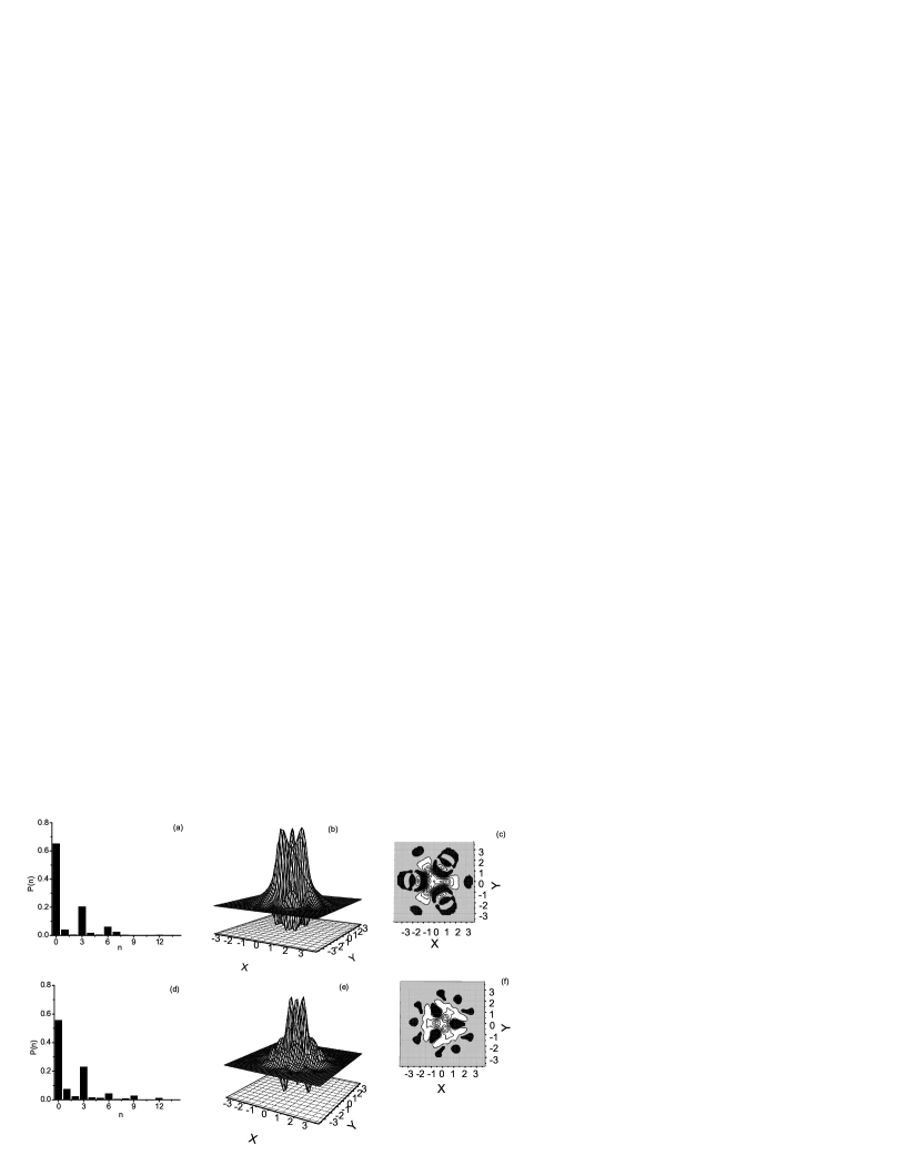
Figure 1: The photon number distributions (a, d), the Wigner functions (b, e) and its contour plots (c, f) for $\omega_{1}$-mode and for different time intervals: $t=t_{0}+6.2*10^{-3}\gamma^{-1}$ (a, b, c); $t=t_{0}+6.2*10^{-2}\gamma^{-1}$ (d, e, f). The other parameters are: $\chi_{1}/\gamma_{1}=200$, $\chi_{2}/\gamma_{1}=100$, $\gamma_{2}=\gamma_{1}=\gamma,T\gamma=1*10^{-3},\tau\gamma=6*10^{-3}$ .

Three-photon structure of the mode is shown on the photon-number distributions in Figs. 1 (a, d). As we see, for short time-intervals, the most probable values of photon numbers are separated by three photons. In Figs.1 (b, e) we present results on the Wigner functions that clearly exhibit phase-space quantum interfringes. These results describe the case of cascaded OPO under two consecutive pulses with the duration $T\gamma=1*10^{-3}$ separated by the time-interval $\tau\gamma=6*10^{-3}$. Fig.1(b) shows the Wigner function evolved for a time interval $t=t_{0}+6.2*10^{-3}\gamma^{-1}$ that corresponds to maximal photon number $n_{max}$ of the first pulse; Fig.1 (e) shows the Wigner function at $t=t_{0}+6.2*10^{-2}\gamma^{-1}$ corresponding to $n_{max}$ of the second pulse. The Wigner function show three phase components with an interference pattern in the regions between them. We show the regions of quantum interference in the contour plots (see, Figs.1 (c, f)) depicting negative regions of the interference terms in black. Note that threefold symmetry of the Wigner function and interference pattern has been demonstrated for the direct three-photon down-conversion in $\chi^{(3)}$ media H6 ; H9 . However, we note that the results presented here for the pulsed cascaded configuration are also different in details from the analogous calculation of the Wigner function for the case of monochromatic pump field Hl7 .

VI Photon-number correlation in the pulsed regime

The experimental verification of time-dependent correlation between photons in triplet has been demonstrated for one-passing configuration of cascaded SPDC Hamel . Considering production of photon triplet in a cavity, it seems that the correlation between photons can be evidently displayed for short interaction time intervals much shorter than the relaxation time. Nevertheless, the three-photon number correlation exceeding the coherent level, (that means the normalized third-order correlation function $g^{(3)}>1$), has been demonstrated for the cascaded OPO driven by monochromatic pumping, in over transient regime for modes generated below the threshold Hl7 . This effect decreases if the system moves to the range of the generation threshold. At the threshold, the typical value for the normalized third-order correlation function for zero delay-time, $g^{(3)}=1.2$ has been obtained.

Note, that effects of two-photon correlations for ordinary OPO and NOPO have been a subject of intense research efforts for last years. These problems have been investigated in details in a linear approximation on quantum fluctuations as well as in the framework of exact quantum theory of intracavity parametric generation with allowance for quantum noise of arbitrary intensity. In this way, the critical behavior of the second-order correlation functions which describe photon correlation effects has been found analytically on the base of the Fokker-Planck equation for the density matrix in the threshold region of generation critic .

In this Secion, we demonstrate the new regimes of strong three-photon correlation for the pulsed cascaded OPO. We concentrate on the numerical simulation of both the mean photon number of subharmonics as well as the third-order correlation function. Let us now discuss photon-number correlation in the time domain, considering output twin light beams from the pulsed cascaded OPO on the base of normalized third-order photon-numbers correlation function $g^{(3)}$ for the mode (1)

$$g^{(3)}(t)=Tr(a_{1}^{+3}a_{1}^{3}\rho_{1}(t))/n^{3}(t).$$ (29)

Here, $n(t)=Tr(a_{1}^{+}a_{1}\rho_{1}(t))$ is the mean photon number. Considering three-photon number correlation for the intensive cavity mode in the presence of dissipation and cavity induced feedback, we control quantum dynamics of dissipative systems by the train of pulses. Here, we use this approach for controlling quantum statistics of mode, particularly for increasing the level of three-photon-number correlation. We analyze the cases in which $T\gamma\leq 1$ and $\tau\gamma\geq 1$, for over transient time-intervals, $t\gg\gamma^{-1}$, considering the operational regimes below-and at the generation threshold. Typical results for the mean photon numbers and the correlation function $g^{(3)}$ for two different parameters of the Gaussian pulses : $T=\gamma^{-1},\tau=10\gamma^{-1}$ and $T=\gamma^{-1},\tau=5\gamma^{-1}$ are presented in Figs. (2) and (4).

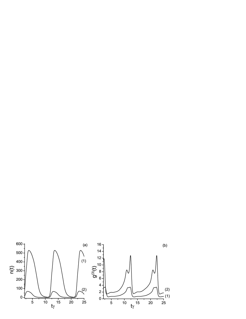
Figure 2: The mean photon number (a) and the third-order correlation function (b) versus $t\gamma$ at the threshold $E_{L}/\overline{E_{th}}=1$, curves (1) and below the threshold $E_{l}/\overline{E_{th}}=0.5$, curves (2). The parameters are: $\chi_{1}/\gamma=0.2$, $\chi_{2}/\gamma=0.1$, $\gamma_{2}=\gamma_{1}=\gamma$, $\tau\gamma=10$, $T\gamma=1$.

Figure 3: Mean photon number (a) and the correlation function (b) for continuously pumped OPO at the threshold $E_{L}/E_{th}=1$. The parameters are: $\chi_{1}/\gamma=0.2$, $\chi_{2}/\gamma=0.1$, $\gamma_{2}=\gamma_{1}=\gamma$.

As we see from these figures, the time-dependence of these quantities repeat the periodicity of the pump laser over transient time intervals. We also conclude that the maxima of the three-photon correlation are realized for the definite time intervals for which the mean photon number of mode (1) is in the ranges between its maxima and minima. As shown our calculations, such strong photon correlations take place in nonstationary regime of cascaded OPO when duration of pulses is close to a characteristic dissipation time. In Figs. (2) we analyze the mean photon number (Fig. 2(a)) and the correlation function (Fig.2(b)) in the operational regimes of OPO below- and at the generation threshold. In the regime below the generation threshold, at $E/\overline{E_{th}}=0.5$ the correlation function display two-peak structure (see, curve (2)). The lower peak corresponds to the time intervals for which the mean photon number is between its minimal and maximal values. More correctly, for the period trains of intervals $t=t_{0}+m11.6\gamma^{-1},(m=1,2,...)$, the mean photon number $n=50$ and the correlation function $g^{(3)}=8.9$. The other peaks correspond to the minimal values of the mean photon number. At the threshold (see, curves (1)) the effect of photon correlation is decreased, although the level of correlation exceeds the coherent level, $g^{(3)}>1$, particularly, we get $g^{(3)}=3.4$ for the mean photon number n=251. Thus, we found a remarkable result that the degree of three-photon number correlation for the pulsed regime of OPO surpass the analogous result for OPO with continuous pumping for the same mean photon numbers. Indeed, this conclusion is illustrated in Figs. (2) and (3), where the comparison of the results on pulsed regime with the calculations based on the Hamiltonian (3) with $f=1$ is done. Note, that the ideal limit of continuous pumping is realized if $T\rightarrow 0,\tau\rightarrow\infty$ for the case of infinity numbers of pulses. We present on the Figs. (3) the results for OPO with continuous pumping at the threshold $E_{L}=E_{th}$, in which the mean photon number $n=52$ in the steady state regime (curve (2), Fig. 2(a)) approximately equals to the maximal value of the photon number in the pulsed regime. However, as we see, the level of the maximal correlation, $g^{(3)}=9$ in this case exceeds the analogous one for the case of continuous pumping, $g^{(3)}=1.2$.

It is natural to explain such improvement of three-photon correlation by control the behavior of a quantum system by an external time-dependent force. The presence of these effects in the cascaded OPO, particularly, can been seen from the noise-correlation functions. Indeed, the equation (10) describes a multiplicative noise-term, where the level of noise is determined by the amplitude of pulsed driving field $E_{L}f(t)$ leading to the control of dissipation. In this spirit, we emphasize that the idea of controlling the dynamics of a quantum system in the presence of dissipation and decoherence by an external periodic driving was exploited by many authors (see, for example, H20 and the references therein). In one of the standard techniques control of the optical quantum system is achieved through the application of suitable tailored, synchronized laser pulses H21 . In this way, it is interesting to analyze the three-photon correlation function in dependence of the time-separation between pulses, i.e. for the other parameters of driving pulses in additional to the parameters considered in Figs. 2. The results are presented in Figs. 4 in the regime below the threshold where strong three-photon correlations are realized. As we see, in this case the correlation function reach to $g^{(3)}=75$ for $n=1.1$ (curves (1)) for time-intervals between pulses, $\tau=10\gamma^{-1}$. Decreasing of the time-separation between pulses leads to decreasing of the correlation function (see, curves (2), where $\tau=5\gamma^{-1}$).

Figure 4: The correlation functions (a) and the mean photon numbers (b) at $E_{L}/\overline{E_{th}}=0.2$ for time-separation between pulses: $\tau\gamma=10$, curves (1) ; $\tau\gamma=5$, curves (2). The parameters are: $\chi_{1}/\gamma=0.2$, $\chi_{2}/\gamma=0.1$, $\gamma_{2}=\gamma_{1}=\gamma$, $T\gamma=1$.

VII Conclusion

In conclusion, we have studied quantum properties of photon triplet cardinally different from those of twin photons. Because photon-triplet originates from a single laser photon, the quantum correlations take place between all three photons allowing the creation of entangled, non-product states. The production of photon-triplets in the presence of stimulation radiative processes, cavity feed-back effects and dissipation have been investigated. We have demonstrated the possibility to create polarization, non-product states of photon-triplet for one-passing, collinear configuration of cascaded parametric spontaneous processes. We have also illustrated three-photon structure of sub-harmonic mode on the base of both the photon-number distribution and the Wigner function. We have demonstrated the operational regimes depending on the durations of pulses and the intervals between them that guarantees strong three-photon-number correlations. This effect of strong correlation takes place for the definite time intervals corresponding to generation of high intensity ”three-photon mode” in over transient regime and for wide ranges of the system parameters. We hope that these results could be of interest in areas of quantum communications and photonic quantum computing.

References

References

- (1) H. H ubel et al 2010 Nature Photonics Lett. 466, 09175.
- (2) D.M. Greenberger, M.A. Horne, and A. Zeilinger, in Bell’s Theorem, Quantum Theory, and Conceptions of the Universe, M. Kafatos, ed. (Kluwer, 1989).
- (3) D. Bouwmeester et al, 1999 Phys. Rev. Lett. 82, 1345; J.-W. Panet al, 2000 Nature (London) 403, 515.
- (4) M. Eibl, N. Kiesel, M. Bourennane, C. Kurtsiefer, and H. Weinfurter, 1998 Phys. Rev. Lett. 92, 077901.
- (5) W.Dr, G. Vidal, and J. I. Cirac, 2000 Phys. Rev. A 62, 062314.
- (6) K.Banaszek and P.Knight, 1997 Phys. Rev. A 55, 2368.
- (7) D.M. Greenberger, M.A. Horne, A. Shimony, and A. Zellinger, 1990 Am. J. Phys. 58, 1131.
- (8) T.E. Keller, M.H. Rubin, Y. Shih, and L.A. Wu, 1998 Phys. Rev. A 57, 2076.
- (9) T. Felbinger, S. Schiller, and J. Mlynek, 1998 Phys. Rev. Lett. 80, 492.
- (10) J. Douady, and B. Boulanger, 2004 Opt. Lett. 29, 2794.
- (11) K. Bencheikh, F. Gravier, J. Douady, J.A. Levenson, and B. Boulanger, 2007 C.R. Phys. 8, 206.
- (12) H.C. Guo, Y.Q. Qin, and S.H. Tang, 2005 Appl. Phys. Lett. 87, 161101.
- (13) J.M. Wen and M. H. Rubin, 2009 Phys. Rev. A 79, 025802.
- (14) J. Wen, E. Oh, and Sh. Du, 2010 J. Opt. Soc. Am. B 27(6), A11.
- (15) G.Yu. Kryuchkyan, N.T. Muradyan, 2001 Phys. Lett. A 286, 113; G.Yu. Kryuchkyan, L.A. Manukyan and N.T. Muradyan, 2001 Opt. Comm. 190, 245.
- (16) J.J. Zondy, A. Tallet, E. Ressayre, and M. LeBerre, 2001 Phys. Rev. A 63, 023814.
- (17) D. A. Antonosyan, T. V. Gevorgyan, and G. Yu. Kryuchkyan, 2011 Phys. Rev. A 83, 043807.
- (18) N. H. Adamyan, H. H. Adamyan, and G. Yu. Kryuchkyan, 2008 Phys. Rev. A 77, 023820.
- (19) N. Gisin and I.C. Percival, 1992 J. Phys. A 25, 5677; I.C. Percival, 2002 Quantum State Diffusion (Cambridge University Press, Cambridge).
- (20) H. H. Adamyan, N. H. Adamyan, N. T. Gevorgyan, T. V. Gevorgyan and G. Yu. Kryuchkyan, 2008 Physics of Particles and Nuclei Letters, 5, 161.
- (21) H. H. Adamyan, S. B. Manvelyan and G. Yu. Kryuchkyan, 2001 Phys. Rev. A 63 022102; S. B. Manvelyan and G. Yu. Kryuchkyan, 2002 Phys. Rev. Lett. 88 094101; T. V. Gevorgyan, A. R. Shahinyan, G. Yu. Kryuchkyan, 2009 Phys. Rev. A 79 094101.
- (22) P. Trojek and H. Weinfurter, Appl. Phys. Lett. 92, 211103 (2008).
- (23) G. Yu. Kryuchkyan, K. V. Kheruntsyan.1996 JEPT 83, 375 ; G. Yu. Kryuchkyan, K. G. Petrossian, K. V. Kheruntsyan. 1996 JEPT Lett 63, 526.
- (24) L. Viola, E. Knill, and S. Lloyd, 1999 Phys. Rev. Lett 82 2414; L. Viola and E. Knill, 2003 Phys.Rev. Lett. 90 037901.
- (25) G.J. Milburn et al 2007 Rev. Mod. Phys. 79, 135.