Towards a cross-correlation approach to strong-field dynamics in Black Hole spacetimes

Abstract

The qualitative and quantitative understanding of near-horizon gravitational dynamics in the strong-field regime represents a challenge both at a fundamental level and in astrophysical applications. Recent advances in numerical relativity and in the geometric characterization of black hole horizons open new conceptual and technical avenues into the problem. We discuss here a research methodology in which spacetime dynamics is probed through the cross-correlation of geometric quantities constructed on the black hole horizon and on null infinity. These two hypersurfaces respond to evolving gravitational fields in the bulk, providing canonical ”test screens” in a ”scattering”-like perspective onto spacetime dynamics. More specifically, we adopt a 3+1 Initial Value Problem approach to the construction of generic spacetimes and discuss the role and properties of dynamical trapping horizons as canonical inner ”screens” in this context. We apply these ideas and techniques to the study of the recoil dynamics in post-merger binary black holes, an important issue in supermassive galactic black hole mergers.

1 A cross-correlation approach: Motivations and Objective

The general problem here discussed is the qualitative and quantitative understanding of near-horizon gravitational dynamics in the strong-field regime of black hole (BH) spacetimes. This represents a challenge both at a fundamental level and in astrophysical applications. The setting of our discussion is that of classical spacetimes in General Relativity (GR), with a focus on astrophysically motivated problems in which we adopt a numerical relativity methodology.

A natural strategy to the study of spacetime dynamics consists in extending to the general relativistic setting the Newtonian description of the dynamics of gravitationally interacting bodies, namely celestial mechanics. This has proved extremely successful in unveiling the physics of compact objects. However, such an approach also meets fundamental obstacles in the general dynamical regime of a gravitational theory in which i) a priori rigid structures providing canonical references (such as symmetries or preferred backgrounds) are generically absent, and ii) where global aspects play a crucial role. Here we rather adopt a complementary approach in the spirit of a coarse-grained description of the dynamics in which we renounce to the detailed tracking of the geometry (trajectories) of given compact regions (objects), and rather emphasize the global/quasi-local properties of the relevant dynamical fields. In particular, we aim at capturing the functional structure of the latter through appropriate correlation functions.

From a physical perspective, we focus on what is sometimes called the “establishment’s picture of gravitational collapse” Penrose (1973). Our current understanding of this problem can be summarized in the following chain of theorems and conjectures:

• Singularity theorems Penrose (1965); Hawking (1967); Hawking and Penrose (1970); Hawking and Ellis (1973): if sufficient energy is placed in a sufficiently compact spacetime region, light locally converges in any emitted direction, trapped surfaces form and a spacetime singularity develops in their causal future.

• Weak cosmic censorship conjecture Penrose (1969): to preserve predictability, the singularity is hidden from a distant observer behind an event horizon giving rise to a BH region.

• BH spacetime stability (conjecture): GR dynamics drive the system to stationarity.

• BH uniqueness (theorem) Heusler (1998): the final state is a subextremal Kerr BH spacetime.

The establishment’s picture of gravitational collapse is an intrinsically dynamical picture. Accordingly, we adopt a methodology able to cope with the construction and analysis of generic spacetimes, namely in an Initial Value Problem approach. This provides a systematic avenue to the study of the qualitative and quantitative aspects of generic dynamical spacetimes, respectively addressed through the use of tools in Partial Differential Equation theory and by the numerical construction of spacetimes.

Our focus is on the point iii) above, in an attempt to gain insight into the specific manner in which GR drives the system eventually to stationarity. Remarkably, tools devised in the study of i) and ii) (namely, the characterizations of BH horizons) prove to be very useful to reach this goal. In this sense, a crucial outcome of the systematic numerical exploration of fully dynamical vacuum spacetimes in recent years is that the a posteriori description of gravitational dynamics is rather simple. This specific observation is the main point supporting the applicability of a coarse-grained approach to the analysis of generic spacetime dynamics.

1.1 A cross-correlation approach to BH spacetime dynamics

In order to make concrete the previous considerations, we formulate the following cross-correlation methodology Jaramillo et al. (2011a, b); Jaramillo (2011), whose specific goal is the development of qualitative insights into spacetime dynamics in the strong-field regime, identifying the key elements leading ultimately to appropriate quantitative effective descriptions:

• Spacetime dynamics is probed through the cross-correlation of geometric quantities $h_{\mathrm{inn}}$ an $h_{\mathrm{out}}$ defined at inner and outer hypersurfaces, respectively, ${\cal H}_{\mathrm{inn}}$ and ${\cal H}_{\mathrm{out}}$.

• Hypersurfaces ${\cal H}_{\mathrm{inn}}$ and ${\cal H}_{\mathrm{out}}$ are taken as test screens responding to bulk dynamics. Spacetime is then explored in the spirit of an ”inverse scattering approach”.

In our near-horizon and asymptotically flat context, the BH event horizon ${\cal E}$ and future null infinity ${I}^{+}$ provide natural choices, respectively, for ${\cal H}_{\mathrm{inn}}$ and ${\cal H}_{\mathrm{out}}$ (cf. Fig. 1). Quantities $h_{\mathrm{inn}}(v)$ and $h_{\mathrm{out}}(u)$ are then constructed on ${\cal E}$ and ${I}^{+}$ as functions, respectively, of appropriate advanced and retarded times. We note that the cross-correlations (as time-series) between $h_{\mathrm{inn}}(v)$ and $h_{\mathrm{out}}(u)$ require a gauge mapping between $v$ and $u$.

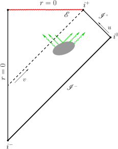
Figure 1: Sketch of the conformal diagram for a spherically symmetric gravitational collapse, illustrating the scenario for the cross-correlation approach to the analysis of bulk spacetime dynamics.

2 BH horizons: Global vs. Quasi-local approaches

BH horizons play a crucial role in our discussion, offering in particular a model for the inner hypersurface ${\cal H}_{\mathrm{inn}}$ in the cross-correlation scheme. Two approaches to the BH notion can be considered, both contained in the the standard picture of gravitational collapse. The first one is guaranteed by weak cosmic censorship: the black hole region $\mathcal{B}$ is a region of no-escape not extending up to infinity. In a strongly asymptotically predictable spacetime ${\cal M}$, with $J^{-}({I}^{+})$ denoting the causal past of ${I}^{+}$, we have $\mathcal{B}={\cal M}-J^{-}({I}^{+})$. The boundary of the black region is given by the event horizon $\mathcal{E}={\partial{J}}^{-}({I}^{+})\cap{\cal M}$. This traditional characterization of BHs for asymptotically flat spacetimes involves global spacetime concepts. In particular, event horizons $\mathcal{E}$ are teleological objects whose location requires the full knowledge of the spacetime in the future and that can develop in flat regions. Event horizons are therefore not adapted for probing the BH spacetime during its construction in an Initial Value Problem approach.

Alternatively, instead of characterizing the BH as the region that cannot send signals to distant observers, we can approach it as the region where all emitted light rays “locally converge”. This is made precise by the notion of trapped surface, crucial in the singularity theorems appearing in the standard gravitational collapse picture. Given a closed surface ${\cal S}\subset{\cal M}$ with area element $dA=\sqrt{q}\;d^{2}x$, its normal plane can be spanned in terms of an outgoing null vector $\ell^{a}$ and an ingoing null vector $k^{a}$. The outgoing expansion $\theta^{(\ell)}$ measures the rate of change of $dA$ in the lightfronts emitted from ${\cal S}$ along the outgoing null direction $\ell^{a}$. The ingoing expansion $\theta^{(k)}$ is defined analogously

$$\theta^{(\ell)}\equiv\frac{1}{\sqrt{q}}{\cal L}_{\ell}\sqrt{q}\ \ \ ,\ \ \ \theta^{(k)}\equiv\frac{1}{\sqrt{q}}{\cal L}_{k}\sqrt{q}\ \ .$$ (1)

Then ${\cal S}$ is a (future) trapped surface Penrose (1965) if $\theta^{(\ell)}<0$ and $\theta^{(k)}<0$. The limiting case in which one of the expansion vanishes defines a marginally trapped surface: $\theta^{(\ell)}=0$, $\theta^{(k)}<0$. If there exists a notion of outer region, e.g. associated with an asymptotically flat region, then (future) outer trapped surfaces Hawking and Ellis (1973) can be introduced as $\theta^{(\ell)}<0$, without any requirement on $\theta^{(k)}$. A marginally outer trapped surface satisfies then $\theta^{(\ell)}=0$. In this context the BH can be characterized in terms of the trapped region ${\cal T}$, namely the set of points in spacetime belonging to some trapped surface. In the present context of a cross-correlation analysis, rather than in the BH or trapped region themselves we are primarily interested in its boundary. The latter provides a hypersurface to be employed as an inner screen ${\cal H}_{\mathrm{inn}}$. In this sense, the so-called trapping boundary Hayward (1994), namely the boundary of the trapped region ${\cal T}$, would be a good candidate for ${\cal H}_{\mathrm{inn}}$. Unfortunately, we lack an operational characterization of such trapping boundary. This is in contrast with the notion of apparent horizon, namely the boundary of the trapped region contained in a given 3-slice $\Sigma$, characterized as a marginally outer trapped surface $\theta^{(\ell)}=0$. Motivated by these difficulties, trapping horizons (namely worldtubes of marginally outer trapped surfaces) were introduced Hayward (1994) as quasi-local models for the BH horizon, in particular in an attempt to gain insight about the trapping boundary.

3 Quasi-local horizons as inner test screens

We review the properties of dynamical trapping horizons, stressing those aspects of special relevance in our discussion. Let us consider a closed orientable 2-surface ${\cal S}$ embedded in a 4-dimensional spacetime $({\cal M},g_{ab})$, with Levi-Civita connection $\nabla_{a}$. Regarding its intrinsic geometry, we denote the induced metric as $q_{ab}$, with Levi-Civita connection $D_{a}$, Ricci scalar ${}^{2}\!R$ and area form $\epsilon_{ab}$ (area measure $dA$). Again, normal outgoing and ingoing null normals are denoted as $\ell^{a}$ and $k^{a}$, normalized as $\ell^{a}k_{a}=-1$. This leaves a (boost) rescaling freedom $\ell^{\prime a}=f\ell^{a}$, $k^{\prime a}=f^{-1}k^{a}$, with $f$ a function on ${\cal S}$.

We need the following elements of the extrinsic geometry. The outgoing expansion $\theta^{(\ell)}$, given in Eq. (1), and the outgoing shear $\sigma^{(\ell)}_{ab}$ are expressed as

$$\theta^{(\ell)}=q^{ab}\nabla_{a}\ell_{b}\ \ \ \ ,\ \ \ \ \sigma^{(\ell)}_{ab}={q^{c}}_{a}{q^{d}}_{b}\nabla_{c}\ell_{d}-\frac{1}{2}\theta^{(\ell)}q_{ab}\ ,$$ (2)

whereas a normal fundamental 1-form $\Omega^{(\ell)}_{a}$ associated with $\ell^{a}$ is given by

$$\Omega^{(\ell)}_{a}=-k^{c}{q^{d}}_{a}\nabla_{d}\ell_{c}\ ,$$ (3)

provides a connection on $T^{\perp}{\cal S}$. The transformation of these quantities under a null rescaling are: $\theta^{(\ell^{\prime})}=f\theta^{(\ell)}$, $\sigma^{(\ell^{\prime})}_{ab}=f\sigma^{(\ell)}_{ab}$ and $\Omega^{(\ell^{\prime})}_{a}=\Omega^{(\ell)}_{a}+D_{a}(\mathrm{ln}f)$. Finally, we need to control the variations of the outgoing expansion $\theta^{(\ell)}$ along normal vectors $v^{a}\in T^{\perp}{\cal S}$

$$\delta_{\alpha\ell}\theta^{(\ell)} = \kappa^{(\alpha\ell)}\theta^{(\ell)}-\alpha\left[\sigma^{(\ell)}_{ab}{\sigma^{(\ell)}}^{ab}+G_{ab}\ell^{a}k^{b}+\frac{1}{2}\left(\theta^{(\ell)}\right)^{2}\right]$$

$$\delta_{\beta k}\theta^{(\ell)} = \kappa^{(\beta k)}\theta^{(\ell)}+{}^{2}\!\Delta\beta-2\Omega^{(\ell)}_{a}D^{a}\beta$$ (4)

$$+\beta\left[\Omega^{(\ell)}_{a}{\Omega^{(\ell)}}^{a}-D^{a}\Omega^{(\ell)}_{a}-\frac{1}{2}{}^{2}\!R+G_{ab}k^{a}\ell^{b}-\theta^{(\ell)}\theta^{(k)}\right]\ ,$$

where $\kappa^{(v)}=-v^{a}k^{b}\nabla_{a}\ell_{b}$, $\alpha$ and $\beta$ are functions on ${\cal S}$ and $\delta_{v}$ is the variation operator associated with a change in the underlying surface ${\cal S}$ (cf. Andersson et al. (2005, 2008); Booth and Fairhurst (2007)).

A trapping horizon Hayward (1994) is (the closure of) a hypersurface ${\cal H}$ foliated by closed marginally outer trapped surfaces: ${\cal H}=\bigcup_{t\in\mathbb{R}}{\cal S}_{t}$, with $\theta^{(\ell)}=0$. The properties of ${\cal H}$ as a horizon are characterized by the signs of $\theta^{(k)}$ and $\delta_{k}\theta^{(\ell)}$: i) the sign of $\theta^{(k)}$ controls if the singularity occurs in the future ($\theta^{(k)}<0)$ or in the past ($\theta^{(k)}>0)$, and ii) the sign of $\delta_{k}\theta^{(\ell)}$ controls the (local) outer ($\delta_{k}\theta^{(\ell)}<0$) or inner ($\delta_{k}\theta^{(\ell)}>0$) character of ${\cal H}$ with respect to the trapped region. For BHs the singularity occurs in the future and the horizon is an outer boundary. Therefore quasi-local BH horizons are modeled by future outer trapping horizons (FOTH): $\theta^{(\ell)}=0$, $\theta^{(k)}<0$ and $\delta_{k}\theta^{(\ell)}<0$.

We can define an evolution vector $h^{a}$ on ${\cal H}$ characterized by: i) $h^{a}$ is tangent to ${\cal H}$ and orthogonal to ${\cal S}_{t}$, ii) $h^{a}$ transports ${\cal S}_{t}$ to ${\cal S}_{t+\delta t}$: ${\cal L}_{h}t=1$, and iii) $h^{a}$ is written as $h^{a}=\ell^{a}-Ck^{a}$. We also define a dual vector $\tau^{a}=\ell^{a}+Ck^{a}$ orthogonal to ${\cal H}$. The sign of $C$ fixes the point-like metric type of ${\cal H}$: $C>0$ spacelike, $C=0$ null, $C<0$ timelike. Considering first the spherically symmetric case ($C$ constant on ${\cal S}_{t}$), the trapping horizon conditions $\theta^{(\ell)}=0$, $\delta_{h}\theta^{(\ell)}=0$ imply, using Eq. (3) and Einstein equations

$$C=-\frac{\sigma_{ab}^{(\ell)}{\sigma^{(\ell)}}^{ab}+T_{ab}\ell^{a}\ell^{b}}{\delta_{k}\theta^{(\ell)}}\geq 0\ ,$$ (5)

for an outer ${\cal H}$ (i.e. $\delta_{k}\theta^{(\ell)}<0$) under the null energy condition. Therefore FOTHs ${\cal H}$ can be either null or spacelike hypersurfaces. The first case corresponds to the stationary regime (with its the isolated horizon hierarchy Ashtekar and Krishnan (2004); Gourgoulhon and Jaramillo (2006a)), whereas the second case leads to dynamical horizons (DHs) Ashtekar and Krishnan (2002, 2003). Beyond spherical symmetry, one can pose the question if a MOTS section ${\cal S}_{t}$ of a FOTH can be partially spacelike and partially null, i.e. if it can happen $C>0$ in a part of ${\cal S}_{t}$ and $C=0$ in another part. The answer is in the negative: transitions from stationarity to the dynamical regime happens “all at once” in sections ${\cal S}_{t}$ of ${\cal H}$. This follows from the trapping horizon condition written as [use (3)]

$$\delta_{h}\theta^{(\ell)}=-{}^{2}\!D_{c}{}^{2}\!D^{c}C+2{\Omega^{(\ell)}}^{c}{}^{2}\!D_{c}C-C\delta_{k}\theta^{(\ell)}+\delta_{\ell}\theta^{(\ell)}=0\ .$$ (6)

Under an outer condition $\delta_{k}\theta^{(\ell)}<0$, a maximum principle can be applied to this elliptic equation to conclude that either $C>0$ (if $\delta_{\ell}\theta^{(\ell)}=\sigma_{ab}^{(\ell)}{\sigma^{(\ell)}}^{ab}+T_{ab}\ell^{a}\ell^{b}\neq 0$ at some point of ${\cal S}_{t}$), or $C=0$ if and only if $\delta_{\ell}\theta^{(\ell)}=0$ everywhere on ${\cal S}_{t}$. In other words, it suffices that some energy crosses the horizon at a single point, for making the whole horizon grow globally. This non-local behaviour is encoded in the elliptic nature of Eq. (6), providing an example of the non-local behaviour of these dynamical trapping horizons. This is possibly disturbing, if considering ${\cal H}$ as the boundary of a physical object. An even more curious behaviour of ${\cal H}$ follows from the two following results:

• Foliation uniqueness Ashtekar and Galloway (2005): the foliation by MOTSs of a dynamical FOTH is unique.

• Existence of DHs Andersson et al. (2005, 2008): Given a (stable) marginally outer trapped surface ${\cal S}_{0}$ in a Cauchy hypersurface $\Sigma_{0}$, to each 3+1 spacetime foliation $(\Sigma_{t})_{t\in\mathbb{R}}$ containing $\Sigma_{0}$ it corresponds a unique adapted dynamical FOTHs ${\cal H}$ that contains ${\cal S}_{0}$ and is sliced by marginally outer trapped surfaces $\{{\cal S}_{t}\}$ such that ${\cal S}_{t}\subset\Sigma_{t}$.

The first result provides a sort of rigidity for DHs, very useful in our context since it determines the evolution vector $h^{a}$ uniquely up to a time reparametrization. Regarding the second result, this is a crucial benchmark in the treatment of quasi-local horizons in an Initial Value Problem approach. The main point we want to underline here is that the combination of results i) and ii) above leads to the non-uniqueness of DHs: the combination of results on evolution existence and foliation uniqueness for DHs implies the generic non-uniqueness in the evolution of a FOTH from an initial MOTS. To see this it suffices to consider the evolution of an initial ${\cal S}_{0}\in\Sigma_{0}$ into DHs ${\cal H}_{1}$ and ${\cal H}_{2}$ compatible with (generic) 3+1 foliations $\{\Sigma_{t_{1}}\}$ and $\{\Sigma_{t_{2}}\}$, assume ${\cal H}_{1}={\cal H}_{2}$ and then reason by contradiction with the result on the uniqueness of the foliation (see e.g. Jaramillo et al. (2011b)). Such non-uniqueness in the evolution is a surprising behaviour if we consider ${\cal H}$ as the boundary of a physical object. Actually such behaviour is a characteristic signature of gauge dynamics. At this point it is worth to remark that the amount of gauge freedom in the stationary and the dynamical cases remains the same: whereas i) in equilibrium the geometric hyperfurface ${\cal H}$ is unique, but its foliation by MOTS is not unique and can be parametrized by a free function $f$ on ${\cal S}$ rescaling the null normal ($\ell^{a}\rightarrow f\ell^{a}$), ii) in the dynamical case the geometric hypersurface is non-unique but the foliation by MOTS is rigid. In this latter case, the gauge freedom is given by the choice 3+1 foliation, i.e. by the lapse function $N$ evaluated on ${\cal S}$. Therefore, both equilibrium and dynamical cases present the gauge freedom (the choice of a function on ${\cal S}$), but dressed differently.

3.1 A pragmatical view on FOTHs

From the discussion above we must retain: i) FOTHs are hypersurfaces tracking the BH region, ii) they are well-adapted to the 3+1 Initial Value Problem approach, and iii) DHs incorporate a sort of rigidity fixing the evolution vector up to time reparametrization. These are remarkable geometric properties. If considered as physical surfaces, FOTHs present curious properties: i) non-uniqueness, ii) superluminal behaviour (when dynamical) and iii) global behaviour. The last point has been addressed in detail in Ref. Bengtsson and Senovilla (2011), where clairvoyance properties of trapped surfaces are discussed, in particular their capacity to enter into flat regions, one of the reasons to abandon event horizons.

Although dynamical trapping horizons have proved very useful to gain crucial insight into physical aspects such as BH thermodynamics in dynamical contexts Ashtekar and Krishnan (2004); Hayward (1994), for the reasons discussed above we adopt here a perspective underlining the role of FOTHs as purely geometric probes to be employed the analysis of dynamical spacetimes. When considering an inner test screen ${\cal H}_{\mathrm{inn}}$ in the context of the cross-correlation approach, we look for a hypersurface that: i) should be a footprint of the BH presence, in particular providing a probe into their spacetime geometry, ii) should be suitable for the Initial Value Problem approach, providing in this setting a preferred geometrically defined structure with some sort of rigidity, and iii) should intrinsically incorporate an evolution concept, tracking the evolution of the BH properties. In this context, we adopt a pragmatical approach on DHs, as hypersurfaces of remarkable geometric properties in BH spacetimes, providing preferred geometric probes into the BH spacetime geometry.

3.2 Initial Value Problem and cross-correlation approaches

The adoption of an Initial Value Problem approach to the construction of the spacetime has an impact on the cross-correlation scheme sketched above. On the one hand, as already discussed, the event horizon ${E}$ is not available during the evolution. In addition, in a Cauchy evolution of an asymptotically flat spacetime one does not constructs null infinity ${I}^{+}$, but rather the slices $\Sigma_{t}$ reach spatial infinity $i^{0}$ (as an alternative, one could solve a hyperboloidal Initial Boundary Value Problem, rather than a Cauchy one, to construct ${I}^{+}$). On the other hand, advanced and retarded times $u$ and $v$ are not natural, and one rather employ a 3+1 time function $t$ associated with the slicing $\{\Sigma_{t}\}$.

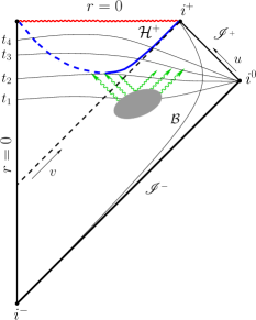
Figure 2: Illustration of the use of the Initial Value Problem approach in the cross-correlation scheme. A DH is used as inner screen ${\cal H}_{\mathrm{inn}}$, whereas the large spheres world-tube ${\cal B}$ (or ${I}^{+}$) is used for ${\cal H}_{\mathrm{out}}$.

Therefore, in our 3+1 treatment of the cross-correlation methodology we shall employ (cf. Fig. 2): i) dynamical trapping horizons as canonical inner screens associated with the 3+1 slicing with lapse function $N$, ii) a timelike worldtube ${\cal B}$ at large distances as outer screen (or ${I}^{+}$ in a hyperboloidal slicing), and iii) a 3+1 spacetime slicing time function $t$ that automatically implements a (gauge) mapping between $u$ and $v$.

In the context of the cross-correlation of quantities $h_{\mathrm{inn}}(t)$ and $h_{\mathrm{out}}(t)$ as time series, we note that generically the 3+1 slices $\Sigma_{t}$ intersect multiply the dynamical trapping horizon (cf. Fig. 2). This is the underlying reason for the jumps occurring in the evolution of apparent horizons, generic in 3+1 BH evolutions. From the 3+1 perspective both an external ${\cal H}_{\mathrm{ext}}$ and an internal ${\cal H}_{\mathrm{int}}$ apparent horizon are present. In numerical simulations it is standard to neglect the internal horizon as irrelevant. The splitting of the single spacetime hypersurface ${\cal H}$ in two parts, ${\cal H}={\cal H}_{\mathrm{int}}\cup{\cal H}_{\mathrm{ext}}$ is an artifact of the 3+1 description and simply reflects that the coordinate $t$ is not a good label for ${\cal H}$. If we are interested in cross-correlations only after the moment $t_{c}$ of first appearance of the apparent horizon, then using the external part ${\cal H}_{\mathrm{ext}}$ is enough. But if integrating fluxes in time is relevant in our problem, then the internal ${\cal H}_{\mathrm{int}}$ must be kept into the picture in order to account for the whole history of the flow into the BH singularity (cf. Fig. 3).

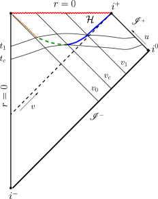
Figure 3: Internal and external apparent horizons in a 3+1 BH evolution. After the moment $t_{c}$ of first appearance, slices $\Sigma_{t}$ intersect multiply the DH ${\cal H}$, splitting it into ${\cal H}_{\mathrm{ext}}$ and ${\cal H}_{\mathrm{int}}$ (dashed line) parts.

4 Application to Black Hole recoil dynamics

We apply now the previous ideas to the study of the recoil dynamics of the BH resulting from the asymmetric merger of two BHs. In an asymmetric binary merger the emission of linear momentum through gravitational waves is not isotropic, so that the final remnant must recoil in order to preserve the total linear momentum. This is astrophysically relevant in the context of the merger of supermassive BHs in galaxy encounters.

We aim at gaining insight into the dynamics controlling the recoil (kick) velocity $v_{\mathrm{k}}$ and, in particular, into the systematics of a late-time deceleration referred to as the anti-kick in the literature. On the one hand, the very presence of such final deceleration is a direct consequence of the fact that the kick velocity is obtained upon integration of a decaying oscillating quantity, namely the flux of linear Bondi momentum at null infinity: there is no reason to expect that the maximum and the asymptotic value of the time integral of a decaying oscillating signal coincide Sperhake et al. (2011). The relevance of this problem lays, rather than on the presence itself of the anti-kick, on the capability to estimate a priori its magnitude from an understanding of the underlying dynamics. In particular, a relative large antikick reduces the resulting kick velocity, whereas large final recoil velocities are associated with small relative antikicks. In this context, the magnitude of the antikick is controlled by the ratio between the oscillation timescale, $T$, and the decaying timescale, $\tau$, leading to the crucial notion of slowness parameter Price et al. (2011)

$$P=\frac{T}{\tau}\ \ ,$$ (7)

so that for $P\ll 1$ the rapid oscillations in the signal induce cancellations in the time integral and lead to large antikicks, whereas for $P\approx 1$ the antikick is small.

Understanding the involved oscillating and decaying dynamics is therefore crucial in this problem. Ref. Rezzolla et al. (2010) paved the way to get insight into the responsible gravitational dynamics, in terms of the analysis of the evolution (dissipation) of the quasi-local horizon geometry. The cross-correlation scheme Jaramillo et al. (2011a, b); Jaramillo (2011) permits to develop a more systematic analysis along those lines. Before proceeding further, and since it will be relevant later, we note that quasi-local BH horizon tools have already been applied to this problem. In particular, Ref. Krishnan et al. (2007) proposes an expression for the BH linear momentum

$$P[\xi]=\frac{1}{8\pi}\int_{{\cal S}_{t}}\left(K_{ab}-K\gamma_{ab}\right)\xi^{a}s^{b}\;dA\ ,$$ (8)

by applying the ADM prescription at spatial infinity $i^{0}$ to the apparent horizon.

4.1 Cross-correlations in BH recoil dynamics

In the application of the cross-correlation approach to BH recoil dynamics, we take as quantity $h_{\mathrm{out}}$ the flux of Bondi linear momentum at ${I}^{+}$ (actually at the approximation given by large spheres worldtube ${\cal B}$) along a spatial direction $\xi^{a}$. That is

$$\frac{dP^{\mathrm{B}}[\xi]}{dt}(t)=\lim\limits_{r\to\infty}\frac{r^{2}}{16\pi}\oint_{{\cal S}_{t,r}}(\xi^{i}s_{i})\left|{\cal N}(t)\right|^{2}d\Omega\ \ \ \ ,\ \ \ \ {\cal N}(t)=\int_{-\infty}^{t}\Psi_{4}(t^{\prime})dt^{\prime}\ ,$$ (9)

where ${\cal N}(t)$ is the so-called news function. At the inner DH screen ${\cal H}$, we lack a geometric analogue to $dP^{\mathrm{B}}[\xi]/dt$, in particular no news function formalism is available. However, Eq. (9) suggests a natural heuristic candidate $\tilde{K}[\xi]$ for the quantity $h_{\mathrm{inn}}$

$$\tilde{K}[\xi](t)\equiv-\frac{1}{16\pi}\oint_{{\cal S}_{t}}(\xi^{i}s_{i})\left|\tilde{\cal N}_{\Psi}^{(\ell)}(t)\right|^{2}dA\ \ \ \ ,\ \ \ \ \tilde{\cal N}_{\Psi}(t)\equiv\int_{t_{0}}^{v}\Psi^{N}_{0}(t^{\prime})dt^{\prime}\ ,$$ (10)

where the Weyl scalar $\Psi^{N}_{0}$ plays the analogous role at ${\cal H}_{\mathrm{inn}}$ that $\Psi_{4}$ plays at ${\cal H}_{\mathrm{out}}$ (the superindex $N$ refers to a choice of null tetrad adapted to the 3+1 foliation with lapse function $N$ Jaramillo et al. (2011b)). However, the function $\tilde{\cal N}_{\Psi}(t)$ does not satisfy a key requirement on the news function, namely its characterization purely in terms of the geometry of a section ${\cal S}_{t}$ of the horizon. In other words, the flux defined by the square of the news must be an instantaneous quantity defined by quantities crossing the horizon at a given time. This issue can be addressed by correcting the integrand in $\tilde{\cal N}_{\Psi}(t)$ with terms completing $\Psi_{0}(t^{\prime})$ to a total time derivative. From the tidal equation for the evolution of the shear $\sigma^{(h)}_{ab}$ along ${\cal H}$, with leading order given by $\Psi^{N}_{0}$, we propose the more geometric quantity

$$\frac{dP^{{}^{({\cal H})}}[\xi]}{dt}(t)=-\frac{1}{16\pi}\oint_{{\cal S}_{t}}(\xi^{i}s_{i})\left({\cal N}^{{}^{({\cal H})}}_{ab}{\cal N}^{{}^{({\cal H})}ab}\right)dA\,,\qquad{\cal N}^{{}^{({\cal H})}}_{ab}\equiv-\frac{1}{\sqrt{2}}\sigma^{(h)}_{ab}\ \ .$$ (11)

The notation $dP^{{}^{({\cal H})}}[\xi]/dt$ is meant to underline that this quantity is well defined at ${\cal S}_{t}$, without implying the existence of a well-defined conserved quantity $P^{{}^{({\cal H})}}$.

The idea now would be to cross-correlate quantities $(dP^{{}^{({\cal H})}}[\xi]/dt)(t)$ at ${\cal H}$ and $(dP^{\mathrm{B}}[\xi]/dt)(t)$ at ${I}^{+}$. This requires however the determination of the evolution vector $h^{a}$, which involves the resolution at each time step of the elliptic Eq. (6) for $C$. Although no conceptual issues are involved in this, we adopt in a first stage a technically simpler strategy where for $h_{\mathrm{inn}}$, rather than $dP^{{}^{({\cal H})}}[\xi]/dt$, we use an effective curvature vector constructed in terms of the intrinsic geometry of ${\cal S}_{t}$. In order to justify this, we write

$$\delta_{h}{}^{2}\!R=-\theta^{(h)}\,{}^{2}\!R+2\;{}^{2}\!D^{a}{}^{2}\!D^{b}\sigma^{(h)}_{ab}-{}^{2}\!\Delta\theta^{(h)}\ ,$$ (12)

for the evolution of the Ricci scalar ${}^{2}\!R$ of the induced metric $q_{ab}$ on ${\cal S}_{t}$. To fully control its evolution, we need to track the evolution of $q_{ab}$, $\theta^{(\ell)}$ and $\sigma^{(h)}_{ab}$. In order to get insight into the involved quantities, we make explicit the system for a null horizon (the actual spacelike case has the same structure, but involving corrections on the function $C$). Then

$$\delta_{\ell}{}^{2}\!R = -\theta^{(\ell)}\,{}^{2}\!R+2\;{}^{2}\!D^{a}{}^{2}\!D^{b}\sigma^{(\ell)}_{ab}-{}^{2}\!\Delta\theta^{(\ell)}$$

$$\delta_{\ell}q_{ab} = 2\sigma^{(\ell)}_{ab}+\theta^{(\ell)}q_{ab}$$

$$\delta_{\ell}\theta^{(\ell)} = -\frac{1}{2}(\theta^{(\ell)})^{2}-\sigma^{(\ell)}_{ab}{\sigma^{(\ell)}}^{ab}-8\pi T_{ab}\ell^{a}\ell^{b}$$ (13)

$$\delta_{\ell}\sigma^{(\ell)}_{ab} = \sigma^{(\ell)}_{cd}{\sigma^{(\ell)}}^{cd}q_{ab}-{q^{c}}_{a}{q^{d}}_{b}C_{lcfd}\ell^{l}\ell^{f}\ \ ,$$

where ${C^{a}}_{bcd}$ denotes the Weyl tensor. Once initial data are given, the whole system is driven by the external forces given by ${q^{c}}_{a}{q^{d}}_{b}C_{lcfd}\ell^{l}\ell^{f}$ and $T_{ab}\ell^{a}\ell^{b}$. Focusing here on the vacuum case (see Jaramillo et al. (2011b) for a more general discussion) we note that ${q^{c}}_{a}{q^{d}}_{b}C_{lcfd}\ell^{l}\ell^{f}=\Psi_{0}\overline{m}_{a}\overline{m}_{b}+\overline{\Psi}_{0}m_{a}m_{b}$, where $m^{a}$ is a complex null vector tangent to ${\cal S}_{t}$. On the one hand, the evolution of the whole system (4.1) is determined by the $\Psi_{0}$ at the horizon, which justifies the understanding of ${\cal N}^{{}^{({\cal H})}}_{ab}$ in Eq. (11) as a kind of news-like function. On the other hand, we note that the evolution of ${}^{2}\!R$ is completely driven by the rest of the system, without backreacting on it. This last point is crucial, since the evolution of ${}^{2}\!R$ then captures in an effective way and in a single function the evolution of the whole system, in particular the evolution of the shear (but also other degrees of freedom if matter is present). This leads to the introduction of the effective curvature vector Jaramillo et al. (2011a)

$$\tilde{K}^{\mathrm{eff}}[\xi](t)\equiv-\frac{1}{16\pi}\oint_{{\cal S}_{t}}(\xi^{i}s_{i})|\tilde{\cal N}(t)|^{2}dA\ \ \ \ ,\ \ \ \ \tilde{\cal N}(t)\equiv\int_{t_{c}}^{t}{}^{2}\!R(t^{\prime})dt^{\prime}+\tilde{\cal N}^{t_{c}}\ \ ,$$ (14)

as an effective estimator of the evolution of the horizon geometry (here $\tilde{\cal N}^{t_{c}}$ is an initial value function; see Jaramillo et al. (2011a) for details on its fixing). In a first stage of our quantitative analysis, we use $\tilde{K}^{\mathrm{eff}}[\xi]$ as the quantity $h_{\mathrm{inn}}$ to be cross-correlated with $dP^{\mathrm{B}}[\xi]/dt$.

In order to test these tools, we have considered the head-on collision of non-spinning black holes with mass ratio $q=1/2$ and have constructed numerically the associated dynamical spacetime (cf. details in Jaramillo et al. (2011a)). We extract the timeseries corresponding to $\tilde{K}^{\mathrm{eff}}[\xi](t)$, once the common apparent horizon has formed and $(dP^{\mathrm{B}}[\xi]/dt)(t)$ at (an approximation to) null infinity during the whole evolution. From a qualitative perspective, both timeseries show a good agreement, from the moment of first appearance of the common apparent horizon. The qualitative agreement is preserved in time (see Fig. 4).

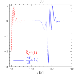
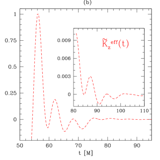
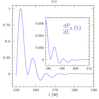
Figure 4: Effective curvature $\tilde{K}^{\mathrm{eff}}_{z}(t)$ at the horizon from the moment of formation of a common horizon (red dashed curve) and flux of Bondi linear momentum $(dP^{\mathrm{B}}[\xi]/dt)(t)$ evaluated at an approximation of ${I}^{+}$ (blue dotted solid curves, before and after the appearance of a common horizon, respectively). Panel (a) shows the good qualitative agreement between both quantities after the merger. Panels b) and (c) compare the same quantities for latter times, showing the persistance in time of the good agreement.

For a quantitative comparison we use the cross-correlation of $h_{1}(t)$ and $h_{2}(t)$

$$\mathrm{Corr}(h_{1},h_{2};\tau) = \int_{-\infty}^{\infty}h_{1}(t+\tau)h_{2}(t)dt\ \ ,$$ (15)

which encodes a quantitative comparison between the two timeseries as a function of the time-shift $\tau$ (lag) between them. In particular, the matching between the two signals can be expressed in terms of the number

$${\cal M}(h_{1},h_{2})=\max\limits_{\tau}\left(\frac{\mathrm{Corr}(h_{1},h_{2})(\tau)}{\left[\mathrm{Corr}(h_{1},h_{1})(0)\cdot\mathrm{Corr}(h_{2},h_{2})(0)\right]^{\frac{1}{2}}}\right)\ \ .$$ (16)

This number is confined between $0$ and $1$ (with $1$ indicating perfect correlation, and $0$ no correlation at all) and provides the maximum matching between the timeseries. The calculation of the correlations in our scheme requires a careful treatment of what can be referred to as a time stretch issue, in order to deal with the freedom in the choice of spacetime foliation that determines the gauge mapping between retarded and advanced times $u$ and $v$ (cf. Jaramillo et al. (2011a) for details). Once this is taken into account, the calculation of the correlation parameter in our problem gives typically values ${\cal M}\geq 0.9$, independently of the width of possible time windows applied to the signals prior to the calculation of the correlations Jaramillo et al. (2011a). In order to assess the potential bias in the calculation of the correlations due to the time decay of the signal, we model the signals by exponentially decaying functions, $h_{\mathrm{inn}}(t)=e^{-\kappa_{\mathrm{inn}}t}h^{\kappa}_{\mathrm{inn}}(t)$ and $h_{\mathrm{out}}(t)=e^{-\kappa_{\mathrm{out}}t}h^{\kappa}_{\mathrm{out}}(t)$, and perform the correlation analysis in the time series $h^{\kappa}_{\mathrm{inn}}(t)$ and $h^{\kappa}_{\mathrm{out}}(t)$ (cf. left panel in Fig. 5). Again, the correlation number ${\cal M}\approx 0.9$. More interestingly, Fourier transforming the signals to get the power spectrum,

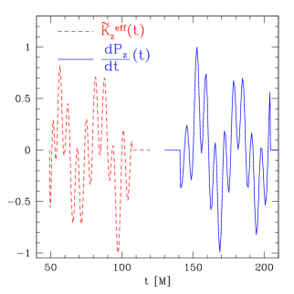
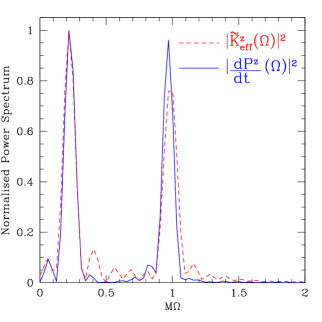
Figure 5: The left panel shows the signals $\tilde{K}^{\mathrm{eff}}_{z}(t)$ and $(dP^{\mathrm{B}}[\xi]/dt)(t)$ shown in Fig. 4, once the exponential decay has been eliminated. The right panel presents the power spectrum of the corresponding signals showing clearly the presence of two dominating frequencies $\Omega^{\mathrm{inn}}_{1,2}$ at ${\cal H}$ and $\Omega^{\mathrm{out}}_{1,2}$ at ${I}^{+}$.

we find that only two frequencies enter the dynamics in this head-on collision, $\Omega^{\mathrm{inn}}_{1}$ and $\Omega^{\mathrm{inn}}_{2}$ at ${\cal H}$ and $\Omega^{\mathrm{out}}_{1}$ and $\Omega^{\mathrm{out}}_{2}$ at ${I}^{+}$ (cf. right panel in Fig. 5). From the very good approximation Jaramillo et al. (2011a) given by $\tilde{K}^{\mathrm{eff}}_{z}\sim\tilde{\cal N}_{2}\tilde{\cal N}_{3}$ and $(dP_{z}^{\cal B}/dt)\sim{\cal N}_{2}{\cal N}_{3}$, where $\tilde{\cal N}_{\ell}$ and ${\cal N}_{\ell}$ are the ($m=0$) spherical harmonic components of $\tilde{\cal N}$ and ${\cal N}$, respectively. Remarkably, using a sinusoidal Ansatz for $\tilde{\cal N}_{\ell}$ and ${\cal N}_{\ell}$, we can reconstruct from $\Omega^{\mathrm{inn}}_{1,2}$ at ${\cal H}$ and $\Omega^{\mathrm{out}}_{1,2}$ at ${I}^{+}$, the corresponding $\ell=2$ and $\ell=3$ modes

$$\Omega^{\tilde{\cal N}}_{\ell=2}=\frac{\Omega^{\mathrm{inn}}_{2}-\Omega^{\mathrm{inn}}_{1}}{2}\,,\quad\Omega^{\tilde{\cal N}}_{\ell=3}=\frac{\Omega^{\mathrm{inn}}_{2}+\Omega^{\mathrm{inn}}_{1}}{2}\,,\quad\Omega^{\cal N}_{\ell=2}=\frac{\Omega^{\mathrm{out}}_{2}-\Omega^{\mathrm{out}}_{1}}{2}\,,\quad\Omega^{\cal N}_{\ell=3}=\frac{\Omega^{\mathrm{out}}_{2}+\Omega^{\mathrm{out}}_{1}}{2}\,,$$ (17)

leading to an extremely good agreement with the real part of the BH quasi-normal mode frequencies $\omega^{\rm R}_{\ell=2}$ and $\omega^{\rm R}_{\ell=3}$. On the other hand, the decay inverse time scales $\kappa_{\mathrm{inn}}$ and $\kappa_{\mathrm{out}}$ can be retrieved from the addition of the imaginary part of the $\ell=2$ and $\ell=3$ quasi-normal modes: $\kappa_{\mathrm{decay}}=\omega^{\rm I}_{\ell=2}+\omega^{\rm I}_{\ell=3}$. This matching of the frequencies at ${\cal H}$ and ${I}^{+}$ with the quasi-normal modes is shown in Table 1. On the one hand, this identification of the role played by the quasi-normal modes is consistent with the simple dynamics of the gravitational field in vacuum. On the other hand, it impacts directly our specific recoil dynamics problem since characteristic decay and oscillation timescales can be constructed from the imaginary and real parts, respectively, of the quasi-normal modes

$$\tau\equiv\frac{2\pi}{\omega_{\ell=2}^{\textrm{I}}+\omega_{\ell=3}^{\textrm{I}}}\,,\qquad T\equiv\frac{2\pi}{\omega_{\ell=3}^{\textrm{R}}+\omega_{\ell=2}^{\textrm{R}}}\,,$$ (18)

leading to the slowness parameter introduce in Eq. (7)

$$P\equiv\frac{T}{\tau}=\frac{\omega_{\ell=2}^{\textrm{I}}+\omega_{\ell=3}^{\textrm{I}}}{\omega_{\ell=3}^{\textrm{R}}+\omega_{\ell=2}^{\textrm{R}}}\ .$$ (19)

Table 1: The first row shows the comparison between the $\ell=2,3$ oscillation frequencies at ${\cal H}$ (i.e. $\Omega^{\tilde{\cal N}}_{\ell=2,3}$) and at ${I}^{+}$ (i.e. $\Omega^{\cal N}_{\ell=2,3}$) with the real part of quasi-normal modes of a Schwarzschild BH, $\omega^{\rm R}_{\ell=2,3}$. The second row shows the comparison between the decay exponents $\kappa_{\mathrm{inn}}$ and $\kappa_{\mathrm{out}}$, respectively at ${\cal H}$ and ${I}^{+}$, with the decay coefficient calculated from the imaginary part of the quasi-normal modes as $\kappa_{\mathrm{decay}}=\omega^{\rm I}_{\ell=2}+\omega^{\rm I}_{\ell=3}$.

$M\Omega^{\tilde{\cal N}}_{\ell=2}$	$M\Omega^{\cal N}_{\ell=2}$	$M\omega^{\rm R}_{\ell=2}$	$M\Omega^{\tilde{\cal N}}_{\ell=3}$	$M\Omega^{\cal N}_{\ell=3}$	$M\omega^{\rm R}_{\ell=3}$
$0.38\pm 0.04$	$0.37\pm 0.04$	$0.37367$	$0.60\pm 0.04$	$0.59\pm 0.04$	$0.59944$
$M\kappa_{\mathrm{inn}}$	$M\kappa_{\mathrm{out}}$	$M\kappa_{\mathrm{decay}}$
$0.181\pm 0.006$	$0.179\pm 0.005$	$0.18166$

This expression has a predictive power to estimate the recoil of the final BH remnant, from an initial configuration of binary BHs. Indeed, using analytic estimations of the final BH $M$ mass and spin parameter $a$ corresponding to given initial configurations Rezzolla (2009), one can calculate the associated Kerr quasi-normal modes and construct $P$ in (19). Further insight into this slowness parameter $P$ is gained from the dynamics of the geometry of the dynamical horizon ${\cal H}$. As shown in Eq. (12), the expansion $\theta^{(h)}$ controls the dynamical decay of the intrinsic geometry. This dissipative role of $\theta^{(h)}$ is further supported by its interpretation in the membrane paradigm Damour (1979, 1982); Price and Thorne (1986a, b); Gourgoulhon and Jaramillo (2006a); Gourgoulhon (2005); Gourgoulhon and Jaramillo (2006b, 2008) (see also discussion in Jaramillo et al. (2011b)) as associated with bulk viscosity terms, whereas $\sigma^{(h)}_{ab}$ is related to the shear viscosity. The latter is responsible for the (shape) oscillations in the intrinsic geometry (cf. last equation in (4.1), for its relation to propagating gravitational degrees of freedom encoded in the Weyl tensor). Given the physical dimensions $[\theta^{(h)}]=[\sigma^{(h)}]=[\mathrm{Length}]^{-1}$, one could introduce decay and oscillation inverse timescales by averaging $\theta^{(h)}$ and $\sigma^{(h)}$, respectively, over the horizon section ${\cal S}_{t}$. In order to make more precise this heuristic approach, we consider the evolution equation for $\theta^{(h)}$ Gourgoulhon and Jaramillo (2006b)

$$\left(\delta_{h}+\theta^{(h)}\right)\theta^{(h)} = -\kappa^{(h)}\theta^{(h)}+\sigma^{(h)}_{ab}{\sigma^{(\tau)}}^{ab}$$ (21)

$$+\frac{(\theta^{(h)})^{2}}{2}+{}^{2}\!D^{a}({}^{2}\!D_{a}C-2C\Omega^{(\ell)}_{a})+8\pi T_{ab}\tau^{a}h^{b}-\theta^{(k)}\delta_{h}C\ \ .$$

Denoting by $\xi^{i}_{t}$ the unit vector in the instantaneous spatial direction of motion of the BH, decay and oscillation timescales can be introduced as

$$\frac{1}{\tau(t)^{2}} \equiv \frac{1}{A}\oint_{{\cal S}_{t}}(\xi_{t}^{i}s_{i})\left(\kappa^{(h)}\theta^{(h)}\right)dA\$$

$$\frac{1}{T(t)^{2}} \equiv \frac{1}{A}\oint_{{\cal S}_{t}}(\xi_{t}^{i}s_{i})\left(\sigma_{ab}^{(h)}{\sigma^{(\tau)}}^{ab}\right)dA\quad,\quad$$ (22)

so that the instantaneous slowness parameter

$$P(t)=\frac{T(t)}{\tau(t)}=\left(\frac{\oint_{{\cal S}_{t}}(\xi_{t}^{i}s_{i})\left(\kappa^{(h)}\theta^{(h)}\right)dA}{\oint_{{\cal S}_{t}}(\xi_{t}^{i}s_{i})\left(\sigma_{ab}^{(h)}{\sigma^{(\tau)}}^{ab}\right)dA}\right)^{\frac{1}{2}}$$ (23)

satisfies $P(t)\approx 1$ near equilibrium, when derivative and higher-order terms in (21) can be neglected, only surviving the terms in the first line of the right-hand side, precisely those used to define $T(t)$ and $\tau(t)$ (note that they lead to the Hartle-Hawking area evolution equation). Note that $P\approx 1$ is consistent with the absence of antikick near-equilibrium.

4.2 Contact with quasi-local BH linear momentum

Quasi-local notions of linear momentum has been applied to the study of BH recoil dynamics in Krishnan et al. (2007); Lovelace et al. (2010). From this perspective, the news-like function ${\cal N}_{ab}^{\cal H}$ in Eq. (11) can be used to introduce a heuristic flux of Bondi-like momentum at the horizon ${\cal H}$. Consider the (timelike) unit normal $\hat{\tau}^{a}=\frac{\tau^{a}}{\sqrt{|\tau^{b}\tau_{b}|}}=\frac{1}{\sqrt{2C}}(\ell^{a}+Ck^{a})=\frac{1}{\sqrt{2C}}(bn^{a}+Ns^{a})$ to ${\cal H}$ (here, $n^{a}$ is the timelike unit normal to a 3-slice $\Sigma_{t}$ and $s^{a}$ is the spacelike unit normal to ${\cal S}_{t}$ in $\Sigma_{t}$). Consider also a generic 4-vector $\eta^{a}$. We can introduce a flux of Bondi-like 4-momentum as Jaramillo et al. (2011b) (note the natural use of an advanced time parameter $v$)

$$\frac{dP^{\tau}[\eta]}{dv}\equiv-\frac{1}{8\pi}\oint_{{\cal S}_{v}}(\eta^{c}\hat{\tau}_{c})\left({\cal N}^{{}^{({\cal H})}}_{ab}{\cal N}^{{}^{({\cal H})}ab}\right)dA=-\frac{1}{16\pi}\oint_{{\cal S}_{v}}(\eta^{c}\hat{\tau}_{c})\left({\sigma}^{(h)}_{ab}{\sigma^{(h)}}^{ab}\right)dA\ .$$ (24)

Considering an Eulerian observer $n^{a}$, the associated flux of energy would be

$$\frac{dE^{\tau}}{dv}(v)\equiv\frac{dP^{\tau}[n^{a}]}{dv}=\frac{1}{16\pi}\oint_{\cal S}\frac{b}{\sqrt{2C}}\left(\sigma^{(h)}_{ab}{\sigma^{(h)}}^{ab}\right)dA\ ,$$ (25)

with $\frac{b}{\sqrt{2C}}=\sqrt{1+N^{2}/2C}$, whereas the flux of Bondi-like linear momentum is given by

$$\frac{dP^{\tau}[\xi]}{dv}=-\frac{1}{16\pi}\oint_{{\cal S}_{v}}\frac{N}{\sqrt{2C}}(\xi^{i}s_{i})\left(\sigma^{(h)}_{ab}{\sigma^{(h)}}^{ab}\right)dA\ .$$ (26)

These expressions are closely related to those proposed for DHs Ashtekar and Krishnan (2002, 2003). The integration in time $v$ along the horizon ${\cal H}$ provides a heuristic prescription for the linear momentum, a sort of Bondi-like counterpart of the heuristic prescription in Eq. (8) based on the ADM momentum. More generally, for a quantity $Q(v)$ with $F(v)$ flux through ${\cal S}$, we write

$$Q(v)=Q(v_{0})+\int_{v_{0}}^{v}F(v^{\prime})dv^{\prime}\ \ .$$ (27)

Note that, in view of the 3+1 description (cf. Fig 3) such an expression can be split into

$$Q(t)=Q_{0}+\int^{t}_{t_{c}}\left(F\right)^{\mathrm{int}}(t^{\prime})dt^{\prime}+\int_{t_{c}}^{t}\left(F\right)^{\mathrm{ext}}(t^{\prime})dt^{\prime}+\mathrm{Res}(t)$$

where $\left(F\right)^{\mathrm{int}}$ is the flux through the internal horizon, $\left(F\right)^{\mathrm{ext}}$ is the flux through the external horizon and a residual $\mathrm{Res}(t)=\int^{\infty}_{t}F^{\mathrm{int}}(t^{\prime})dt^{\prime}$ must be included (a more complete expression taking into account changes in the metric type of ${\cal H}$ is discussed in Jaramillo et al. (2011b)). This expression makes explicit the relevance of tracking the internal horizon when addressing the integration in time of physical fluxes across the dynamical horizon ${\cal H}$.

5 Conclusions and perspectives

We have outlined some basic elements of a cross-correlation approach to the analysis near-horizon spacetime dynamics. In particular, we have identified DHs as hypersurfaces providing inner canonical screens in a 3+1 Initial Value Problem approach to the spacetime construction, where appropriate geometric quantities can be defined to probe and monitor bulk dynamics, namely through correlation with quantities at an outer screen.

We have applied this scheme to the study of BH recoil dynamics. First, we have introduced a heuristic horizon news-like function to build a quantity $dP^{{}^{({\cal H})}}[\xi]/dv$ tracking quasi-locally (on ${\cal H}$) the qualitative and to a good extent also the quantitative features of the recoil dynamics at ${I}^{+}$. In particular, the analysis of its correlations with the flux of Bondi momentum at ${I}^{+}$ in numerically constructed spacetimes corresponding to binary BH head-on collisions confirms the simple character of vacuum spacetime dynamics in this setting. Second, this latter remark has led to the proposal of a prescription for a slowness parameter $P$, as constructed from the complex BH quasi-normal modes. More generally, inspired by the BH horizon viscous fluid analogy in the membrane paradigm and further supported by the horizon geometry dynamics, we have proposed geometric decay and oscillation timescales leading to a more general characterization of the slowness parameter $P$, with a well-defined instantaneous meaning. Third, we have made contact with the heuristic attempts for estimating the BH 4-momentum, with the proposal of a quasi-local Bondi-like expression. In this context, we have emphasized the relevance of the internal 3+1 horizon when considering flux integrations along the BH horizon ${\cal H}$. An open problem in this sense is to assess the capability of a DH to dress the BH singularity, this involving the understanding of early and late DH asymptotics.

Despite the encouraging prospects, there are important caveats in the sketched cross-correlation approach. First, a sound proper formalism is missing. In particular, an “inverse scattering” picture must still be systematically developed. In addition, the gauge issue briefly referred to as the “time stretch issue” must be addressed in generic situations. More importantly, it is not clear how to assess the conditions under which the comparison/cross-correlation of quantities at outer and inner screens is actually legitimate. A possible approach to these issues (cf. Jaramillo (2011)) would consist in considering the cross-correlation of test-fields evolving on dynamical spacetimes, without backreacting on them, so that the field evolution faithfully tracks specific relevant aspects in the geometry of the spacetime dynamics (see also Bentivegna et al. (2008)). On the one hand, this would remove the ambiguities in the choice of quantities $h_{\mathrm{inn}}$ and $h_{\mathrm{out}}$ to be correlated at ${\cal H}_{\mathrm{inn}}$ and ${\cal H}_{\mathrm{out}}$. On the other hand, it would permit to extend the scheme to the direct analysis of bulk quantities (this would be related to the techniques in Owen et al. (2011); Nichols et al. (2011) for tracking spacetime dynamics). In particular, the strategy of analyzing the spacetime geometry in terms of correlations of appropriate test-fields, that could be paraphrased as pouring sand on a transparent surface, can benefit from the use of tools and concepts developed in statistical approaches to field theory in curved spacetimes, e.g. Calzetta et al. (1988); Hu (1989); Calzetta and Hu (1994, 1995); Hu (1996); Calzetta and Hu (2000); Hu and Verdaguer (2008). This attempt leads to the following declaration of intentions as a perspective for future: to develop a strategy for spacetime analysis aiming at a functional and coarse-grained description of the spacetime geometry, by importing functional tools for the analysis of condensed matter and quantum/statistical field theory systems (in curved backgrounds).

References

- Penrose (1973) R. Penrose, Annals N. Y. Acad. Sci. 224, 125 (1973).
- Penrose (1965) R. Penrose, Phys. Rev. Lett. 14, 57 (1965).
- Hawking (1967) S. Hawking, Proc. R. Soc. London, Ser. A 300, 182 (1967).
- Hawking and Penrose (1970) S. Hawking, and R. Penrose, Proc. R. Soc. London, Ser. A 314, 529–548 (1970).
- Hawking and Ellis (1973) S. W. Hawking, and G. F. R. Ellis, The large scale structure of space-time, Cambridge University Press, 1973.
- Penrose (1969) R. Penrose, Riv. Nuovo Cim. 1, 252 (1969).
- Heusler (1998) M. Heusler, Liv. Rev. Relat. 1, 6 (1998).
- Jaramillo et al. (2011a) J. L. Jaramillo, R. P. Macedo, P. Moesta, and L. Rezzolla, to appear in Phys. Rev. D (2011a), 1108.0060.
- Jaramillo et al. (2011b) J. L. Jaramillo, R. P. Macedo, o. P. Moesta, and L. Rezzolla, to appear in Phys. Rev. D (2011b), 1108.0061.
- Jaramillo (2011) J. L. Jaramillo (2011), 1108.2408.
- Hayward (1994) S. Hayward, Phys. Rev. D 49, 6467 (1994).
- Andersson et al. (2005) L. Andersson, M. Mars, and W. Simon, Phys. Rev. Lett. 95, 111102 (2005).
- Andersson et al. (2008) L. Andersson, M. Mars, and W. Simon, Adv. Theor. Math. Phys. 12, 853–888 (2008).
- Booth and Fairhurst (2007) I. Booth, and S. Fairhurst, Phys. Rev. D75, 084019 (2007), gr-qc/0610032.
- Ashtekar and Krishnan (2004) A. Ashtekar, and B. Krishnan, Liv. Rev. Relat. 7, 10 (2004).
- Gourgoulhon and Jaramillo (2006a) E. Gourgoulhon, and J. L. Jaramillo, Phys. Rept. 423, 159 (2006a).
- Ashtekar and Krishnan (2002) A. Ashtekar, and B. Krishnan, Phys. Rev. Lett. 89, 261101 (2002).
- Ashtekar and Krishnan (2003) A. Ashtekar, and B. Krishnan, Phys. Rev. D 68, 104030 (2003).
- Ashtekar and Galloway (2005) A. Ashtekar, and G. J. Galloway, Adv. Theor. Math. Phys. 9, 1 (2005), gr-qc/0503109.
- Bengtsson and Senovilla (2011) I. Bengtsson, and J. M. Senovilla, Phys.Rev. D83, 044012 (2011), 1009.0225.
- Sperhake et al. (2011) U. Sperhake, E. Berti, V. Cardoso, F. Pretorius, and N. Yunes, Phys. Rev. D 83, 024037 (2011), 1011.3281.
- Price et al. (2011) R. H. Price, G. Khanna, and S. A. Hughes, Phys.Rev. D83, 124002 (2011), 1104.0387.
- Rezzolla et al. (2010) L. Rezzolla, R. P. Macedo, and J. L. Jaramillo, Phys. Rev. Lett. 104, 221101 (2010), 1003.0873.
- Krishnan et al. (2007) B. Krishnan, C. O. Lousto, and Y. Zlochower, Phys. Rev. D76, 081501 (2007), arXiv:0707.0876[gr-qc].
- Rezzolla (2009) L. Rezzolla, Class. Quant. Grav. 26, 094023 (2009), 0812.2325.
- Damour (1979) T. Damour, Quelques propriétés mécaniques, électromagnétiques, thermodynamiques et quantiques des trous noirs, Thèse de doctorat d’ tat, Université Paris 6, 1979.
- Damour (1982) T. Damour, “Surface effects in black hole physics,” in Proceedings of the Second Marcel Grossmann Meeting on General Relativity, edited by R. Ruffini, North-Holland, Amsterdam, 1982, p. 587.
- Price and Thorne (1986a) R. H. Price, and K. S. Thorne, Phys. Rev. D33, 915 (1986a).
- Price and Thorne (1986b) R. H. Price, and K. S. Thorne, Phys. Rev. D 33, 915 (1986b).
- Gourgoulhon (2005) E. Gourgoulhon, Phys. Rev. D72, 104007 (2005), gr-qc/0508003.
- Gourgoulhon and Jaramillo (2006b) E. Gourgoulhon, and J. L. Jaramillo, Phys. Rev. D74, 087502 (2006b), gr-qc/0607050.
- Gourgoulhon and Jaramillo (2008) E. Gourgoulhon, and J. L. Jaramillo, New Astron. Rev. 51, 791–798 (2008), 0803.2944.
- Lovelace et al. (2010) G. Lovelace, et al., Phys. Rev. D 82, 064031 (2010), 0907.0869.
- Bentivegna et al. (2008) E. Bentivegna, D. M. Shoemaker, I. Hinder, and F. Herrmann, Phys.Rev. D77, 124016 (2008), 0801.3478.
- Owen et al. (2011) R. Owen, J. Brink, Y. Chen, J. D. Kaplan, G. Lovelace, K. D. Matthews, D. A. Nichols, M. A. Scheel, F. Zhang, A. Zimmerman, and K. S. Thorne, Phys. Rev. Lett. 106, 151101 (2011).
- Nichols et al. (2011) D. A. Nichols, R. Owen, F. Zhang, A. Zimmerman, J. Brink, et al., Phys.Rev. D84, 124014 (2011), 25 pages, 20 figures, matches the published version, 1108.5486.
- Calzetta et al. (1988) E. Calzetta, S. Habib, and B. Hu, Phys.Rev. D37, 2901 (1988).
- Hu (1989) B. Hu, Physica A158, 399–424 (1989).
- Calzetta and Hu (1994) E. Calzetta, and B. Hu, Phys.Rev. D49, 6636–6655 (1994), gr-qc/9312036.
- Calzetta and Hu (1995) E. Calzetta, and B. Hu (1995), hep-th/9501040.
- Hu (1996) B. Hu (1996), gr-qc/9607070.
- Calzetta and Hu (2000) E. Calzetta, and B. Hu, Phys.Rev. D61, 025012 (2000), hep-ph/9903291.
- Hu and Verdaguer (2008) B. Hu, and E. Verdaguer, Living Rev.Rel. 11, 3 (2008), 0802.0658.