Variational Inference for Generalized Linear Mixed Models Using Partially Noncentered Parametrizations

Abstract

The effects of different parametrizations on the convergence of Bayesian computational algorithms for hierarchical models are well explored. Techniques such as centering, noncentering and partial noncentering can be used to accelerate convergence in MCMC and EM algorithms but are still not well studied for variational Bayes (VB) methods. As a fast deterministic approach to posterior approximation, VB is attracting increasing interest due to its suitability for large high-dimensional data. Use of different parametrizations for VB has not only computational but also statistical implications, as different parametrizations are associated with different factorized posterior approximations. We examine the use of partially noncentered parametrizations in VB for generalized linear mixed models (GLMMs). Our paper makes four contributions. First, we show how to implement an algorithm called nonconjugate variational message passing for GLMMs. Second, we show that the partially noncentered parametrization can adapt to the quantity of information in the data and determine a parametrization close to optimal. Third, we show that partial noncentering can accelerate convergence and produce more accurate posterior approximations than centering or noncentering. Finally, we demonstrate how the variational lower bound, produced as part of the computation, can be useful for model selection.

abstractwidth360pt keywordwidth360pt

and

1 Introduction

The convergence of Markov chain Monte Carlo (MCMC) algorithms depends greatly on the choice of parametrization and simple reparametrizations can often give improved convergence. Here we investigate the use of centered, noncentered and partially noncentered parametrizations of hierarchical models in the context of variational Bayes (VB) (Attias (1999)). As a fast deterministic approach to approximation of the posterior distribution in Bayesian inference, VB is attracting increasing interest due to its suitability for large high-dimensional data (see, e.g., Braun and McAuliffe (2010); Hoffman et al. (2012)). VB methods approximate the intractable posterior by a factorized distribution which can be represented by a directed graph and optimization of the factorized variational posterior can be decomposed into local computations that involve only neighboring nodes. Variational message passing(Winn and Bishop (2005)) is an algorithmic implementation of VB that can be applied to a general class of conjugate-exponential models (Attias (2000); Ghahramani and Beal (2001)). Knowles and Minka (2011) proposed an algorithm called a nonconjugate variational message passing to extend variational message passing to nonconjugate models.

We examine the use of partially noncentered parametrization in VB for generalized linear mixed models (GLMMs). Our paper makes four contributions. First, we show how to implement nonconjugate variational message passing for GLMMs. Second, we show that the partially noncentered parametrization is able to adapt to the quantity of information in the data so that it is not necessary to make a choice in advance between centering and noncentering with the data deciding the optimal parametrization. Third, we show that in addition to accelerating convergence, partial noncentering is a good strategy statistically for VB in terms of producing more accurate approximations to the posterior than either centering or noncentering. Finally, we demonstrate how the variational lower bound, which is produced as part of the computation, can be useful for model selection.

GLMMs extend generalized linear models by the inclusion of random effects to account for correlation of observations in grouped data and are of wide applicability. Estimation of GLMMs using maximum likelihood is challenging, as the integral over random effects is intractable. Methods involving numerical quadrature or MCMC to approximate these integrals are computationally intensive. Various approximate methods such as penalized quasi-likelihood (Breslow and Clayton (1993)), Laplace approximation and its extension (Raudenbush, Yang and Yosef (2000)) and Gaussian variational approximation(Ormerod and Wand (2012)) have been developed. Fong, Rue and Wakefield (2010) considered a Bayesian approach using integrated nested Laplace approximations. We show how to fit GLMMs using nonconjugate variational message passing, focusing on Poisson and logistic mixed models and their applications in longitudinal data analysis.

The literature on parametrization of hierarchical models including partial noncentering techniques for accelerating MCMC algorithms is inspired by earlier similar work for the expectation maximization (EM) algorithm (see Meng and van Dyk, 1997, 1999; Liu and Wu (1999)). Gelfand, Sahu and Carlin (1995, 1996) proposed hierarchical centering for normal linear mixed models and GLMMs to improve the slow mixing in MCMC algorithms due to high correlations between model parameters. Papaspiliopoulos, Roberts and Sköld (2003, 2007) demonstrated that centering and noncentering play complementaryroles in boosting MCMC efficiency and neither are uniformly effective. They considered the partially noncentered parametrization which is data dependent and lies on the continuum between the centered and noncentered parametrizations. Extending this idea, Christensen, Roberts and Sköld (2006) devised reparametrization techniques to improve performance for Hastings-within Gibbs algorithms for spatialGLMMs. Yu and Meng (2011) introduced a strategy for boosting MCMC efficiency via interweaving the centered and noncentered parametrizations to reduce dependence between draws. Parameter-expanded VB methods were proposed by Qi and Jaakkola (2006) to reduce coupling in updates and speed up VB.

The idea of partial noncentering is to introduce a tuning parameter via reparametrization of the model and then seek its optimal value for fastest convergence. For the normal hierarchical model, Papaspiliopoulos, Roberts and Sköld (2003) showed that the partially noncentered parametrization has convergence properties superior to that of the centered and noncentered parametrizations for the Gibbs sampler. As the rate of convergence of an algorithm based on VB is equal to that of the corresponding Gibbs sampler when the target distribution is Gaussian (Tan and Nott (2013)), partial noncentering will similarly outperform centering and noncentering in the context of VB for the normal hierarchical model. This provides motivation to consider partial noncentering in the VB context. We illustrate this idea with the following example.

Initialize $\mu_{\tilde{\alpha}_{i}}^{q}$ and $\Sigma_{\tilde{\alpha}_{i}}^{q}$ for $i=1,\ldots,n$.

Cycle:

Cycle:$\Sigma_{\beta}^{q}\leftarrow[\sum_{i=1}^{n}\{(I-W_{i})^{T}D^{-1}(I-W_{i})+\frac{1}{\sigma^{2}}W_{i}^{T}X_{i}^{T}X_{i}W_{i}\}]^{-1}$

Cycle:$\mu_{\beta}^{q}\leftarrow\Sigma_{\beta}^{q}\sum_{i=1}^{n}[\frac{1}{\sigma^{2}}W_{i}^{T}X_{i}^{T}y_{i}+\{D^{-1}(I-W_{i})-\frac{1}{\sigma^{2}}X_{i}^{T}X_{i}W_{i}\}^{T}\mu_{\tilde{\alpha}_{i}}^{q}]$

Cycle:For $i=1,\ldots,n$,

Cycle:For $\Sigma_{\tilde{\alpha}_{i}}^{q}\leftarrow(D^{-1}+\frac{1}{\sigma^{2}}X_{i}^{T}X_{i})^{-1}$

Cycle:For $\mu_{\tilde{\alpha}_{i}}^{q}\leftarrow\Sigma_{\tilde{\alpha}_{i}}^{q}[\frac{1}{\sigma^{2}}X_{i}^{T}y_{i}+\{D^{-1}(I-W_{i})-\frac{1}{\sigma^{2}}X_{i}^{T}X_{i}W_{i}\}\mu_{\beta}^{q}]$

until convergence.

Algorithm 1: Iterative scheme for obtaining variational parameters in linear mixed model.

1.1 Motivating Example: Linear Mixed Model

Consider the linear mixed model

$$y_{i}=X_{i}\beta+X_{i}u_{i}+\varepsilon_{i},$$ (2)

$$\eqntext{\varepsilon_{i}\sim N\bigl{(}0,\sigma^{2}I\bigr{)},i=1,\ldots,n,}$$

where $y_{i}$ is a vector of length $n_{i}$, $\beta$ is a vector of length $r$ of fixed effects, $X_{i}$ is a $n_{i}\times r$ matrix of covariates and $u_{i}$ is a vector of length $r$ of random effects independently distributed as $N(0,D)$. For simplicity, we specify a constant prior on $\beta$ and assume $\sigma^{2}$ and $D$ are known. Let

$$\alpha_{i}=\beta+u_{i}\quad\mbox{and}\quad\tilde{\alpha}_{i}=\alpha_{i}-W_{i}\beta,\quad i=1,\ldots,n,$$

where $W_{i}$ is an $r\times r$ tuning matrix to be specified. $W_{i}=0$ corresponds to the centered and $W_{i}=I$ to the noncentered parametrization. For each $i=1,\ldots,n$,

$$y_{i}=X_{i}W_{i}\beta+X_{i}\tilde{\alpha}_{i}+\varepsilon_{i}$$

and

$$\tilde{\alpha}_{i}\sim N\bigl{(}(I-W_{i})\beta,D\bigr{)}.$$

This is the partially noncentered parametrization and the set of unknown parameters is $\theta=\{\beta,\tilde{\alpha}\}$, where $\tilde{\alpha}=[\tilde{\alpha}_{1}^{T},\ldots,\tilde{\alpha}_{n}^{T}]^{T}$. Let $y=[y_{1},\ldots,y_{n}]^{T}$ denote the observed data. Of interest is the posterior distribution of $\theta$, $p(\theta|y)$.

Suppose $p(\theta|y)$ is not analytically tractable. In the variational approach, we approximate $p(\theta|y)$ by a $q(\theta)$ for which inference is more tractable and $q(\theta)$ is chosen to minimize the Kullback–Leibler divergence between $q(\theta)$ and $p(\theta|y)$ given by

$$\int q(\theta)\log\frac{q(\theta)}{p(\theta|y)}\,\mathrm{d}\theta = \int q(\theta)\log\frac{q(\theta)}{p(y,\theta)}\,\mathrm{d}\theta$$

$${}+\log p(y),$$

where $p(y)$ is the marginal likelihood $p(y)=\int p(y|\allowbreak\theta)p(\theta)\,\mathrm{d}\theta$. Since the Kullback–Leibler divergence is nonnegative,

$$\log p(y) \geq \int\log\frac{p(y,\theta)}{q(\theta)}q(\theta)\,\mathrm{d}\theta$$

$$= E_{q}\bigl{\{}\log p(y,\theta)\bigr{\}}-E_{q}\bigl{\{}\log q(\theta)\bigr{\}}$$

$$= \mathcal{L},$$

where $\mathcal{L}$ is a lower bound on the log marginal likelihood. Maximization of $\mathcal{L}$ is equivalent to minimization of the Kullback–Leibler divergence between $q(\theta)$ and $p(\theta|y)$. In VB, $q(\theta)$ is assumed to be of a factorized form, say, $q(\theta)=\prod_{i=1}^{m}q_{i}(\theta_{i})$ for some partition $\{\theta_{1},\ldots,\theta_{m}\}$ of $\theta$. Maximization of $\mathcal{L}$ over each of $q_{1},\ldots,q_{m}$ lead to optimal densities satisfying $q_{i}(\theta_{i})\propto\exp\{E_{-\theta_{i}}\log p(y,\theta)\}$, $i=1,\ldots,m$, where $E_{-\theta_{i}}$ denotes expectation with respect to the density$\prod_{j\neq i}q_{j}(\theta_{j})$. See Ormerod and Wand (2010) for an explanation of variational approximation methods very accessible to statisticians.

If we apply VB to (2) and approximate the posterior $p(\theta|y)$ with $q(\theta)=q(\beta)q(\tilde{\alpha})$, the optimal densities can be derived to be $q(\beta)=N(\mu_{\beta}^{q},\Sigma_{\beta}^{q})$ and $q(\tilde{\alpha})=\prod_{i=1}^{n}q(\tilde{\alpha}_{i})$, where $q(\tilde{\alpha}_{i})=N(\mu_{\tilde{\alpha}_{i}}^{q},\Sigma_{\tilde{\alpha}_{i}}^{q})$. The expressions for the variational parameters $\mu_{\beta}^{q}$, $\Sigma_{\beta}^{q}$ and $\mu_{\tilde{\alpha}_{i}}^{q}$, $\Sigma_{\tilde{\alpha}_{i}}^{q}$, $i=1,\ldots,m$, are, however, dependent on each other and can be computed by an iterative scheme such as that given in Algorithm 1.

Observe that Algorithm 1 converges in one iteration if $D^{-1}(I-W_{i})=\frac{1}{\sigma^{2}}X_{i}^{T}X_{i}W_{i}$ for each $i$, that is, if

$$W_{i}=\biggl{(}\frac{1}{\sigma^{2}}X_{i}^{T}X_{i}+D^{-1}\biggr{)}^{-1}D^{-1}$$ (5)

$$\eqntext{\mbox{for }i=1,\ldots,n.}$$

For this specification of the tuning parameters, partial noncentering gives more rapid convergence than centering or noncentering. Moreover, it can be shown that the true posteriors are recovered in this partially noncentered parametrization so that a better fit is achieved than in the centered or noncentered parametrizations. This example suggests that with careful tuning of $W_{i}$, $i=1,\ldots,n$, the partially noncentered parametrization can potentially outperform the centered and noncentered parametrizations in the VB context.

The rest of the paper is organized as follows. Section 2 specifies the GLMM and priors used. Section 3 describes the partially noncentered parametrization for GLMMs. Section 4 describes the nonconjugate variational message passing algorithm for fittingGLMMs. Section 5 discusses briefly the use of the variational lower bound for model selection and Section 6 considers examples including real and simulated data. Section 7 concludes.

2 The Generalized Linear Mixed Model

Consider clustered data where $y_{ij}$ denotes the $j$th response from cluster $i$, $i=1,\ldots,n$, $j=1,\ldots,n_{i}$. Conditional on the $r$-dimensional random effects $u_{i}$ drawn independently from $N(0,D)$, $y_{ij}$ is independently distributed from some exponential family distribution with density

$$\quad f(y_{ij}|u_{i})=\exp\biggl{\{}\frac{y_{ij}\zeta_{ij}-b(\zeta_{ij})}{a(\phi)}+c(y_{ij},\phi)\biggr{\}},$$ (6)

where $\zeta_{ij}$ is the canonical parameter, $\phi$ is the dispersion parameter, and $a(\cdot)$, $b(\cdot)$ and $c(\cdot)$ are functions specific to the family. The conditional mean of $y_{ij}$, $\mu_{ij}=E(y_{ij}|u_{i})$, is assumed to depend on the fixed and random effects through the linear predictor,

$$\eta_{ij}={X_{ij}^{R}}^{T}\beta^{R}+{X_{ij}^{G}}^{T}\beta^{G}+{X_{ij}^{R}}^{T}u_{i}$$

with $g(\mu_{ij})=\eta_{ij}$ for some known link function, $g(\cdot)$. Here, $X_{ij}^{R}$ and $X_{ij}=[{X_{ij}^{R}}^{T},{X_{ij}^{G}}^{T}]^{T}$ are $r\times 1$ and $p\times 1$ vectors of covariates and $\beta=[{\beta^{R}}^{T},{\beta^{G}}^{T}]^{T}$ is a $p\times 1$ vector of fixed effects. We considered the above breakdown (see Zhao et al. (2006)) for the linear predictor to allow for centering. For the $i$th cluster, let $y_{i}=[y_{i1},\ldots,y_{in_{i}}]^{T}$, $X_{i}^{R}=[X_{i1}^{R},\ldots,X_{in_{i}}^{R}]^{T}$, $X_{i}^{G}=[X_{i1}^{G},\ldots,X_{in_{i}}^{G}]^{T}$, $X_{i}=[X_{i1},\ldots,X_{in_{i}}]^{T}$ and $\eta_{i}=[\eta_{i1},\break\ldots,\eta_{in_{i}}]^{T}$. Let $1_{n_{i}}$ denote the ${n_{i}}\times 1$ column vector with all entries equal to 1. We assume that the first column of $X_{i}^{R}$ is $1_{n_{i}}$ if $X_{i}^{R}$ is not a zero matrix. For Bayesian inference, we specify prior distributions on the fixed effects $\beta$ and random effects covariance matrix $D$. In this paper, we focus on responses from the Bernoulli and Poisson families and the dispersion parameter is one in these cases, so we do not consider a prior for $\phi$. We assume a diffuse prior, $N(0,\Sigma_{\beta})$, for $\beta$ and an independent inverse Wishart prior, $\mathit{IW}(\nu,S)$, for $D$. Following the suggestion by Kass and Natarajan (2006), we set $\nu=r$ and let the scale matrix $S$ be determined from first-stage data variability. In particular, $S=r\hat{R}$, where

$$\hat{R}=c\Biggl{(}\frac{1}{n}\sum_{i=1}^{n}{X_{i}^{R}}^{T}M_{i}(\hat{\beta})X_{i}^{R}\Biggr{)}^{-1},$$ (7)

$M_{i}(\hat{\beta})$ denotes the $n_{i}\times n_{i}$ diagonal generalized linear model weight matrix with diagonal elements $[\phi v(\hat{\mu}_{ij})\cdot g^{\prime}(\hat{\mu}_{ij})^{2}]^{-1}$, $v(\cdot)$ is the variance function based on $f(\cdot)$ in (6) and $g(\cdot)$ is the link function. Here, $\hat{\mu}_{ij}=g^{-1}(X_{ij}^{T}\hat{\beta}+{X_{ij}^{R}}^{T}\hat{u}_{i})$, where $\hat{u}_{i}$ is set as $0$ for all $i$ and $\hat{\beta}$ is an estimate of the regression coefficients from the generalized linear model obtained by pooling all data and setting $u_{i}=0$ for all $i$. The value of $c$ is an inflation factor representing the amount by which within-cluster variability should be increased in determining $\hat{R}$. We used $c=1$ in all examples.

3 A Partially Noncentered Parametrization for the Generalized Linear Mixed Model

We introduce the following partially noncentered parametrization for the GLMM. For each $i=1,\ldots,n$, the linear predictor is $\eta_{i}=X_{i}^{R}\beta^{R}+X_{i}^{G}\beta^{G}+X_{i}^{R}u_{i}$. Let

$$X_{i}^{G}\beta^{G} = X_{i}^{G_{1}}\beta^{G_{1}}+X_{i}^{G_{2}}\beta^{G_{2}}$$

$$= 1_{n_{i}}{x_{i}^{G_{1}}}^{T}\beta^{G_{1}}+X_{i}^{G_{2}}\beta^{G_{2}},$$

where $\beta^{G_{1}}$ is a vector of length $g_{1}$ consisting of all parameters corresponding to subject specific covariates (i.e., the rows of $X_{i}^{G_{1}}$ are all the same and equal to the vector $x_{i}^{G_{1}}$ say). Recall that the first column of $X_{i}^{R}$ is $1_{n_{i}}$ if $X_{i}^{R}$ is not a zero matrix. We have

$$\eta_{i}=X_{i}^{R}\bigl{(}C_{i}\beta^{RG_{1}}+u_{i}\bigr{)}+X_{i}^{G_{2}}\beta^{G_{2}},$$

where

$$C_{i}=\left[\matrix{&{x_{i}^{G_{1}}}^{T}\cr I_{r}&\cr&0}\right]\quad\mbox{and}\quad\beta^{RG_{1}}=\left[\matrix{\beta^{R}\cr\beta^{G_{1}}}\right].$$

Let $\alpha_{i}=C_{i}\beta^{RG_{1}}+u_{i}$ and $\tilde{\alpha}_{i}=\alpha_{i}-W_{i}C_{i}\beta^{RG_{1}}$, where $W_{i}$ is an $r\times r$ matrix to be specified. The proportion of $C_{i}\beta^{RG_{1}}$ subtracted from each $\alpha_{i}$ is allowed to vary with $i$ as in Papaspiliopoulos, Roberts and Sköld (2003) to reflect the varying informativity of each response $y_{i}$ about the underlying $\alpha_{i}$. $W_{i}=0$ corresponds to the centered and $W_{i}=I$ to the noncentered parametrization. Finally,

$$\eta_{i} = X_{i}^{R}\bigl{(}\tilde{\alpha}_{i}+W_{i}C_{i}\beta^{RG_{1}}\bigr{)}+X_{i}^{G_{2}}\beta^{G_{2}}$$

$$= V_{i}\beta+X_{i}^{R}\tilde{\alpha}_{i},$$

where $V_{i}=[X_{i}^{R}W_{i}C_{i}\enskip X_{i}^{G_{2}}]$ and $\tilde{\alpha}_{i}\sim N((I-W_{i})\cdot C_{i}\beta^{RG_{1}},D)$. We refer to (3) as the partially noncentered parametrization. Let $\tilde{\alpha}=[\tilde{\alpha}_{1}^{T},\ldots,\tilde{\alpha}_{n}^{T}]^{T}$ and $\theta=\{\beta,D,\tilde{\alpha}\}$ denote the set of unknown parameters in the GLMM. The joint distribution of $p(y,\theta)$ is

$$p(y,\theta) = \Biggl{\{}\prod_{i=1}^{n}p(y_{i}|\beta,\tilde{\alpha}_{i})p(\tilde{\alpha}_{i}|\beta,D)\Biggr{\}}$$

$${}\cdot p(\beta|\Sigma_{\beta})p(D|\nu,S).$$

Figure 1 shows the factor graph for $p(y,\theta)$ where there is a node (circle) for every variable, which is shaded in the case of observed variables, and a node (filled rectangle) for each factor in the joint distribution. Constants or hyperparameters are denoted with smaller filled circles. Each factor node is connected by undirected links to all of the variable nodes on which that factor depends (see Bishop (2006)).

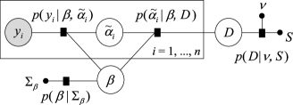
Figure 1: Factor graph for $p(y,\theta)$ in (3). Filled rectangles denote factors and circles denote variables (shaded for observed variables). Smaller filled circles denote constants or hyperparameters. The box represents a plate which contains variables and factors to be replicated. Number of repetitions is indicated in the lower right corner.

Next, we consider specification of the tuning parameter $W_{i}$, referring to the linear mixed model example in Section 1.1 which is a special case of the GLMM in (6) with an identity link.

3.1 Specification of Tuning Parameter

It is interesting to note that for the linear mixed model in (2), the expression for $W_{i}$ leading to optimal performance in VB and the Gibbs sampling algorithm is exactly the same (see Papaspiliopoulos, Roberts and Sköld, 2003). Gelfand, Sahu and Carlin (1995) also observed the importance of $W_{i}$ in assessing convergence properties of the centered parametrization. They showed that $|W_{i}|<1$ for all $i$ and $|W_{i}|$ is close to zero (centering is more efficient) when the generalized variance $|D|$ is large. On the other hand, $|W_{i}|$ is close to 1 (noncentering works better) when the error variance is large. Outside the Gaussian context, Papaspiliopoulos, Roberts andSköld (2003) considered partial noncentering for the spatial GLMM and specified the tuning parameters by using a quadratic expansion of the log-likelihood to obtain an indication of the information present in $y_{i}$. Observe that $W_{i}$ in (5) can be expressed as

$$W_{i}=\bigl{(}\mathcal{I}_{f}+D^{-1}\bigr{)}^{-1}D^{-1},$$ (10)

if $\ell=\log p(y_{i}|\beta,\alpha_{i})$ denotes the log-likelihood and $\mathcal{I}_{f}=-\frac{\partial^{2}\ell}{\partial{\alpha}_{i}\,\partial{\alpha}_{i}^{T}}$. We use (10) to extend partially noncentered parametrizations to GLMMs and consider the specification of $W_{i}$ for responses from the Bernoulli and Poisson families in particular.

Recall that the linear predictor $\eta_{i}$ can be expressed as $X_{i}^{R}\alpha_{i}+X_{i}^{G_{2}}\beta^{G_{2}}$. For Poisson responses with the log link function, we allow for an offset $\log E_{ij}$ so that $\log\mu_{ij}=\log E_{ij}+\eta_{ij}$. Let $E_{i}=[E_{i1},\ldots,E_{in_{i}}]^{T}$. We have

$$\qquad\ell = y_{i}^{T}(\log E_{i}+\eta_{i})-E_{i}^{T}\exp(\eta_{i})$$ (11)

$${}-1_{n_{i}}^{T}\log(y_{i}!)\quad\mbox{and}$$

$$\mathcal{I}_{f} = \sum_{j=1}^{n_{i}}E_{ij}\exp(\eta_{ij}){X_{ij}^{R}}{X_{ij}^{R}}^{T}\approx\sum_{j=1}^{n_{i}}y_{ij}{X_{ij}^{R}}{X_{ij}^{R}}^{T},$$

if we approximate the conditional mean $\mu_{ij}$ with the response. For Bernoulli responses with the logit link function, we have

$$\ell = y_{i}^{T}\eta_{i}-1_{n_{i}}^{T}\log\bigl{\{}1_{n_{i}}+\exp(\eta_{i})\bigr{\}}\quad\mbox{and}$$

$$\mathcal{I}_{f} = \sum_{j=1}^{n_{i}}\frac{\exp(\eta_{ij})}{\{1+\exp(\eta_{ij})\}^{2}}{X_{ij}^{R}}{X_{ij}^{R}}^{T}.$$

The specification of $W_{i}$ depends on the random effects covariance $D$ and, for Bernoulli responses, on the linear predictor $\eta_{i}$ as well. In Algorithm 3, we initialize $W_{i}$ by considering $\eta_{i}=X_{i}\beta+X_{i}^{R}u_{i}$ and using estimates of $D$, $\beta$ and $u_{i}$ from penalized quasi-likelihood. Subsequently, we can either keep $W_{i}$ as fixed or update them by replacing $D$ with $\frac{S^{q}}{\nu^{q}-r-1}$, assuming the variational posterior of $D$ is $\mathit{IW}(\nu^{q},S^{q})$ and $\eta_{i}$ with $V_{i}\mu_{\beta}^{q}+X_{i}^{R}\mu_{\tilde{\alpha}_{i}}^{q}$, where $\mu_{\beta}^{q}$ and $\mu_{\tilde{\alpha}_{i}}^{q}$ are the variational posterior means of $\beta$ and $\tilde{\alpha}_{i}$, respectively. This can be done at the beginning of each iteration after new estimates of $\mu_{\beta}^{q}$, $\mu_{\tilde{\alpha}_{i}}^{q}$, $\nu^{q}$ and $S^{q}$ are obtained (see Algorithm 3 step 1).

4 Variational Inference for GLMMs

In this section we present the nonconjugate variational message passing algorithm recently developed in machine learning by Knowles and Minka (2011) for fitting GLMMs. Recall that in VB, the posterior distribution $p(\theta|y)$ is approximated by a $q(\theta)$ which is assumed to be of a factorized form, say, $q(\theta)=\prod_{i=1}^{m}q_{i}(\theta_{i})$ for some partition $\{\theta_{1},\ldots,\theta_{m}\}$ of $\theta$. For conjugate-exponential models, the optimal densities $q_{i}$ will have the same form as the prior so that it suffices to update the parameters of $q_{i}$, such as in Algorithm 1. Variational message passing (Winn and Bishop (2005)) is an algorithm which allows VB to be applied to conjugate-exponential models without having to derive application-specific updates. In the case of GLMMs where the responses are from the Bernoulli or Poisson families, the factor $p(y_{i}|\beta,\tilde{\alpha}_{i})$ of $p(y,\theta)$ in (3) is nonconjugate with respect to the prior distributions over $\beta$ and $\tilde{\alpha}_{i}$ for each $i=1,\ldots,n$. Therefore, if we apply VB and assume, say, $q(\theta)=q(\beta)q(D)\prod_{i=1}^{n}q(\tilde{\alpha}_{i})$, the optimal densities for $q(\beta)$ and $q(\tilde{\alpha}_{i})$ will not belong to recognizable density families.

4.1 Nonconjugate Variational Message Passing

In nonconjugate variational message passing, besides assuming that $q(\theta)$ must factorize into$\prod_{i=1}^{m}q_{i}(\theta_{i})$ for some partition $\{\theta_{1},\ldots,\theta_{m}\}$ of $\theta$, we impose another restriction that each $q_{i}$ must belong to some exponential family. In this way, we only have to find the parameters of each $q_{i}$ that maximizes the lower bound $\mathcal{L}$. Suppose each $q_{i}$ can be written in the form

$$q_{i}(\theta_{i})=\exp\bigl{\{}\lambda_{i}^{T}t(\theta_{i})-h(\lambda_{i})\bigr{\}},$$

where $\lambda_{i}$ is the vector of natural parameters and $t(\cdot)$ are the sufficient statistics. We wish to maximize $\mathcal{L}$ with respect to the variational parameters $\lambda_{1},\ldots,\lambda_{m}$ which are also natural parameters of$q_{1}(\theta_{1}),\ldots,q_{m}(\theta_{m})$, respectively. In the following, we show that nonconjugate variational message passing can be interpreted as a fixed-point iteration where updates are obtained from the condition that the gradient of $\mathcal{L}$ with respect to each $\lambda_{i}$ is zero when $\mathcal{L}$ is maximized.

From (1.1), the gradient of $\mathcal{L}$ with respect to $\lambda_{i}$ is

$$\frac{\partial\mathcal{L}}{\partial\lambda_{i}}=\frac{\partial}{\partial\lambda_{i}}E_{q}\bigl{\{}\log p(y,\theta)\bigr{\}}-\frac{\partial}{\partial\lambda_{i}}E_{q}\bigl{\{}\log q(\theta)\bigr{\}}.$$ (13)

Let us consider the first term in (13). Suppose $p(y,\break\theta)=\prod_{a}f_{a}(y,\theta)$. We have

$$E_{q}\bigl{\{}\log p(y,\theta)\bigr{\}}=\sum_{a}S_{a},$$

where

$$S_{a}=E_{q}\bigl{\{}\log f_{a}(y,\theta)\bigr{\}}.$$

Note that each $S_{a}$ is a function of the natural parameters $\lambda_{1},\ldots,\lambda_{m}$. Since we have assumed that $\theta_{i}$ is independent of all $\theta_{j}$ where $j\neq i$ in the variational approximation $q$, the only terms in $\sum_{a}S_{a}$ which depend on $\lambda_{i}$ are the factors $f_{a}$ connected to $\theta_{i}$ in the factor graph of $p(y,\theta)$. Therefore,

$$\frac{\partial}{\partial\lambda_{i}}E_{q}\bigl{\{}\log p(y,\theta)\bigr{\}}=\sum_{a\in N(\theta_{i})}\frac{\partial S_{a}}{\partial\lambda_{i}},$$ (14)

where the summation is over all factors in $N(\theta_{i})$, the neighborhood of $\theta_{i}$ in the factor graph. For the second term in (13), we have

$$E_{q}\bigl{\{}\log q(\theta)\bigr{\}}=\sum_{l=1}^{m}E_{q}\bigl{\{}\log q_{l}(\theta_{l})\bigr{\}},$$

where the only term in the sum that depends on $\lambda_{i}$ is the $i$th term. Hence,

$$\qquad\frac{\partial}{\partial\lambda_{i}}E_{q}\bigl{\{}\log q(\theta)\bigr{\}} = \frac{\partial}{\partial\lambda_{i}}\biggl{\{}\lambda_{i}^{T}\,\frac{\partial h(\lambda_{i})}{\partial\lambda_{i}}-h(\lambda_{i})\biggr{\}}$$

$$= \mathcal{V}(\lambda_{i})\lambda_{i},$$

where we have used the fact that $E_{q}\{t(\theta_{i})\}=\frac{\partial h(\lambda_{i})}{\partial\lambda_{i}}$ and $\mathcal{V}(\lambda_{i})=\frac{\partial^{2}h(\lambda_{i})}{\partial\lambda_{i}\,\partial\lambda_{i}^{T}}$ denotes the variance–covariance matrix of $t(\theta_{i})$. Note that $\mathcal{V}(\lambda_{i})$ is symmetric positive semi-definite. Putting (14) and (4.1) together, the gradient of the lower bound is

$$\frac{\partial\mathcal{L}}{\partial\lambda_{i}}=\sum_{a\in N(\theta_{i})}\frac{\partial S_{a}}{\partial\lambda_{i}}-\mathcal{V}(\lambda_{i})\lambda_{i}$$

and is zero when $\lambda_{i}=\mathcal{V}(\lambda_{i})^{-1}\sum_{a\in N(\theta_{i})}\frac{\partial S_{a}}{\partial\lambda_{i}}$, provided $\mathcal{V}(\lambda_{i})$ is invertible. This condition is used to obtain updates to $\lambda_{i}$ in nonconjugate variational message passing (Algorithm 2).

Initialize $\lambda_{i}$ for $i=1,\ldots,m$.

Cycle:

Cycle:For $i=1,\ldots,m$,

Cycle:$\lambda_{i}\leftarrow\mathcal{V}(\lambda_{i})^{-1}\sum_{a\in N(\theta_{i})}\frac{\partial S_{a}}{\partial\lambda_{i}}$

until convergence.

Algorithm 2: Nonconjugate variational message passing.

The updates can be simplified when the factor $f_{a}$ is conjugate to $q_{i}(\theta_{i})$, that is, $f_{a}$ has the same functional form as $q_{i}(\theta_{i})$ with respect to $\theta_{i}$. Let $\theta_{-i}=(\theta_{1},\ldots,\theta_{i-1},\theta_{i+1},\ldots,\theta_{m})$. Suppose

$$f_{a}(y,\theta)=\exp\bigl{\{}g_{a}(y,\theta_{-i})^{T}t(\theta_{i})-h_{a}(y,\theta_{-i})\bigr{\}}.$$

Then $\frac{\partial S_{a}}{\partial\lambda_{i}}=\mathcal{V}(\lambda_{i})E_{q}\{g_{a}(y,\theta_{-i})\}$, where $E_{q}\{g_{a}(y,\break\theta_{-i})\}$ does not depend on $\lambda_{i}$. When every factor in the neighborhood of $\theta_{i}$ is conjugate to $q_{i}(\theta_{i})$, the gradient of the lower bound can be simplified to$\mathcal{V}(\lambda_{i})[\sum_{a\in N(\theta_{i})}E_{q}\{g_{a}(y,\theta_{-i})\}-\lambda_{i}]$ and the updates in nonconjugate variational message passing reduce to

$$\lambda_{i}\leftarrow\sum_{a\in N(\theta_{i})}E_{q}\bigl{\{}g_{a}(y,\theta_{-i})\bigr{\}}.$$ (16)

These are precisely the updates in variational message passing. Nonconjugate variational message passing thus reduces to variational message passing for conjugate factors (see also Knowles and Minka(2011)). Unlike variational message passing, however, the Kullback–Leibler divergence is not guaranteed to decrease at each step and sometimes convergence problems may be encountered. Knowles and Minka (2011) suggested using damping to fix convergence problems. We did not encounter any convergence problems in the examples considered in this paper.

4.2 Updates for Multivariate Gaussian Variational Distribution

Suppose $q_{i}$ is Gaussian. While the updates in Algorithm 2 are expressed in terms of the natural parameters $\lambda_{i}$, it might be more convenient to express $\frac{\partial S_{a}}{\partial\lambda_{i}}$ in terms of the mean and covariance of $q_{i}$. Knowles and Minka (2011) have considered the univariate case and Wand (2013) derived fully simplified updates for the multivariate case. However, as Wand (2013) is in preparation, we give enough details of the update so that the derivation can be understood. Magnus and Neudecker (1988) is a good reference for the matrix differential calculus techniques used in the derivation.

Suppose $q_{i}(\theta_{i})=N(\mu_{\theta_{i}}^{q},\Sigma_{\theta_{i}}^{q})$ where $\theta_{i}$ is a vector of length $d$. For a $d\times d$ square matrix $A$, $\operatorname{vec}(A)$ denotes the $d^{2}\times 1$ vector obtained by stacking the columns of $A$ under each other, from left to right in order, and $\operatorname{vech}(A)$ denotes the $\frac{1}{2}d(d+1)\times 1$ vector obtained from $\operatorname{vec}(A)$ by eliminating all supradiagonal elements of $A$. We can write $q_{i}(\theta_{i})$ as

$$\exp\left\{\lambda_{i}^{T}\left[\matrix{\operatorname{vech}\bigl{(}\theta_{i}\theta_{i}^{T}\bigr{)}\cr\theta_{i}}\right]-h(\lambda_{i})\right\}$$

where

$$\lambda_{i}=\left[\matrix{-\frac{1}{2}D_{d}^{T}\operatorname{vec}\bigl{(}{\Sigma_{\theta_{i}}^{q}}^{-1}\bigr{)}\cr{\Sigma_{\theta_{i}}^{q}}^{-1}\mu_{\theta_{i}}^{q}}\right]$$

and $h(\lambda_{i})=\frac{1}{2}{\mu_{\theta_{i}}^{q}}^{T}{\Sigma_{\theta_{i}}^{q}}^{-1}\mu_{\theta_{i}}^{q}+{\frac{1}{2}\log}|\Sigma_{\theta_{i}}^{q}|+\frac{d}{2}\log(2\pi)$. The matrix $D_{d}$ is a unique $d^{2}\times\frac{1}{2}d(d+1)$ matrix that transforms $\operatorname{vech}(A)$ into $\operatorname{vec}(A)$ if $A$ is symmetric, that is, $D_{d}\operatorname{vech}(A)=\operatorname{vec}(A)$. Let $D_{d}^{+}$ denote the Moore–Penrose inverse of $D_{d}$. If we let $\lambda_{i1}=-\frac{1}{2}D_{d}^{T}\operatorname{vec}({\Sigma_{\theta_{i}}^{q}}^{-1})$ and $\lambda_{i2}={\Sigma_{\theta_{i}}^{q}}^{-1}\mu_{\theta_{i}}^{q}$, $\frac{\partial S_{a}}{\partial\lambda_{i}}$ can be expressed as

$$\left[\matrix{\displaystyle\frac{\partial S_{a}}{\partial\lambda_{i1}}\vspace*{2pt}\cr\displaystyle\frac{\partial S_{a}}{\partial\lambda_{i2}}}\right] = \left[\matrix{\displaystyle\frac{\partial\operatorname{vec}(\Sigma_{\theta_{i}}^{q})}{\partial\lambda_{i1}}&\displaystyle\frac{\partial\mu_{\theta_{i}}^{q}}{\partial\lambda_{i1}}\vspace*{2pt}\cr\displaystyle\frac{\partial\operatorname{vec}(\Sigma_{\theta_{i}}^{q})}{\partial\lambda_{i2}}&\displaystyle\frac{\partial\mu_{\theta_{i}}^{q}}{\partial\lambda_{i2}}}\right]\left[\matrix{\displaystyle\frac{\partial S_{a}}{\partial\operatorname{vec}(\Sigma_{\theta_{i}}^{q})}\vspace*{2pt}\cr\displaystyle\frac{\partial S_{a}}{\partial\mu_{\theta_{i}}^{q}}}\right]$$

$$= U(\lambda_{i})\left[\matrix{\displaystyle\frac{\partial S_{a}}{\partial\operatorname{vec}(\Sigma_{\theta_{i}}^{q})}\vspace*{2pt}\cr\displaystyle\frac{\partial S_{a}}{\partial\mu_{\theta_{i}}^{q}}}\right],$$

where

$$U(\lambda_{i})=\left[\matrix{2D_{d}^{+}\bigl{(}\Sigma_{\theta_{i}}^{q}\otimes\Sigma_{\theta_{i}}^{q}\bigr{)}&2D_{d}^{+}\bigl{(}\mu_{\theta_{i}}^{q}\otimes\Sigma_{\theta_{i}}^{q}\bigr{)}\cr 0&\Sigma_{\theta_{i}}^{q}}\right]$$

and $\otimes$ denotes the Kronecker product. Moreover, $\mathcal{V}(\lambda_{i})=\frac{\partial^{2}h(\lambda_{i})}{\partial\lambda_{i}\,\partial\lambda_{i}^{T}}$ can be derived to be

$$\left[\begin{array}[]{l@{\quad}c}2D_{d}^{+}\bigl{(}\mu_{\theta_{i}}^{q}{\mu_{\theta_{i}}^{q}}^{T}\otimes\Sigma_{\theta_{i}}^{q}\\ \hskip 25.0pt{}+\Sigma_{\theta_{i}}^{q}\otimes\mu_{\theta_{i}}^{q}{\mu_{\theta_{i}}^{q}}^{T}&2D_{d}^{+}\bigl{(}\mu_{\theta_{i}}^{q}\otimes\Sigma_{\theta_{i}}^{q}\bigr{)}\\ \hskip 47.0pt{}+\Sigma_{\theta_{i}}^{q}\otimes\Sigma_{\theta_{i}}^{q}\bigr{)}{D_{d}^{+}}^{T}\\ \hskip 20.0pt\bigl{\{}2D_{d}^{+}\bigl{(}\mu_{\theta_{i}}^{q}\otimes\Sigma_{\theta_{i}}^{q}\bigr{)}\bigr{\}}^{T}&\Sigma_{\theta_{i}}^{q}\end{array}\right].$$

The update for $\lambda_{i}$ can be computed as

$$\lambda_{i}\leftarrow\mathcal{V}(\lambda_{i})^{-1}U(\lambda_{i})\sum_{a\in N(\theta_{i})}\left[\matrix{\displaystyle\frac{\partial S_{a}}{\partial\operatorname{vec}(\Sigma_{\theta_{i}}^{q})}\vspace*{2pt}\cr\displaystyle\frac{\partial S_{a}}{\partial\mu_{\theta_{i}}^{q}}}\right]$$

and

$$\mathcal{V}(\lambda_{i})^{-1}U(\lambda_{i})=\left[\matrix{D_{d}^{T}&0\cr-2\bigl{(}{\mu_{\theta_{i}}^{q}}^{T}\otimes I\bigr{)}{D_{d}^{+}}^{T}D_{d}^{T}&I}\right].$$

Wand (2013) showed that the updates simplify to

$$\Sigma_{\theta_{i}}^{q} \leftarrow -\frac{1}{2}\biggl{[}\operatorname{vec}^{-1}\biggl{(}\sum_{a\in N(\theta_{i})}\frac{\partial S_{a}}{\partial\operatorname{vec}(\Sigma_{\theta_{i}}^{q})}\biggr{)}\biggr{]}^{-1}\quad\mbox{and}$$

$$\mu_{\theta_{i}}^{q} \leftarrow \mu_{\theta_{i}}^{q}+\Sigma_{\theta_{i}}^{q}\sum_{a\in N(\theta_{i})}\frac{\partial S_{a}}{\partial\mu_{\theta_{i}}^{q}}.$$

A more detailed version of the argument will be given in the forthcoming manuscript of Wand (2013).

Initialize $\mu_{\beta}^{q}$, $\Sigma_{\beta}^{q}$, $S^{q}$ and $\mu_{\tilde{\alpha}_{i}}^{q}$, $\Sigma_{\tilde{\alpha}_{i}}^{q}$, $W_{i}$ for $i=1,\ldots,n$ and set $\nu^{q}=n+\nu$.

Cycle:

1. Update $W_{i}$ and hence $V_{i}$ for $i=1,\ldots,n$. (Optional)

2. $\Sigma_{\beta}^{q}\leftarrow(\Sigma_{\beta}^{-1}+\nu^{q}\sum_{i=1}^{n}{\tilde{W}_{i}}^{T}{S^{q}}^{-1}\tilde{W}_{i}+\sum_{i=1}^{n}\sum_{j=1}^{n_{i}}F_{ij}V_{ij}V_{ij}^{T})^{-1}$

C2. $\mu_{\beta}^{q}\leftarrow\mu_{\beta}^{q}+\Sigma_{\beta}^{q}\{-\Sigma_{\beta}^{-1}\mu_{\beta}^{q}+\nu^{q}\sum_{i=1}^{n}{\tilde{W}_{i}}^{T}{S^{q}}^{-1}(\mu_{\tilde{\alpha}_{i}}^{q}-\tilde{W}_{i}\mu_{\beta}^{q})+\sum_{i=1}^{n}V_{i}^{T}(y_{i}-G_{i})\}$

3. For $i=1,\ldots,n$,

C2. $\Sigma_{\tilde{\alpha}_{i}}^{q}\leftarrow(\nu^{q}{S^{q}}^{-1}+\sum_{j=1}^{n_{i}}F_{ij}X_{ij}^{R}{X_{ij}^{R}}^{T})^{-1}$

C2. $\mu_{\tilde{\alpha}_{i}}^{q}\leftarrow\mu_{\tilde{\alpha}_{i}}^{q}+\Sigma_{\tilde{\alpha}_{i}}^{q}\{-\nu^{q}{S^{q}}^{-1}(\mu_{\tilde{\alpha}_{i}}^{q}-\tilde{W}_{i}\mu_{\beta}^{q})+{X_{i}^{R}}^{T}(y_{i}-G_{i})\}$

4. $S^{q}\leftarrow S+\sum_{i=1}^{n}\{(\mu_{\tilde{\alpha}_{i}}^{q}-\tilde{W}_{i}\mu_{\beta}^{q})(\mu_{\tilde{\alpha}_{i}}^{q}-\tilde{W}_{i}\mu_{\beta}^{q})^{T}+\Sigma_{\tilde{\alpha}_{i}}^{q}+\tilde{W}_{i}\Sigma_{\beta}^{q}\tilde{W}_{i}^{T}\}$

until the absolute relative change in the lower bound $\mathcal{L}$ is negligible.

Algorithm 3: Nonconjugate variational message passing for fitting GLMMs.

4.3 Nonconjugate Variational Message Passing Algorithm for Generalized Linear Mixed Models

For the GLMM, we consider a variational approximation of the form

$$q(\theta)=q(\beta)q(D)\prod_{i=1}^{n}q(\tilde{\alpha}_{i}),$$ (18)

where $q(\beta)$ is $N(\mu_{\beta}^{q},\Sigma_{\beta}^{q})$, $q(D)$ is $\mathit{IW}(\nu^{q},S^{q})$, and $q(\tilde{\alpha}_{i})$ is $N(\mu_{\tilde{\alpha}_{i}}^{q},\Sigma_{\tilde{\alpha}_{i}}^{q})$, all belonging to the exponential family. Here, we approximate the posterior distributions of $\beta$ and $\tilde{\alpha}_{i}$ by Gaussian distributions which are often reasonable and supported by the asymptotic normality of the posterior. Our results also indicate that Gaussian approximation performs reasonably well as an approximation to the posterior in finite samples. See Gelman et al. (2004) for further discussion and counterexamples. The posterior distribution for $D$ is approximated by an inverse Wishart which can be shown to be the optimal density under only the VB assumption $q(\theta)=q(\beta)q(D)q(\tilde{\alpha})$. The nonconjugate variational message passing algorithm for GLMMs is outlined in Algorithm 3.

In Algorithm 3, for each $i=1,\ldots,n$, $j=1,\ldots,n_{i}$, $\tilde{W}_{i}=[(I-W_{i})C_{i}\enskip 0_{r\times(p-r-g_{1})}]$, $\kappa_{ij}$ is the $j$th component of $\kappa_{i}=\exp\{V_{i}\mu_{\beta}^{q}+X_{i}^{R}\mu_{\tilde{\alpha}_{i}}^{q}+\frac{1}{2}\operatorname{diag}(V_{i}\Sigma_{\beta}^{q}{V_{i}}^{T}+X_{i}^{R}\Sigma_{\tilde{\alpha}_{i}}^{q}{X_{i}^{R}}^{T})\}$, $\mu_{ij}$ is the $j$th component of $\mu_{i}=V_{i}\mu_{\beta}^{q}+X_{i}^{R}\mu_{\tilde{\alpha}_{i}}^{q}$, $\sigma_{ij}$ is the $j$th component of $\sigma_{i}=\sqrt{\operatorname{diag}(V_{i}\Sigma_{\beta}^{q}V_{i}^{T}+X_{i}^{R}\Sigma_{\tilde{\alpha}_{i}}^{q}{X_{i}^{R}}^{T})}$ and $B^{(r)}(\mu,\sigma)=\break\int_{-\infty}^{\infty}b^{(r)}(\sigma x+\mu)\frac{1}{\sqrt{2\pi}}\mathrm{e}^{-x^{2}}\,\mathrm{d}x$ where $b(x)=\log(1+\mathrm{e}^{x})$ and $b^{(r)}(x)$ denotes the $r$th derivative of $b(\cdot)$ with respect to $x$. If $\mu$ and $\sigma$ are vectors, say,

$$\mu=\left[\matrix{1\cr 2\cr 3}\right]\quad\mbox{and}\quad\sigma=\left[\matrix{4\cr 5\cr 6}\right],$$

then

$$B^{(r)}(\mu,\sigma)=\left[\matrix{B^{(r)}(1,4)\vspace*{2pt}\cr B^{(r)}(2,5)\vspace*{2pt}\cr B^{(r)}(3,6)}\right].$$

In addition,

$$F_{ij}=\cases{E_{ij}\kappa_{ij},&if Poisson,\vspace*{2pt}\cr B^{(2)}(\mu_{ij},\sigma_{ij}),&if logistic,}$$

and

$$G_{i}=\cases{E_{i}\odot\kappa_{i},&if Poisson,\vspace*{2pt}\cr B^{(1)}(\mu_{i},\sigma_{i}),&if logistic,}$$

where $a\odot b$ denotes the element-wise product of two vectors, $a$ and $b$.

The updates in Algorithm 3 can be obtained from the formulae in (16) and (4.2). Consider the parameters $\nu^{q}$ and $S^{q}$ of $q(D)$. The factors connected to $D$ are $p(D|\nu,S)$ and $p(\tilde{\alpha}_{i}|\beta,D)$, $i=1,\ldots,n$, which are all conjugate factors. Therefore, updates for $q(D)$ can be obtained from (16) or by setting $q(D)\propto\exp\{E_{-D}\log p(y,\theta)\}$ as in VB. The shape parameter $\nu^{q}$ can be shown to be deterministic: $\nu^{q}=n+\nu$ and the update for $S^{q}$ is given in step 4 of Algorithm 3. The updates of the parameters of $q(\beta)$ and $q(\tilde{\alpha}_{i})$, $i=1,\ldots,n$, have to be computed using (4.2), as $p(y_{i}|\beta,\tilde{\alpha}_{i})$ connected to $\beta$ and $\tilde{\alpha}_{i}$ is a nonconjugate factor. The factors connected to $\beta$ are $p(\beta|\Sigma_{\beta})$, $p(\tilde{\alpha}_{i}|\beta,D)$ and $p(y_{i}|\beta,\tilde{\alpha}_{i})$, $i=1,\ldots,n$ (see Figure 1). Let $S_{\beta}=E_{q}\{\log p(\beta|\Sigma_{\beta})\}$, $S_{\tilde{\alpha}_{i}}=E_{q}\{\log p(\tilde{\alpha}_{i}|\beta,D)\}$ and $S_{y_{i}}=E_{q}\{\log p(y_{i}|\beta,\tilde{\alpha}_{i})\}$, $i=1,\ldots,n$, where $E_{q}$ denotes expectation with respect to $q$. We have

$$\sum_{a\in N(\beta)}\frac{\partial S_{a}}{\partial\operatorname{vec}(\Sigma_{\beta}^{q})} = \frac{\partial S_{\beta}}{\partial\operatorname{vec}(\Sigma_{\beta}^{q})}+\sum_{i=1}^{n}\frac{\partial S_{\tilde{\alpha}_{i}}}{\partial\operatorname{vec}(\Sigma_{\beta}^{q})}$$

$${}+\sum_{i=1}^{n}\frac{\partial S_{y_{i}}}{\partial\operatorname{vec}(\Sigma_{\beta}^{q})},$$

$$\sum_{a\in N(\beta)}\frac{\partial S_{a}}{\partial\mu_{\beta}^{q}} = \frac{\partial S_{\beta}}{\partial\mu_{\beta}^{q}}+\sum_{i=1}^{n}\frac{\partial S_{\tilde{\alpha}_{i}}}{\partial\mu_{\beta}^{q}}+\sum_{i=1}^{n}\frac{\partial S_{y_{i}}}{\partial\mu_{\beta}^{q}},$$

and the simplified updates for $\Sigma_{\beta}^{q}$ and $\mu_{\beta}^{q}$ are given in step 2 of Algorithm 3. The factors connected to $\tilde{\alpha}_{i}$ are $p(\tilde{\alpha}_{i}|\beta,D)$ and $p(y_{i}|\beta,\tilde{\alpha}_{i})$ for $i=1,\ldots,n$ (see Figure 1). Hence,

$$\sum_{a\in N(\tilde{\alpha}_{i})}\frac{\partial S_{a}}{\partial\operatorname{vec}(\Sigma_{\tilde{\alpha}_{i}}^{q})}=\frac{\partial S_{\tilde{\alpha}_{i}}}{\partial\operatorname{vec}(\Sigma_{\tilde{\alpha}_{i}}^{q})}+\frac{\partial S_{y_{i}}}{\partial\operatorname{vec}(\Sigma_{\tilde{\alpha}_{i}}^{q})}$$

and

$$\sum_{a\in N(\tilde{\alpha}_{i})}\frac{\partial S_{a}}{\partial\mu_{\tilde{\alpha}_{i}}^{q}}=\frac{\partial S_{\tilde{\alpha}_{i}}}{\partial\mu_{\tilde{\alpha}_{i}}^{q}}+\frac{\partial S_{y_{i}}}{\partial\mu_{\tilde{\alpha}_{i}}^{q}}.$$

The simplified updates for $\Sigma_{\tilde{\alpha}_{i}}^{q}$ and $\mu_{\tilde{\alpha}_{i}}^{q}$ are given in step 3 of Algorithm 3. See Appendix A for the evaluation of $S_{\beta}$, $S_{\tilde{\alpha}_{i}}$ and $S_{y_{i}}$. All gradients can be computed using vector differential calculus (see Magnus and Neudecker (1988)).

For responses from the Poisson family, $S_{y_{i}}$ can be evaluated in closed form. However, $S_{y_{i}}$ cannot be evaluated analytically for Bernoulli responses. Knowles and Minka (2011) discussed several alternatives in handling this integral. One could construct a bound on $\log(1+\mathrm{e}^{x})$ such as the “quadratic” bound (Jaakkola and Jordan (2000)) or the “tilted” bound (Saul and Jordan (1998)). We observed a negative bias in the estimates for the random effects variances when using the “tilted bound” in Algorithm 3. This negative bias decreases as the cluster size increases (see also Rijmen and Vomlel (2008)). Hence, we use quadrature to compute the expectation and gradients. Following Ormerod and Wand (2012), we reduce all high-dimensional integrals to univariate ones and evaluate these efficiently using adaptive Gauss–Hermite quadrature (Liu and Pierce (1994)). The details are given in Appendix B.

While the updates in Algorithm 1 can be simplified if $W_{i}=I$ (noncentered) or 0 (centered) and are more complex in the partially noncentered case, the reduction in efficiency is minimal. Moreover, with a good initialization, it is feasible to keep $W_{i}$ as fixed throughout the course of running Algorithm 3 so that no additional computation time is used in updating $W_{i}$. We use the fit from penalized quasi-likelihood implemented via the function glmmPQL() in the R package MASS (Venables and Ripley (2002)) to initialize Algorithm 3. In our experiments, the lower bound computed at the end of each cycle of updates is usually on an increasing trend although there might be some instability at the beginning. In cases where the algorithm does not converge, we found that changing the initialization can help to alleviate the situation. Although the lower bound is not guaranteed to increase at the end of each cycle, we continue to use it as a means of monitoring convergence and Algorithm 3 is terminated when the absolute relative change in the lower bound is less than $10^{-6}$. The lower bounds for the logistic and Poisson GLMMs are presented in Appendix A.

5 Model Selection Based on Variational Lower Bound

At the point of convergence of Algorithm 3, the lower bound on the log marginal likelihood, $\log p(y)$, is maximized. This variational lower bound is often tight and can be useful for model selection. Bayesian model selection is traditionally based on computation of Bayes factor in which marginal likelihood plays an important role. Suppose there are $k$ candidate models, $M_{1},\ldots,M_{k}$. Let $p(M_{j})$ and $p(y|M_{j})$ denote the prior probability and marginal likelihood of model $M_{j}$, respectively. To compare any two models, say, $M_{i}$ and $M_{j}$, consider the posterior odds in favor of model $M_{i}$:

$$\frac{p(M_{i}|y)}{p(M_{j}|y)}=\frac{p(M_{i})p(y|M_{i})}{p(M_{j})p(y|M_{j})}.$$

The ratio of the marginal likelihoods, $\frac{p(y|M_{i})}{p(y|M_{j})}$, is the Bayes factor and can be considered as the strength of evidence provided by the data in favor of model $M_{i}$ over $M_{j}$. Therefore, model comparison can be performed using marginal likelihoods once a prior has been specified on the models. See O’Hagan and Forster (2004) for a review of Bayes factors and alternative methods for Bayesian model choice. In Section 6.4, we demonstrate how the variational lower bound, a by-product of Algorithm 3, can be used in place of the log marginal likelihood to obtain approximate posterior model probabilities, assuming all models considered are equally probable. Formerly, Corduneanu and Bishop (2001) verified through experiments and comparisons with cross-validation that the variational lower bound is a good score for model selection in Gaussian mixture models.

We note that standard model selection criteria such as AIC or BIC are difficult to apply to GLMMs, as it is not straightforward to determine the degrees of freedom of a GLMM. Yu and Yau (2012) developed a conditional Akaike information criterion for GLMMs which takes into account estimation uncertainty in variance component parameters. Overstall and Forster (2010) considered a default strategy for Bayesian model selection addressing issues of prior specification and computation. See also Cai and Dunson (2008) for a review of variable selection methods for GLMMs.

6 Examples

We investigate the performance of Algorithm 3 using different parametrizations by considering a simulation study and some real data sets. When using partial noncentering, we can either initialize the tuning parameters, $W_{i}$ for $i=1,\ldots,n$, and keep them as fixed or update them at the beginning of each cycle (see Algorithm 3, step 1). Such updates are particularly useful when a good initialization is lacking. We present results for both cases. There might not be significant improvement in updating $W_{i}$ in the examples below, as the initialization using penalized quasi-likelihood is already good.

We assessed the performance of Algorithm 3 using different parametrizations by using MCMC as a “gold standard.” Fitting via MCMC was performed in WinBUGS (Lunn et al. (2000)) through R by using R2WinBUGS (Sturtz, Ligges and Gelman (2005)) as an interface. WinBUGS automatically implements a Markov chain simulation for the posterior distribution after the user specifies a model and starting values (see, e.g., Gelman et al. (2004)). We used the centered parametrization when specifying the model in WinBUGS, as this produced better mixing than the noncentered parametrization for most of the examples considered (see Brown and Zhou (2010)). The MCMC algorithm was initialized similarly using the fit from penalized quasi-likelihood. In each case, three chains were run simultaneously to assess convergence, each with 50,000 iterations, and the first 5000 iterations were discarded in each chain as burn-in. A thinning factor of 10 was applied to reduce dependence between draws. The posterior means and standard deviations reported were based on the remaining 13,500 iterations. The computation times reported for MCMC are the times taken for updating in WinBUGS. We used the same priors for MCMC and Algorithm 3. For the fixed effects, we used a $N(0,1000I)$ prior. All code was written in the R language and run on a dual processor Windows PC 3.30 GHz workstation.

6.1 Simulated Data

In this simulation study we consider the Poisson random intercept model

$$y_{ij}|u_{i}\sim\operatorname{Poisson}\bigl{(}\exp(\beta_{0}+\beta_{1}x_{ij}+u_{i})\bigr{)}$$

and the logistic random intercept model

$$y_{ij}|u_{i}\sim\operatorname{Bernoulli}\biggl{(}\frac{\exp(\beta_{0}+\beta_{1}x_{ij}+u_{i})}{1+\exp(\beta_{0}+\beta_{1}x_{ij}+u_{i})}\biggr{)},$$

where $u_{i}\sim N(0,\sigma^{2})$. For the Poisson random intercept model, we set $x_{ij}=j-1$ for $i=1,\ldots,100$, $j=1,2$, and used $\beta_{0}=\beta_{1}=-0.5$, $\sigma=0.1$. For the logistic random intercept model, we set $x_{ij}=\frac{j}{8}$, for $i=1,\ldots,50$, $j=1,\ldots,8$, and used $\beta_{0}=0$, $\beta_{1}=5$, $\sigma=\sqrt{1.5}$. Similar settings have been considered by Ormerod and Wand (2012). For each model, 100 data sets were generated. No convergence issues were encountered for these simulated data, but experience with other simulated data sets (not shown) indicate that problems may arise when the covariance matrix of the fixed effects estimated from penalized quasi-likelihood is nearly singular or when the standard deviation of the random effects are very close to zero. In such cases, we can use alternative means of initialization such as estimates from the generalized linear model obtained by setting the random effects as zero. The expression in (7) can also serve as a prior guess for $D$ (see Kass and Natarajan (2006)). Table 1 reports the estimates from penalized quasi-likelihood and the posterior means and standard deviations estimated by Algorithm 3 (using different parametrizations) and MCMC. Results are averaged over the 100 sets of simulated data. We have also included root mean squared errors computed as $\sqrt{\frac{1}{100}\sum_{l=1}^{100}(\hat{\vartheta}_{l}-\vartheta_{l}^{0})^{2}}$ for an estimate $\hat{\vartheta}_{l}$ from the $l$th simulated data set obtained from penalized quasi-likelihood or Algorithm 3 where $\vartheta_{l}^{0}$ is the corresponding estimate from MCMC regarded as the “gold standard.”

Table 1: Results of simulation study showing initialization values from penalized quasi-likelihood, posterior means and standard deviations estimated by Algorithm 3 (different parametrizations) and MCMC, computation times (seconds) and variational lower bounds ($\mathcal{L}$), averaged over 100 sets of simulated data. Values in () are the corresponding root mean squared errors

Model	Method	$\bolds{\beta_{0}}$	$\bolds{\operatorname{SE}(\beta_{0})}$	$\bolds{\beta_{1}}$	$\bolds{\operatorname{SE}(\beta_{1})}$	$\bolds{\sigma}$	$\bolds{\operatorname{SE}(\sigma)}$	Time	$\bolds{\mathcal{L}}$
Poisson	Penalized	$-$0.54 (0.11)	0.13 (0.02)	$-$0.48 (0.01)	0.19 (0.03)	0.27 (0.35)	—	$0.1$	—
	quasi-likelihood
	Noncentered	$-$0.63 (0.01)	0.13 (0.02)	$-$0.49 ($<$0.005)	0.21 ($<$0.005)	0.48 (0.02)	0.03 (0.08)	$3.6$	$-$196.0
	Centered	$-$0.63 (0.01)	0.05 (0.10)	$-$0.50 (0.01)	0.16 (0.05)	0.50 (0.01)	0.04 (0.07)	$4.3$	$-$197.0
	Partially	$-$0.63 (0.01)	0.13 (0.02)	$-$0.49 ($<$0.005)	0.20 (0.01)	0.49 (0.01)	0.03 (0.08)	$3.5$	$-$196.0
	noncentered:
	$W_{i}$ fixed
	Partially	$-$0.63 (0.01)	0.13 (0.02)	$-$0.49 ($<$0.005)	0.19 (0.02)	0.49 (0.01)	0.03 (0.08)	$4.0$	$-$196.0
	noncentered:
	$W_{i}$ updated
	MCMC	$-$0.64	0.15	$-$0.48	0.21	0.50	0.11	$60.1$	—
Logistic	Penalized	$-$0.10 (0.06)	0.32 (0.07)	5.02 (0.27)	0.63 (0.24)	1.25 (0.16)	—	$0.2$	—
	quasi-likelihood
	Noncentered	$-$0.07 (0.02)	0.33 (0.06)	5.20 (0.04)	0.77 (0.09)	1.18 (0.06)	0.12 (0.20)	$3.2$	$-$140.4
	Centered	$-$0.07 (0.02)	0.17 (0.21)	5.24 (0.02)	0.41 (0.45)	1.24 (0.03)	0.13 (0.20)	$3.1$	$-$141.1
	Partially	$-$0.07 (0.02)	0.30 (0.09)	5.23 (0.02)	0.50 (0.37)	1.22 (0.03)	0.12 (0.20)	$2.9$	$-$140.5
	noncentered:
	$W_{i}$ fixed
	Partially	$-$0.07 (0.02)	0.30 (0.08)	5.21 (0.04)	0.50 (0.36)	1.22 (0.04)	0.12 (0.20)	$3.9$	$-$140.5
	noncentered:
	$W_{i}$ updated
	MCMC	$-$0.05	0.38	5.23	0.85	1.24	0.32	$146.6$	—

For the Poisson model, the posterior means of the fixed effects and random effects estimated using the centered and noncentered parametrizations are quite close and also close to that of MCMC. However, the posterior standard deviations of the fixed effects are underestimated in the centered parametrization and the noncentered parametrization does better. The average time to convergence was shorter with noncentering and a higher lower bound was attained on average. We observe that the partially noncentered parametrization where tuning parameters were not updated took on average the least time to converge and produced a fit closer to that of the noncentered parametrization but with improvements in the estimation of the posterior means of the random effects. When the tuning parameters were updated, the fit was just as good, although computation time was longer. For the logistic model, centering and noncentering have different merits. While centering produced better estimates of the posterior means, the posterior standard deviations of the fixed effects were underestimated. The partially noncentered parametrization tries to adapt between the centered and noncentered parametrizations, producing better estimates of the posterior means than noncentering and better estimates of the posterior standard deviations than centering. When the tuning parameters were updated, the results leaned more toward the noncentered parametrization and the algorithm took longer to converge. In both cases, Algorithm 3 using the partially noncentered parametrization was faster than MCMC and provided better estimates of the fixed effects and random effects than penalized quasi-likelihood. There are some difficulties, however, in comparing Algorithm 3 and MCMC in this way, as the time taken for Algorithm 3 to converge depends on the initialization, stopping rule and the rate of convergence also depends on the problem. Similarly, the updating time taken for MCMC is also problem-dependent and depends on the length of burn-in and number of sampling iterations. In addition, we observed (in simulated data sets not shown) that posterior inferences can be sensitive to prior assumptions on the variance components in Poisson models where many of the counts are close to zero or in binary data where the cluster size is small (see Browne and Draper (2006) and Roos and Held (2011)).

6.2 Epilepsy Data

Here we consider the epilepsy data of Thall and Vail (1990) which has been analyzed by many authors (see, e.g., Breslow and Clayton (1993); Ormerod and Wand (2012)). In this clinical trial, 59 epileptics were randomized to a new anti-epileptic drug, progabide ($\mathrm{Trt}=1$) or a placebo ($\mathrm{Trt}=0$). Before receiving treatment, baseline data on the number of epileptic seizures during the preceding 8-week period were recorded. The logarithm of $\frac{1}{4}$ the number of baseline seizures (Base) and the logarithm of age (Age) were treated as covariates. Counts of epileptic seizures during the 2 weeks before each of four successive clinic visits (Visit,

Table 2: Results for epilepsy data models II and IV showing initialization values from penalized quasi-likelihood,posterior means and standard deviations (values after $\pm$) estimated by Algorithm 3 (different parametrizations)and MCMC, computation times (seconds) and variational lower bounds ($\mathcal{L}$)

	Penalized			Partially	Partially
	quasi-			noncentered:	noncentered:
	likelihood	Noncentered	Centered	$\bolds{W_{i}}$ fixed	$\bolds{W_{i}}$ updated	MCMC
Model II
$\beta_{0}$	$0.31\pm 0.26$	$0.26\pm 0.11$	$0.27\pm 0.24$	$0.27\pm 0.26$	$0.27\pm 0.27$	$0.26\pm 0.27$
$\beta_{\mathrm{Base}}$	$0.88\pm 0.13$	$0.89\pm 0.04$	$0.88\pm 0.13$	$0.88\pm 0.13$	$0.88\pm 0.14$	$0.89\pm 0.14$
$\beta_{\mathrm{Trt}}$	$-0.91\pm 0.41$	$-0.94\pm 0.15$	$-0.94\pm 0.36$	$-0.94\pm 0.40$	$-0.94\pm 0.41$	$-0.94\pm 0.42$
$\beta_{\mathrm{Base}\times\mathrm{Trt}}$	$0.34\pm 0.20$	$0.34\pm 0.06$	$0.34\pm 0.19$	$0.34\pm 0.21$	$0.34\pm 0.21$	$0.34\pm 0.21$
$\beta_{\mathrm{Age}}$	$0.54\pm 0.35$	$0.50\pm 0.12$	$0.48\pm 0.33$	$0.48\pm 0.35$	$0.48\pm 0.36$	$0.48\pm 0.37$
$\beta_{\mathrm{V4}}$	$-0.16\pm 0.08$	$-0.16\pm 0.05$	$-0.16\pm 0.05$	$-0.16\pm 0.05$	$-0.16\pm 0.05$	$-0.16\pm 0.05$
$\sigma$	0.44	$0.50\pm 0.05$	$0.54\pm 0.05$	$0.53\pm 0.05$	$0.53\pm 0.05$	$0.53\pm 0.06$
$\mathcal{L}$	—	$-707.3$	$-702.0$	$-701.6$	$-701.5$	—
Time	0.2	1.1	0.4	0.4	0.6	61
Model IV
$\beta_{0}$	$0.27\pm 0.26$	$0.21\pm 0.10$	$0.21\pm 0.24$	$0.21\pm 0.26$	$0.21\pm 0.26$	$0.21\pm 0.27$
$\beta_{\mathrm{Base}}$	$0.88\pm 0.13$	$0.89\pm 0.04$	$0.88\pm 0.13$	$0.89\pm 0.13$	$0.89\pm 0.13$	$0.88\pm 0.14$
$\beta_{\mathrm{Trt}}$	$-0.92\pm 0.41$	$-0.94\pm 0.15$	$-0.93\pm 0.36$	$-0.93\pm 0.40$	$-0.93\pm 0.40$	$-0.94\pm 0.42$
$\beta_{\mathrm{Base}\times\mathrm{Trt}}$	$0.35\pm 0.20$	$0.34\pm 0.06$	$0.34\pm 0.19$	$0.34\pm 0.20$	$0.34\pm 0.21$	$0.34\pm 0.22$
$\beta_{\mathrm{Age}}$	$0.54\pm 0.35$	$0.49\pm 0.12$	$0.47\pm 0.32$	$0.47\pm 0.35$	$0.47\pm 0.35$	$0.47\pm 0.37$
$\beta_{\mathrm{Visit}}$	$-0.28\pm 0.16$	$-0.27\pm 0.10$	$-0.27\pm 0.10$	$-0.27\pm 0.14$	$-0.27\pm 0.15$	$-0.27\pm 0.17$
$\sigma_{11}$	0.45	$0.50\pm 0.05$	$0.53\pm 0.05$	$0.52\pm 0.05$	$0.53\pm 0.05$	$0.53\pm 0.06$
$\sigma_{22}$	0.46	$0.75\pm 0.07$	$0.77\pm 0.07$	$0.75\pm 0.07$	$0.76\pm 0.07$	$0.76\pm 0.15$
$\mathcal{L}$	—	$-701.4$	$-696.1$	$-695.3$	$-695.1$	—
Time	0.5	1.5	1.3	1.2	1.4	122

coded as $\mathrm{Visit}_{1}=-0.3$, $\mathrm{Visit}_{2}=-0.1$, $\mathrm{Visit}_{3}=0.1$ and $\mathrm{Visit}_{4}=0.3$) were recorded. A binary variable ($\mathrm{V4}=1$ for fourth visit, 0 otherwise) was also considered as a covariate. We consider models II and IV from Breslow and Clayton (1993). Model II is a Poisson random intercept model where

$$\log\mu_{ij} = \beta_{0}+\beta_{\mathrm{Base}}\mathrm{Base}_{i}+\beta_{\mathrm{Trt}}\mathrm{Trt}_{i}$$

$${}+\beta_{\mathrm{Base}\times\mathrm{Trt}}\mathrm{Base}_{i}\times\mathrm{Trt}_{i}+\beta_{\mathrm{Age}}\mathrm{Age}_{i}$$

$${}+\beta_{\mathrm{V4}}\mathrm{V4}_{ij}+u_{i}$$

for $i=1,\ldots,n$, $j=1,\ldots,4$ and $u_{i}\sim N(0,\sigma^{2})$. Model IV is a Poisson random intercept and slope model of the form

$$\log\mu_{ij} = \beta_{0}+\beta_{\mathrm{Base}}\mathrm{Base}_{i}+\beta_{\mathrm{Trt}}\mathrm{Trt}_{i}$$

$${}+\beta_{\mathrm{Base}\times\mathrm{Trt}}\mathrm{Base}_{i}\times\mathrm{Trt}_{i}+\beta_{\mathrm{Age}}\mathrm{Age}_{i}$$

$${}+\beta_{\mathrm{Visit}}\mathrm{Visit}_{ij}+u_{1i}+u_{2i}\mathrm{Visit}_{ij}$$

for $i=1,\ldots,n$, $j=1,\ldots,4$ and

$$\left[\matrix{u_{1i}\cr u_{2i}}\right]\sim N\left(0,\left[\matrix{\sigma_{11}^{2}&\sigma_{12}\cr\sigma_{21}&\sigma_{22}^{2}}\right]\right).$$

As the MCMC chains for intercept and Age were mixing poorly, we decided to center the covariate Age. In the analysis that follows, we assume $\mathrm{Age}_{i}$ has been replaced by $\mathrm{Age}_{i}-\operatorname{mean}(\mathrm{Age})$.

Table 2 shows the estimates of the posterior means and standard deviations of the fits from MCMC and Algorithm 3 (using different parametrizations), initialization values from penalized quasi-likelihood and computation times in seconds taken by different methods. All the variational methods are faster than MCMC by an order of magnitude which is especially important in large scale applications. In the noncentered parametrization, the standard deviations of the fixed effects were underestimated and the centered parametrization does better in this aspect. The partially noncentered parametrization produced a fit that is closer to that of the centered parametrization and improved upon it. In both models, the fits produced by partial noncentering are very close to that produced by MCMC and are superior to that of the centered and noncentered parametrizations. The lower bound attained by partial noncentering is also higher than that of centering and noncentering, giving a tighter bound on the log marginal likelihood. It is important to emphasize that the relevant comparison

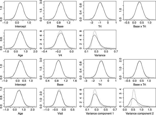
Figure 2: Marginal posterior distributions for parameters in model II (first two rows) and model IV (last two rows) of the epilepsy data estimated by MCMC (solid line) and Algorithm 3 using partially noncentered parametrization where tuning parameters are updated (dashed line).

is of the partially noncentered parametrization to the worst of the centered and noncentered parametrizations, since in general we do not know if centering or noncentering is better without running both algorithms. Partial noncentering, on the other hand, automatically chooses a near optimal parametrization. Updating of the tuning parameters helped to improve the fit produced by partial noncentering. Figure 2 shows the marginal posterior distributions for parameters in models II and IV estimated by MCMC (solid line) and Algorithm 3 using the partially noncentered parametrization where tuning parameters are updated (dashed line). The variational posterior densities of the fixed effects are very close to those obtained via MCMC. For the variance components, there is still some underestimation of the posterior variance.

6.3 Toenail Data

This data set was obtained from a multicenter study comparing two competing oral antifungal treatments for toenail infection (De Backer et al. (1998)), courtesy of Novoartis, Belgium. It contains information for 294 patients to be evaluated at seven visits. Not all patients attended all seven planned visits and there were 1908 measurements in total. The patients were randomized into two treatment groups, one group receiving 250 mg per day of terbinafine ($\mathrm{Trt}=1$) and the other group 200 mg per day of itraconazole ($\mathrm{Trt}=0$). Visits were planned at weeks 0, 4, 8, 12, 24, 36 and 48, but patients did not always arrive as scheduled and the exact time in months ($t$) that they did attend was recorded. The binary response variable (onycholysis) indicates the degree of separation of the nail plate from the nail bed (0 if none or mild, 1 if moderate or severe). We consider the following logistic random intercept model,

$$\operatorname{logit}(\mu_{ij})=\beta_{0}+\beta_{\mathrm{Trt}}\mathrm{Trt}_{i}+\beta_{t}t_{ij}+\beta_{\mathrm{Trt}\times t}\mathrm{Trt}_{i}\times t_{ij}+u_{i},$$

where $u_{i}\sim N(0,\sigma^{2})$ for $i=1,\ldots,294$, $1\leq j\leq 7$.

Table 3: Results for toenail data showing values used for initialization from penalized quasi-likelihood,posterior means and posterior standard deviations (values after $\pm$) from Algorithm 3 (different parametrizations)and MCMC, computation times (seconds) and variational lower bounds ($\mathcal{L}$)

	Penalized			Partially	Partially
	quasi-			noncentered:	noncentered:
	likelihood	Noncentered	Centered	$\bolds{W_{i}}$ fixed	$\bolds{W_{i}}$ updated	MCMC
$\beta_{0}$	$-0.75\pm 0.25$	$-1.41\pm 0.17$	$-1.44\pm 0.29$	$-1.44\pm 0.35$	$-1.44\pm 0.32$	$-1.65\pm 0.44$
$\beta_{\mathrm{Trt}}$	$-0.04\pm 0.35$	$-0.13\pm 0.25$	$-0.13\pm 0.41$	$-0.13\pm 0.49$	$-0.13\pm 0.45$	$-0.17\pm 0.60$
$\beta_{\mathrm{t}}$	$-0.30\pm 0.03$	$-0.38\pm 0.04$	$-0.38\pm 0.03$	$-0.38\pm 0.03$	$-0.38\pm 0.03$	$-0.40\pm 0.05$
$\beta_{\mathrm{Trt}\times\mathrm{Time}}$	$-0.10\pm 0.05$	$-0.13\pm 0.06$	$-0.13\pm 0.04$	$-0.13\pm 0.04$	$-0.13\pm 0.04$	$-0.14\pm 0.07$
$\sigma$	2.32	$3.52\pm 0.15$	$3.56\pm 0.15$	$3.55\pm 0.15$	$3.55\pm 0.15$	$4.10\pm 0.39$
$\mathcal{L}$	—	$-664.1$	$-663.1$	$-662.7$	$-662.9$	—
Time	2.8	37.9	27.9	26.0	24.1	1072

Table 3 shows the posterior means and standard deviations of the fits from MCMC and Algorithm 3 (using different parametrizations), initialization values from penalized quasi-likelihood and computation time in seconds taken by different methods. Again, the VB methods are faster than MCMC by an order of magnitude. In this example, centering produced a better fit than noncentering and partial noncentering produced a fit closer to that of the centered parametrization but improving it. Partial noncentering also took less time to converge and attained a lower bound higher than that of the centered and noncentered parametrizations. Again, we emphasize that it is not easy to know beforehand which of centering or noncentering will perform better, and a big advantage of partial noncentering is the way that it automatically chooses a good parametrization. In this example, updating the tuning parameters did not result in a better fit although the time to convergence is reduced.

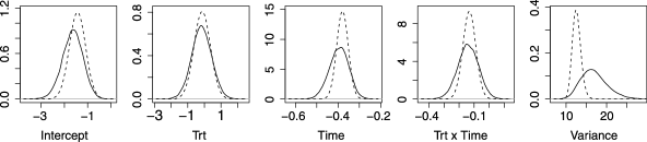
Figure 3: Marginal posterior distributions for parameters in toenail data estimated by MCMC (solid line) and Algorithm 3 using partially noncentered parametrization (tuning parameters not updated) (dashed line).

The marginal posterior distributions estimated byMCMC (solid line) and Algorithm 3 using the partially noncentered parametrization where tuning parameters were not updated (dashed line) are shown in Figure 3. Compared with the MCMC fit, there is still some underestimation of the variance of the fixed effects particularly for the parameters which could not be centered. Although the partially noncentered parametrization has improved the estimation of the random effects from the initial penalized quasi-likelihood fit, there is still some underestimation of the mean and variance of the random effects when compared to the MCMC fit.

6.4 Six Cities Data

In the previous two real data examples, centering performed better than noncentering and partial noncentering was able to improve on the centering results. While centering often performs better than noncentering, we use this example to show that partial noncentering will automatically tend toward noncentering when noncentering is preferred. We consider the six cities data in Fitzmaurice and Laird (1993), where the binary response variable $y_{ij}$ indicates the wheezing status (1 if wheezing, 0 if not wheezing) of the $i$th child at time-point $j$, $i=1,\ldots,537$, $j=1,2,3,4$. We use as covariate the age of the child at time-point $j$, centered at 9 years (Age), and consider the following random intercept and slope model:

$$\operatorname{logit}(\mu_{ij})=\beta_{0}+\beta_{\mathrm{Age}}\mathrm{Age}_{i}+u_{1i}+u_{2i}\mathrm{Age}_{i}$$

for $i=1,\ldots,537$, $j=1,\ldots,4$ and

$$\left[\matrix{u_{1i}\cr u_{2i}}\right]\sim N\left(0,\left[\matrix{\sigma_{11}^{2}&\sigma_{12}\cr\sigma_{21}&\sigma_{22}^{2}}\right]\right).$$

This model has been considered in Overstall and Forster (2010).

Table 4: Results for six cities data showing values used for initialization from penalized quasi-likelihood,posterior means and posterior standard deviations (values after $\pm$) from Algorithm 3 (different parametrizations)and MCMC, computation times (seconds) and variational lower bounds ($\mathcal{L}$)

	Penalized			Partially	Partially
	quasi-			noncentered:	noncentered:
	likelihood	Noncentered	Centered	$\bolds{W_{i}}$ fixed	$\bolds{W_{i}}$ updated	MCMC
$\beta_{0}$	$-3.12\pm 0.14$	$-3.05\pm 0.09$	$-3.05\pm 0.09$	$-3.05\pm 0.13$	$-3.05\pm 0.13$	$-3.29\pm 0.25$
$\beta_{\mathrm{Age}}$	$-0.24\pm 0.08$	$-0.22\pm 0.07$	$-0.21\pm 0.02$	$-0.22\pm 0.07$	$-0.22\pm 0.07$	$-0.25\pm 0.16$
$\sigma_{11}$	2.52	$2.16\pm 0.07$	$2.16\pm 0.07$	$2.16\pm 0.07$	$2.16\pm 0.07$	$2.48\pm 0.24$
$\sigma_{22}$	1.19	$0.55\pm 0.02$	$0.56\pm 0.02$	$0.55\pm 0.02$	$0.55\pm 0.02$	$0.61\pm 0.10$
$\mathcal{L}$	—	$-833.2$	$-834.1$	$-832.8$	$-832.6$	—
Time	3.8	114.7	125.8	110.6	120.6	1010

Table 4 shows the estimates of the posterior means and standard deviations of the fits from MCMC and Algorithm 3 using different parametrizations, the values from penalized quasi-likelihood used for initialization and the computation times in seconds taken by different methods. Noncentering performed better than centering in this case with a shorter time to convergence, higher lower bound and a better estimate of the posterior standard deviation of $\beta_{\mathrm{Age}}$. Partial noncentering further improved upon the results of noncentering with an improved estimate of the posterior standard deviation of $\beta_{0}$ and faster convergence. All the variational methods are again faster than MCMC by an order of magnitude.

6.5 Owl Data

In this example we illustrate the use of the variational lower bound, a by-product of Algorithm 3, for model selection. For MCMC, on the other hand, it is not straightforward in general to get a good estimate of the marginal likelihood based on the MCMC output. It is also not always obvious how to apply standard model selection criteria like AIC and BIC to hierarchical models like GLMMs.

Roulin and Bersier (2007) analyzed the begging behavior of nestling barn owls and looked at whether offspring beg for food at different intensities from the mother than father. They sampled $n=27$ nests and counted the number of calls made by all offspring in the absence of parents. Half of the nests were given extra prey, and from the other half prey were removed. Measurements took place on twonights, and food treatment was swapped the second night. The number of measurements at each nest ranged from 4 to 52 with a total of 599. We use as covariates sex of parent ($\mathrm{Sex}=1$ if male, 0 if female), the time at which a parent arrived with a prey ($t$), and food treatment ($\mathrm{Trt}=1$ if “satiated,” 0 if “deprived”). The number of nestlings per nest (broodsize, $E$) ranged from 1 to 7.

Table 5: Variational lower bounds for owl data models 1 to 11 and computation time in brackets

			Partially	Partially
			noncentered:	noncentered:
	Noncentered	Centered	$\bolds{W_{i}}$ fixed	$\bolds{W_{i}}$ updated
First stage
Model 1	$-$2544.6 (0.2)	$-$2543.7 (0.3)	$-$2543.6 (0.4)	$-$2543.7 (0.6)
Model 2	$-$2537.6 (0.2)	$-$2536.6 (0.3)	$-$2536.6 (0.4)	$-$2536.6 (0.5)
Model 3	$-$2540.2 (0.2)	$-$2539.2 (0.3)	$-$2539.2 (0.3)	$-$2539.2 (0.5)
Model 4	$-$2533.2 (0.2)	$-$2532.1 (0.3)	$-$2532.1 (0.3)	$-$2532.1 (0.4)
Second stage
Model 5	$-$2527.0 (0.2)	$-$2525.5 (0.2)	$-$2525.5 (0.2)	$-$2525.4 (0.3)
Model 6	$-$2628.3 (0.2)	$-$2627.2 (0.3)	$-$2627.1 (0.3)	$-$2627.1 (0.5)
Model 7	$-$2664.0 (0.2)	$-$2662.9 (0.2)	$-$2662.8 (0.3)	$-$2662.8 (0.4)
Third stage
Model 8	$-$2621.5 (0.2)	$-$2620.0 (0.2)	$-$2620.0 (0.2)	$-$2620.0 (0.3)
Model 9	$-$2660.4 (0.2)	$-$2658.8 (0.2)	$-$2658.8 (0.2)	$-$2658.8 (0.2)
Model 10	$-$2689.4 ($<$0.05)
Final stage
Model 11	$-$2448.7 (1.1)	$-$2445.7 (0.4)	$-$2445.8 (0.3)	$-$2445.6 (0.4)

Zuur et al. (2009) modeled the number of calls at nest $i$ for the $j$th observation as a Poisson distribution with mean $\mu_{ij}$ and used log transformed broodsize as an offset with nest as a random effect. The prime aim of their analysis was to find a sex effect and the largest model they considered was the following:

1. [10.]

2. $\log(\mu_{ij})=\log(E_{ij})+\beta_{0}+\beta_{\mathrm{Sex}}\mathrm{Sex}_{ij}+\beta_{\mathrm{Trt}}\mathrm{Trt}_{ij}+\beta_{t}t_{ij}+\beta_{\mathrm{Sex}\times\mathrm{Trt}}\mathrm{Sex}_{ij}\times\mathrm{Trt}_{ij}+\beta_{\mathrm{Sex}\times t}\mathrm{Sex}_{ij}\times t_{ij}+u_{i}$,

where $\log(E_{ij})$ is an offset and $u_{i}\sim N(0,\sigma^{2})$ for $i=1,\ldots,27$, $j=1,\ldots,n_{i}$. At the recommendation of Zuur et al. (2009), we center $t$ to reduce correlation of $t$ with the intercept. Henceforth, we assume $t_{ij}$ has been replaced by $t_{ij}-\operatorname{mean}(t)$. In the first stage, we consider models 1 to 4 and determine if the two interaction terms should be retained. Models 2 to 4 are as follows:

1. [10.]

2. $\log(\mu_{ij})=\log(E_{ij})+\beta_{0}+\beta_{\mathrm{Sex}}\mathrm{Sex}_{ij}+\beta_{\mathrm{Trt}}\mathrm{Trt}_{ij}+\beta_{t}t_{ij}+\beta_{\mathrm{Sex}\times\mathrm{Trt}}\mathrm{Sex}_{ij}\times\mathrm{Trt}_{ij}+u_{i}$,

3. $\log(\mu_{ij})=\log(E_{ij})+\beta_{0}+\beta_{\mathrm{Sex}}\mathrm{Sex}_{ij}+\beta_{\mathrm{Trt}}\mathrm{Trt}_{ij}+\beta_{t}t_{ij}+\beta_{\mathrm{Sex}\times t}\mathrm{Sex}_{ij}\times t_{ij}+u_{i}$,

4. $\log(\mu_{ij})=\log(E_{ij})+\beta_{0}+\beta_{\mathrm{Sex}}\mathrm{Sex}_{ij}+\beta_{\mathrm{Trt}}\mathrm{Trt}_{ij}+\beta_{t}t_{ij}+u_{i}$.

From Table 5, the preferred model (with the highest lower bound) is model 4 where both interaction terms have been dropped from model 1. Next, we consider models 5 to 7 where the main terms sex, food treatment and arrival time are each dropped in turn:

1. [10.]

2. $\log(\mu_{ij})=\log(E_{ij})+\beta_{0}+\beta_{\mathrm{Trt}}\mathrm{Trt}_{ij}+\beta_{t}t_{ij}+u_{i}$,

3. $\log(\mu_{ij})=\log(E_{ij})+\beta_{0}+\beta_{\mathrm{Trt}}\mathrm{Trt}_{ij}+\beta_{\mathrm{Sex}}\mathrm{Sex}_{ij}+u_{i}$,

4. $\log(\mu_{ij})=\log(E_{ij})+\beta_{0}+\beta_{t}t_{ij}+\beta_{\mathrm{Sex}}\mathrm{Sex}_{ij}+u_{i}$.

Table 5 indicates that model 5 is the preferred model where the term sex of the parent has been dropped from model 4. Now we consider dropping each of the terms food treatment and arrival time in turn or dropping the random effects $u_{i}$:

1. [10.]

2. $\log(\mu_{ij})=\log(E_{ij})+\beta_{0}+\beta_{\mathrm{Trt}}\mathrm{Trt}_{ij}+u_{i}$,

3. $\log(\mu_{ij})=\log(E_{ij})+\beta_{0}+\beta_{t}t_{ij}+u_{i}$,

4. $\log(\mu_{ij})=\log(E_{ij})+\beta_{0}+\beta_{\mathrm{Trt}}\mathrm{Trt}_{ij}+\beta_{t}t_{ij}$.

Table 5 indicates that none of the main terms food treatment and arrival time as well as random effects should be dropped from model 5. Finally, we consider adding a random slope for arrival time:

Table 6: Results for owl data (model 11) showing values used for initialization from penalized quasi-likelihood,posterior means and standard deviations (values after $\pm$) from Algorithm 3 (different parametrizations)and MCMC and computation times (seconds)

	Penalized			Partially	Partially
	quasi-			noncentered:	noncentered:
	likelihood	Noncentered	Centered	$\bolds{W_{i}}$ fixed	$\bolds{W_{i}}$ updated	MCMC
$\beta_{0}$	$0.60\pm 0.07$	$0.53\pm 0.02$	$0.51\pm 0.08$	$0.51\pm 0.08$	$0.51\pm 0.09$	$0.50\pm 0.10$
$\beta_{\mathrm{Trt}}$	$-0.55\pm 0.08$	$-0.57\pm 0.03$	$-0.57\pm 0.03$	$-0.57\pm 0.03$	$-0.57\pm 0.03$	$-0.57\pm 0.04$
$\beta_{t}$	$-0.13\pm 0.03$	$-0.15\pm 0.01$	$-0.16\pm 0.04$	$-0.16\pm 0.04$	$-0.16\pm 0.04$	$-0.16\pm 0.05$
$\sigma_{11}$	0.24	$0.44\pm 0.06$	$0.46\pm 0.06$	$0.45\pm 0.06$	$0.46\pm 0.06$	$0.47\pm 0.09$
$\sigma_{22}$	0.11	$0.22\pm 0.03$	$0.23\pm 0.03$	$0.22\pm 0.03$	$0.23\pm 0.03$	$0.23\pm 0.05$
Time	0.4	1.1	0.4	0.3	0.4	255

1. [11.]

2. $\log(\mu_{ij})=\log(E_{ij})+\beta_{0}+\beta_{\mathrm{Trt}}\mathrm{Trt}_{ij}+\beta_{t}t_{ij}+u_{1i}+u_{2i}t_{ij}$,

where

$$\left[\matrix{u_{1i}\cr u_{2i}}\right]\sim N\left(0,\left[\matrix{\sigma_{11}^{2}&\sigma_{12}\cr\sigma_{21}&\sigma_{22}^{2}}\right]\right).$$

From Table 5, the optimal model is model 11. This conclusion is similar to that of Zuur et al. (2009) and is the same regardless of which parametrization was used. It is thus sufficient to consider just the partially noncentered parametrization. The computation time taken by Algorithm 3 for each model fitting is very short and makes this a convenient way of carrying out model selection or for narrowing down the range of likely models. Further model comparisons can be performed using cross-validation or other approaches.

We present the estimated posterior means and standard deviations for the optimal model in Table 6. The marginal posterior distributions estimated by MCMC (solid line) and Algorithm 3 using partially noncentered parametrization where tuning parameters are updated (dashed line) are shown in Figure 4. In this case, centering produced a better fit than noncentering and partial

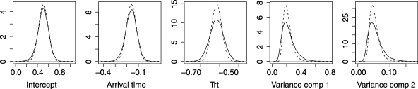
Figure 4: Marginal posterior distributions for parameters in model 11 (owl data) estimated by MCMC (solid line) and Algorithm 3 using partially noncentered parametrization where tuning parameters are updated (dashed line).

noncentering produced a fit that is close to that of centering. Updating the tuning parameters helped to improve the fit of the partially noncentered parametrization slightly and is closest to the MCMC fit. From the posterior density plots, there is good estimation of the posterior means by Algorithm 3 using partially noncentered parametrization with updated tuning parameters, but there is still some underestimation of the posterior variance.

7 Conclusion

In this paper we described a partially noncentered parametrization for GLMMs and compared the performance of different parametrizations using an algorithm called nonconjugate variational message passing developed recently in machine learning. Focusing on Poisson and logistic mixed models, we applied our methods to analysis of longitudinal data sets. For the logistic model, some parameter updates were not available in closed form and we used adaptive Gauss–Hermite quadrature to approximate the intractable integrals efficiently. Comparing the performance of Algorithm 3 under the partially noncentered parametrization with that of the centered and noncentered parametrizations, we observed that partial noncentering automatically tends toward the better of centering and noncentering so that it is not necessary to choose in advance between the centered and noncentered parametrizations. In many cases, the partially noncentered parametrization was able to improve upon the fit produced by the better of centering and noncentering to produce a fit that was closest to that of MCMC. In terms of computation time, the partially noncentered parametrization can also provide more rapid convergence when centering or noncentering is particularly slow. Very often, the lower bound attained by the partially noncentered parametrization is also higher than that of the centered and noncentered parametrizations, giving a tighter lower bound to the log marginal likelihood. To some degree, the partially noncentered parametrization also alleviates the issue of underestimation of the posterior variance, leading to some improvement in the estimation of the posterior variance, particularly in the fixed effects which could be centered. Algorithm 3 under the partially noncentered parametrization thus offers itself as a fast, deterministic alternative to MCMC methods for fitting GLMMs with improved estimation compared to the centered and noncentered parametrizations. We also demonstrate that the variational lower bound produced as part of the computation in Algorithm 3 can be useful in model selection.

Appendix A Evaluating the Variational Lower Bound

From (1.1), (3) and (18),

$$\mathcal{L} = \sum_{i=1}^{n}S_{y_{i}}+\sum_{i=1}^{n}S_{\tilde{\alpha}_{i}}+S_{\beta}+E_{q}\bigl{\{}\log p(D|\nu,S)\bigr{\}}$$

$${}-E_{q}\bigl{\{}\log q(\beta)\bigr{\}}-\sum_{i}^{n}E_{q}\bigl{\{}\log q(\tilde{\alpha}_{i})\bigr{\}}$$

$${}-E_{q}\bigl{\{}\log q(D)\bigr{\}}.$$

To evaluate the terms in the lower bound, we use the following two lemmas which we state without proof:

Lemma 1

Suppose $p_{1}(x)=N(\mu_{1},\Sigma_{1})$ and$p_{2}(x)=N(\mu_{2},\Sigma_{2})$ where $x$ is a $p$-dimensional vector, then $\int p_{2}(x)\log p_{1}(x)\,\mathrm{d}x=-\frac{p}{2}\log(2\pi)-\break{\frac{1}{2}\log}|\Sigma_{1}|-\frac{1}{2}(\mu_{2}-\mu_{1})^{T}\Sigma_{1}^{-1}(\mu_{2}-\mu_{1})-\frac{1}{2}\operatorname{tr}(\Sigma_{1}^{-1}\Sigma_{2})$.

Lemma 2

Suppose $p(D)=\mathit{IW}(\nu,S)$ where $D$ is a symmetric, positive definite $r\times r$ matrix, then ${\int p(D)\log}|D|\,\mathrm{d}D={\log}|S|-\sum_{l=1}^{r}\psi(\frac{\nu-l+1}{2})-r\log 2$ and $\int p(D)D^{-1}\,\mathrm{d}D=\nu S^{-1}$ where $\psi(\cdot)$ denotes the digamma function.

Using these two lemmas, we can compute most of the terms in the lower bound:

$$S_{\beta} = \int q(\beta)\log p(\beta|\Sigma_{\beta})\,\mathrm{d}\beta$$

$$= -\frac{p}{2}\log(2\pi)-{\frac{1}{2}\log}|\Sigma_{\beta}|$$

$${}-\frac{1}{2}{\mu_{\beta}^{q}}^{T}\Sigma_{\beta}^{-1}\mu_{\beta}^{q}-\frac{1}{2}\operatorname{tr}\bigl{(}\Sigma_{\beta}^{-1}\Sigma_{\beta}^{q}\bigr{)},$$

$$S_{\tilde{\alpha}_{i}} = \int q(\beta)q(D)q(\tilde{\alpha}_{i})\log p(\tilde{\alpha}_{i}|\beta,D)\,\mathrm{d}\beta\,\mathrm{d}D\,\mathrm{d}\tilde{\alpha}_{i}$$

$$= -\frac{r}{2}\log(2\pi)$$

$${}-\frac{1}{2}\Biggl{\{}\log\bigl{|}S^{q}\bigr{|}-\sum_{l=1}^{r}\psi\biggl{(}\frac{\nu^{q}-l+1}{2}\biggr{)}$$

$$\qquad\hskip 96.0pt{}-r\log 2\Biggr{\}}$$

$${}-\frac{\nu^{q}}{2}\bigl{[}\bigl{(}\mu_{\tilde{\alpha}_{i}}^{q}-\tilde{W}_{i}\mu_{\beta}^{q}\bigr{)}^{T}{S^{q}}^{-1}\bigl{(}\mu_{\tilde{\alpha}_{i}}^{q}-\tilde{W}_{i}\mu_{\beta}^{q}\bigr{)}$$

$$\hskip 53.1pt{}+\operatorname{tr}\bigl{\{}{S^{q}}^{-1}\bigl{(}\Sigma_{\tilde{\alpha}_{i}}^{q}+\tilde{W}_{i}\Sigma_{\beta}^{q}{\tilde{W}_{i}}^{T}\bigr{)}\bigr{\}}\bigr{]},$$

$$E_{q}\bigl{\{}\log p(D|\nu,S)\bigr{\}}$$

$$\quad=\int q(D)\log p(D|\nu,S)\,\mathrm{d}D$$

$$\quad=-\frac{\nu^{q}}{2}\operatorname{tr}\bigl{(}{S^{q}}^{-1}S\bigr{)}-\frac{r(r-1)}{4}\log(\pi)$$

$$\qquad{}-\sum_{l=1}^{r}\log\Gamma\biggl{(}\frac{\nu+1-l}{2}\biggr{)}+{\frac{\nu}{2}\log}|S|$$

$$\qquad{}-\frac{\nu+r+1}{2}\Biggl{\{}\log\bigl{|}S^{q}\bigr{|}-\sum_{l=1}^{r}\psi\biggl{(}\frac{\nu^{q}-l+1}{2}\biggr{)}$$

$$\qquad\hskip 155.5pt{}-r\log 2\Biggr{\}}$$

$$\qquad{}-\frac{\nu r}{2}\log 2,$$

$$E_{q}\bigl{\{}\log q(\beta)\bigr{\}}$$

$$\quad=\int q(\beta)\log q(\beta)\,\mathrm{d}\beta$$

$$\quad=-\frac{p}{2}\log(2\pi)-\frac{1}{2}\log\bigl{|}\Sigma_{\beta}^{q}\bigr{|}-\frac{p}{2},$$

$$E_{q}\bigl{\{}\log q(\tilde{\alpha}_{i})\bigr{\}}$$

$$\quad=\int q(\tilde{\alpha}_{i})\log q(\tilde{\alpha}_{i})\,\mathrm{d}\tilde{\alpha}_{i}$$

$$\quad=-\frac{r}{2}\log(2\pi)-\frac{1}{2}\log\bigl{|}\Sigma_{\tilde{\alpha}_{i}}^{q}\bigr{|}-\frac{r}{2},$$

$$E_{q}\bigl{\{}\log q(D)\bigr{\}}$$

$$\quad=\int q(D)\log q(D)\,\mathrm{d}D$$

$$\quad=-\frac{\nu^{q}r}{2}\log 2-\frac{r(r-1)}{4}\log\pi$$

$$\qquad{}-\sum_{l=1}^{r}\log\Gamma\biggl{(}\frac{\nu^{q}+1-l}{2}\biggr{)}+\frac{\nu^{q}}{2}\log\bigl{|}S^{q}\bigr{|}$$

$$\qquad{}-\frac{\nu^{q}+r+1}{2}\Biggl{\{}\log\bigl{|}S^{q}\bigr{|}-\sum_{l=1}^{r}\psi\biggl{(}\frac{\nu^{q}-l+1}{2}\biggr{)}$$

$$\qquad\hskip 160.0pt{}-r\log 2\Biggr{\}}$$

$$\qquad{}-\frac{\nu^{q}r}{2}.$$

The only term left to evaluate is

$$S_{y_{i}}=\int q(\beta)q(\tilde{\alpha}_{i})\log p(y_{i}|\beta,\tilde{\alpha}_{i})\,\mathrm{d}\beta\,\mathrm{d}\tilde{\alpha}_{i}.$$

For Poisson responses with the log link function[see (11)],

$$S_{y_{i}} = y_{i}^{T}\bigl{\{}\log(E_{i})+V_{i}\mu_{\beta}^{q}+X_{i}^{R}\mu_{\tilde{\alpha}_{i}}^{q}\bigr{\}}-E_{i}^{T}\kappa_{i}$$

$${}-1_{n_{i}}^{T}\log(y_{i}!),$$

where $\kappa_{i}=\exp\{V_{i}\mu_{\beta}^{q}+X_{i}^{R}\mu_{\tilde{\alpha}_{i}}^{q}+\frac{1}{2}\operatorname{diag}(V_{i}\Sigma_{\beta}^{q}{V_{i}}^{T}+X_{i}^{R}\Sigma_{\tilde{\alpha}_{i}}^{q}{X_{i}^{R}}^{T})\}$. For Bernoulli responses with the logit link function [see (3.1)],

$$S_{y_{i}} = y_{i}^{T}\bigl{(}V_{i}\mu_{\beta}^{q}+X_{i}^{R}\mu_{\tilde{\alpha}_{i}}^{q}\bigr{)}$$

$${}-\sum_{j=1}^{n_{i}}E_{q}\bigl{[}\log\bigl{\{}1+\exp\bigl{(}V_{ij}^{T}\beta+{X_{ij}^{R}}^{T}\tilde{\alpha}_{i}\bigr{)}\bigr{\}}\bigr{]},$$

where $E_{q}[\log\{1+\exp(V_{ij}^{T}\beta+{X_{ij}^{R}}^{T}\tilde{\alpha}_{i})\}]$ is evaluated using adaptive Gauss–Hermite quadrature (see Appendix B). The variational lower bound is thus given by

$$\mathcal{L} = \sum_{i=1}^{n}S_{y_{i}}+\frac{1}{2}\sum_{i=1}^{n}\log\bigl{|}\Sigma_{\tilde{\alpha}_{i}}^{q}\bigr{|}$$

$${}+\frac{1}{2}\log\bigl{|}\Sigma_{\beta}^{-1}\Sigma_{\beta}^{q}\bigr{|}-\frac{1}{2}\operatorname{tr}\bigl{(}\Sigma_{\beta}^{-1}\Sigma_{\beta}^{q}\bigr{)}$$

$${}-\frac{1}{2}{\mu_{\beta}^{q}}^{T}\Sigma_{\beta}^{-1}\mu_{\beta}^{q}-\frac{\nu^{q}}{2}\log\bigl{|}S^{q}\bigr{|}$$

$${}+{\frac{\nu}{2}\log}|S|-\sum_{l=1}^{r}\log\Gamma\biggl{(}\frac{\nu^{q}+1-l}{2}\biggr{)}$$

$${}+\sum_{l=1}^{r}\log\Gamma\biggl{(}\frac{\nu+1-l}{2}\biggr{)}$$

$${}+\frac{p+nr}{2}+\frac{nr}{2}\log 2.$$

Note that this expression is valid only after each of the parameter updates has been made in Algorithm 3.

Appendix B Gauss–Hermite Quadrature for Logistic Mixed Models

We want to evaluate $E_{q}\{b(V_{ij}^{T}\beta+{X_{ij}^{R}}^{T}\tilde{\alpha}_{i})\}$ where $b(x)=\log(1+\mathrm{e}^{x})$ for each $i=1,\ldots,n$ and $j=1,\ldots,\break n_{i}$. Let $\mu_{ij}=V_{ij}^{T}\mu_{\beta}^{q}+{X_{ij}^{R}}^{T}\mu_{\tilde{\alpha}_{i}}^{q}$ and $\sigma_{ij}^{2}=V_{ij}^{T}\Sigma_{\beta}^{q}V_{ij}+{X_{ij}^{R}}^{T}\Sigma_{\tilde{\alpha}_{i}}^{q}X_{ij}^{R}$. Following Ormerod and Wand (2012), we reduce $E_{q}\{b(V_{ij}^{T}\beta+{X_{ij}^{R}}^{T}\tilde{\alpha}_{i})\}$ to a univariate integral such that

$$E_{q}\bigl{\{}b\bigl{(}V_{ij}^{T}\beta+{X_{ij}^{R}}^{T}\tilde{\alpha}_{i}\bigr{)}\bigr{\}}$$

$$\quad=\int_{-\infty}^{\infty}b(\sigma_{ij}x+\mu_{ij})\phi(x;0,1)\,\mathrm{d}x,$$

where $\phi(x;\mu,\sigma)$ denotes the Gaussian density for a random variable $x$ with mean $\mu$ and standard deviation $\sigma$. Let $B^{(r)}(\mu,\sigma)=\int_{-\infty}^{\infty}b^{(r)}(\sigma x+\mu)\phi(x;0,1)\,\mathrm{d}x$ where $b^{(r)}(x)$ denotes the $r$th derivative of $b(\cdot)$ with respect to $x$. If $\mu$ and $\sigma$ are vectors, say,

$$\mu=\left[\matrix{1\cr 2\cr 3}\right]\quad\mbox{and}\quad\sigma=\left[\matrix{4\cr 5\cr 6}\right],$$

then

$$B^{(r)}(\mu,\sigma)=\left[\matrix{B^{(r)}(1,4)\vspace*{2pt}\cr B^{(r)}(2,5)\vspace*{2pt}\cr B^{(r)}(3,6)}\right].$$

For each cluster $i$, let $\mu_{i}=(\mu_{i1},\ldots,\mu_{in_{i}})^{T}=V_{i}\mu_{\beta}^{q}+X_{i}^{R}\mu_{\tilde{\alpha}_{i}}^{q}$ and

$$\sigma_{i} = (\sigma_{i1},\ldots,\sigma_{in_{i}})^{T}$$

$$= \sqrt{\operatorname{diag}\bigl{(}V_{i}\Sigma_{\beta}^{q}V_{i}^{T}+X_{i}^{R}\Sigma_{\tilde{\alpha}_{i}}^{q}{X_{i}^{R}}^{T}\bigr{)}}.$$

We evaluate $B^{(r)}(\mu_{ij},\sigma_{ij})$ using adaptive Gauss–Hermite quadrature (Liu and Pierce (1994)) for each $i=1,\ldots,n$, $j=1,\ldots,n_{i}$ and $r=0,1,2$. Ormerod and Wand (2012) have considered a similar approach. In Gauss–Hermite quadrature, integrals of the form $\int_{-\infty}^{\infty}f(x)\mathrm{e}^{-x^{2}}\,\mathrm{d}x$ are approximated by $\sum_{k=1}^{m}w_{k}f(x_{k})$, where $m$ is the number of quadrature points, the nodes $x_{i}$ are zeros of the $m$th order Hermite polynomial and $w_{i}$ are suitably corresponding weights. This approximation is exact for polynomials of degree $2m-1$ or less. For low-order quadrature to be effective, some transformation is usually required so that the integrand is sampled in a suitable range. Following the procedure recommended by Liu and Pierce (1994), we rewrite $B^{(r)}(\mu_{ij},\sigma_{ij})$ as

$$B^{(r)}(\mu_{ij},\sigma_{ij})$$

$$\quad=\int_{-\infty}^{\infty}\frac{b^{(r)}(\sigma_{ij}x+\mu_{ij})\phi(x;0,1)}{\phi(x;\hat{\mu}_{ij},\hat{\sigma}_{ij})}\phi(x;\hat{\mu}_{ij},\hat{\sigma}_{ij})\,\mathrm{d}x$$

$$\quad=\sqrt{2}\hat{\sigma}_{ij}\int_{-\infty}^{\infty}\bigl{[}\mathrm{e}^{x^{2}}b^{(r)}\bigl{(}\sigma_{ij}(\hat{\mu}_{ij}+\sqrt{2}\hat{\sigma}_{ij}x)+\mu_{ij}\bigr{)}$$

$$\qquad\hskip 97.7pt{}\cdot\phi(\hat{\mu}_{ij}+\sqrt{2}\hat{\sigma}_{ij}x;0,1)\bigr{]}$$

$$\qquad\hskip 48.7pt{}\cdot\mathrm{e}^{-x^{2}}\,\mathrm{d}x,$$

which can be approximated using Gauss–Hermite quadrature by

$$B^{(r)}(\mu_{ij},\sigma_{ij})$$

$$\quad\approx\sqrt{2}\hat{\sigma}_{ij}\sum_{k=1}^{m}w_{k}\mathrm{e}^{x_{k}^{2}}b^{(r)}\bigl{(}\sigma_{ij}(\hat{\mu}_{ij}+\sqrt{2}\hat{\sigma}_{ij}x_{k})+\mu_{ij}\bigr{)}$$

$$\hskip 66.6pt{}\cdot\phi(\hat{\mu}_{ij}+\sqrt{2}\hat{\sigma}_{ij}x_{k};0,1).$$

For the integrand to be sampled in an appropriate region, we take $\hat{\mu}_{ij}$ to be the mode of the integrand and $\hat{\sigma}_{ij}$ to be the standard deviation of the normal density approximating the integrand at the mode, so that

$$\hat{\mu}_{ij} = \mathop{\arg\max}_{x}\bigl{\{}b^{(r)}(\sigma_{ij}x+\mu_{ij})\phi(x;0,1)\bigr{\}},$$

$$\hat{\sigma}_{ij} = \biggl{[}-\frac{\mathrm{d}^{2}}{\mathrm{d}x^{2}}\log\bigl{\{}b^{(r)}(\sigma_{ij}x+\mu_{ij})$$

$$\hskip 75.0pt{}\cdot\phi(x;0,1)\bigr{\}}\bigg{|}_{x=\hat{\mu}_{ij}}\biggr{]}^{-{1/2}}$$

for $j=1,\ldots,n_{i}$ and $i=1,\ldots,n$. For computational efficiency, we evaluate $\hat{\mu}_{ij}$ and $\hat{\sigma}_{ij}$, $i=1,\ldots,n$, $j=1,\ldots,n_{i}$, for the case $r=1$ only once in each cycle of updates and use these values for $r=0,2$. No significant loss of accuracy was observed in doing this. We implement adaptive Gauss–Hermite quadrature in R using the R package fastGHQuad (Blocker (2011)). The quadrature nodes and weights can be obtained via the function gaussHermiteData() and the function aghQuad() approximates integrals using themethod of Liu and Pierce (1994). We used 10 quadrature points in all the examples.

References

- Attias (1999) {bincollection}[auto:STB—2013/03/04—13:35:07] \bauthor\bsnmAttias, \bfnmH.\binitsH. (\byear1999). \btitleInferring parameters and structure of latent variable models by variational Bayes. In \bbooktitleProceedings of the 15th Conference on Uncertainty in Artificial Intelligence \bpages21–30. \bpublisherMorgan Kaufmann, \blocationSan Francisco, CA. \bptokimsref \endbibitem
- Attias (2000) {bincollection}[auto:STB—2013/03/04—13:35:07] \bauthor\bsnmAttias, \bfnmH.\binitsH. (\byear2000). \btitleA variational Bayesian framework for graphical models. In \bbooktitleAdvances in Neural Information Processing Systems \bvolume12 \bpages209–215. \bpublisherMIT Press, \blocationCambridge, MA. \bptokimsref \endbibitem
- Bishop (2006) {bbook}[mr] \bauthor\bsnmBishop, \bfnmChristopher M.\binitsC. M. (\byear2006). \btitlePattern Recognition and Machine Learning. \bpublisherSpringer, \blocationNew York. \biddoi=10.1007/978-0-387-45528-0, mr=2247587 \bptokimsref \endbibitem
- Blocker (2011) {bmisc}[auto:STB—2013/03/04—13:35:07] \bauthor\bsnmBlocker, \bfnmA. W.\binitsA. W. (\byear2011). \bhowpublishedFast Rcpp implementation of Gauss–Hermite quadrature. R package “fastGHQuad” version 0.1-1. Available at http://cran.r-project.org/. \bptokimsref \endbibitem
- Braun and McAuliffe (2010) {barticle}[mr] \bauthor\bsnmBraun, \bfnmMichael\binitsM. and \bauthor\bsnmMcAuliffe, \bfnmJon\binitsJ. (\byear2010). \btitleVariational inference for large-scale models of discrete choice. \bjournalJ. Amer. Statist. Assoc. \bvolume105 \bpages324–335. \biddoi=10.1198/jasa.2009.tm08030, issn=0162-1459, mr=2757203 \bptokimsref \endbibitem
- Breslow and Clayton (1993) {barticle}[auto:STB—2013/03/04—13:35:07] \bauthor\bsnmBreslow, \bfnmN. E.\binitsN. E. and \bauthor\bsnmClayton, \bfnmD. G.\binitsD. G. (\byear1993). \btitleApproximate inference in generalized linear mixed models. \bjournalJ. Amer. Statist. Assoc. \bvolume88 \bpages9–25. \bptokimsref \endbibitem
- Brown and Zhou (2010) {barticle}[auto:STB—2013/03/04—13:35:07] \bauthor\bsnmBrown, \bfnmP.\binitsP. and \bauthor\bsnmZhou, \bfnmL.\binitsL. (\byear2010). \btitleMCMC for generalized linear mixed models with glmmBUGS. \bjournalThe R Journal \bvolume2 \bpages13–16. \bptokimsref \endbibitem
- Browne and Draper (2006) {barticle}[mr] \bauthor\bsnmBrowne, \bfnmWilliam J.\binitsW. J. and \bauthor\bsnmDraper, \bfnmDavid\binitsD. (\byear2006). \btitleA comparison of Bayesian and likelihood-based methods for fitting multilevel models. \bjournalBayesian Anal. \bvolume1 \bpages473–513 (electronic). \bidmr=2221283 \bptokimsref \endbibitem
- Cai and Dunson (2008) {bincollection}[mr] \bauthor\bsnmCai, \bfnmB.\binitsB. and \bauthor\bsnmDunson, \bfnmD. B.\binitsD. B. (\byear2008). \btitleBayesian variable selection in generalized linear mixed models. In \bbooktitleRandom Effect and Latent Variable Model Selection. \bseriesLecture Notes in Statistics \bvolume192 \bpages63–91. \bpublisherSpringer, \blocationNew York. \bptokimsref \endbibitem
- Christensen, Roberts and Sköld (2006) {barticle}[mr] \bauthor\bsnmChristensen, \bfnmOle F.\binitsO. F., \bauthor\bsnmRoberts, \bfnmGareth O.\binitsG. O. and \bauthor\bsnmSköld, \bfnmMartin\binitsM. (\byear2006). \btitleRobust Markov chain Monte Carlo methods for spatial generalized linear mixed models. \bjournalJ. Comput. Graph. Statist. \bvolume15 \bpages1–17. \biddoi=10.1198/106186006X100470, issn=1061-8600, mr=2269360 \bptokimsref \endbibitem
- Corduneanu and Bishop (2001) {bincollection}[auto:STB—2013/03/04—13:35:07] \bauthor\bsnmCorduneanu, \bfnmA.\binitsA. and \bauthor\bsnmBishop, \bfnmC. M.\binitsC. M. (\byear2001). \btitleVariational Bayesian model selection for mixture distributions. In \bbooktitleArtificial Intelligence and Statistics \bpages27–34. \bpublisherMorgan Kaufmann, \blocationSan Francisco, CA. \bptokimsref \endbibitem
- De Backer et al. (1998) {barticle}[auto:STB—2013/03/04—13:35:07] \bauthor\bsnmDe Backer, \bfnmM.\binitsM., \bauthor\bsnmDe Vroey, \bfnmC.\binitsC., \bauthor\bsnmLesaffre, \bfnmE.\binitsE., \bauthor\bsnmScheys, \bfnmI.\binitsI. and \bauthor\bsnmDe Keyser, \bfnmP.\binitsP. (\byear1998). \btitleTwelve weeks of continuous oral therapy for toenail onychomycosis caused by dermatophytes: A double-blind comparative trial of terbinafine 250 mg/day versus itraconazole 200 mg/day. \bjournalJournal of the American Academy of Dermatology \bvolume38 \bpages57–63. \bptokimsref \endbibitem
- Fitzmaurice and Laird (1993) {barticle}[auto:STB—2013/03/04—13:35:07] \bauthor\bsnmFitzmaurice, \bfnmG.\binitsG. and \bauthor\bsnmLaird, \bfnmN.\binitsN. (\byear1993). \btitleA likelihood-based method for analysing longitudinal binary responses. \bjournalBiometrika \bvolume80 \bpages141–151. \bptokimsref \endbibitem
- Fong, Rue and Wakefield (2010) {barticle}[auto:STB—2013/03/04—13:35:07] \bauthor\bsnmFong, \bfnmY.\binitsY., \bauthor\bsnmRue, \bfnmH.\binitsH. and \bauthor\bsnmWakefield, \bfnmJ.\binitsJ. (\byear2010). \btitleBayesian inference for generalised linear mixed models. \bjournalBiostatistics \bvolume11 \bpages397–412. \bptokimsref \endbibitem
- Gelfand, Sahu and Carlin (1995) {barticle}[mr] \bauthor\bsnmGelfand, \bfnmAlan E.\binitsA. E., \bauthor\bsnmSahu, \bfnmSujit K.\binitsS. K. and \bauthor\bsnmCarlin, \bfnmBradley P.\binitsB. P. (\byear1995). \btitleEfficient parameterisations for normal linear mixed models. \bjournalBiometrika \bvolume82 \bpages479–488. \biddoi=10.1093/biomet/82.3.479, issn=0006-3444, mr=1366275 \bptokimsref \endbibitem
- Gelfand, Sahu and Carlin (1996) {bincollection}[mr] \bauthor\bsnmGelfand, \bfnmA. E.\binitsA. E., \bauthor\bsnmSahu, \bfnmS. K.\binitsS. K. and \bauthor\bsnmCarlin, \bfnmB. P.\binitsB. P. (\byear1996). \btitleEfficient parametrizations for generalized linear mixed models. In \bbooktitleBayesian Statistics 5 (Alicante, 1994) \bpages165–180. \bpublisherOxford Univ. Press, \blocationNew York. \bidmr=1425405 \bptokimsref \endbibitem
- Gelman et al. (2004) {bbook}[mr] \bauthor\bsnmGelman, \bfnmAndrew\binitsA., \bauthor\bsnmCarlin, \bfnmJohn B.\binitsJ. B., \bauthor\bsnmStern, \bfnmHal S.\binitsH. S. and \bauthor\bsnmRubin, \bfnmDonald B.\binitsD. B. (\byear2004). \btitleBayesian Data Analysis, \bedition2nd ed. \bpublisherChapman & Hall/CRC, \blocationBoca Raton, FL. \bidmr=2027492 \bptnotecheck year\bptokimsref \endbibitem
- Ghahramani and Beal (2001) {bincollection}[auto:STB—2013/03/04—13:35:07] \bauthor\bsnmGhahramani, \bfnmZ.\binitsZ. and \bauthor\bsnmBeal, \bfnmM. J.\binitsM. J. (\byear2001). \btitlePropagation algorithms for variational Bayesian learning. In \bbooktitleAdvances in Neural Information Processing Systems \bvolume13 \bpages507–513. \bpublisherMIT Press, \blocationCambridge, MA. \bptokimsref \endbibitem
- Hoffman et al. (2012) {bmisc}[auto:STB—2013/03/04—13:35:07] \bauthor\bsnmHoffman, \bfnmM. D.\binitsM. D., \bauthor\bsnmBlei, \bfnmD. M.\binitsD. M., \bauthor\bsnmWang, \bfnmC.\binitsC. and \bauthor\bsnmPaisley, \bfnmJ.\binitsJ. (\byear2012). \bhowpublishedStochastic variational inference. Available at arXiv:\arxivurl1206.7051. \bptokimsref \endbibitem
- Jaakkola and Jordan (2000) {barticle}[auto:STB—2013/03/04—13:35:07] \bauthor\bsnmJaakkola, \bfnmT. S.\binitsT. S. and \bauthor\bsnmJordan, \bfnmM. I.\binitsM. I. (\byear2000). \btitleBayesian parameter estimation via variational methods. \bjournalStatist. Comput. \bvolume10 \bpages25–37. \bptokimsref \endbibitem
- Kass and Natarajan (2006) {barticle}[mr] \bauthor\bsnmKass, \bfnmRobert E.\binitsR. E. and \bauthor\bsnmNatarajan, \bfnmRanjini\binitsR. (\byear2006). \btitleA default conjugate prior for variance components in generalized linear mixed models (comment on article by Browne and Draper). \bjournalBayesian Anal. \bvolume1 \bpages535–542 (electronic). \bidmr=2221285 \bptokimsref \endbibitem
- Knowles and Minka (2011) {bmisc}[auto:STB—2013/03/04—13:35:07] \bauthor\bsnmKnowles, \bfnmD. A.\binitsD. A. and \bauthor\bsnmMinka, \bfnmT. P.\binitsT. P. (\byear2011). \bhowpublishedNon-conjugate variational message passing for multinomial and binary regression. In Advances in Neural Information Processing Systems 24 1701–1709. Available at http://books.nips.cc/ papers/files/nips24/NIPS2011_0962.pdf. \bptokimsref \endbibitem
- Liu and Pierce (1994) {barticle}[mr] \bauthor\bsnmLiu, \bfnmQing\binitsQ. and \bauthor\bsnmPierce, \bfnmDonald A.\binitsD. A. (\byear1994). \btitleA note on Gauss–Hermite quadrature. \bjournalBiometrika \bvolume81 \bpages624–629. \bidissn=0006-3444, mr=1311107 \bptokimsref \endbibitem
- Liu and Wu (1999) {barticle}[mr] \bauthor\bsnmLiu, \bfnmJun S.\binitsJ. S. and \bauthor\bsnmWu, \bfnmYing Nian\binitsY. N. (\byear1999). \btitleParameter expansion for data augmentation. \bjournalJ. Amer. Statist. Assoc. \bvolume94 \bpages1264–1274. \biddoi=10.2307/2669940, issn=0162-1459, mr=1731488 \bptokimsref \endbibitem
- Lunn et al. (2000) {barticle}[auto:STB—2013/03/04—13:35:07] \bauthor\bsnmLunn, \bfnmD. J.\binitsD. J., \bauthor\bsnmThomas, \bfnmA.\binitsA., \bauthor\bsnmBest, \bfnmN.\binitsN. and \bauthor\bsnmSpiegelhalter, \bfnmD.\binitsD. (\byear2000). \btitleWinBUGS—A Bayesian modelling framework: Concepts, structure, and extensibility. \bjournalStatist. Comput. \bvolume10 \bpages325–337. \bptokimsref \endbibitem
- Magnus and Neudecker (1988) {bbook}[mr] \bauthor\bsnmMagnus, \bfnmJan R.\binitsJ. R. and \bauthor\bsnmNeudecker, \bfnmHeinz\binitsH. (\byear1988). \btitleMatrix Differential Calculus with Applications in Statistics and Econometrics. \bpublisherWiley, \blocationChichester. \bidmr=0940471 \bptokimsref \endbibitem
- Meng and van Dyk (1997) {barticle}[mr] \bauthor\bsnmMeng, \bfnmXiao-Li\binitsX.-L. and \bauthor\bparticlevan \bsnmDyk, \bfnmDavid\binitsD. (\byear1997). \btitleThe EM algorithm—An old folk-song sung to a fast new tune (with discussion). \bjournalJ. R. Stat. Soc. Ser. B Stat. Methodol. \bvolume59 \bpages511–567. \biddoi=10.1111/1467-9868.00082, issn=0035-9246, mr=1452025 \bptokimsref \endbibitem
- Meng and van Dyk (1999) {barticle}[mr] \bauthor\bsnmMeng, \bfnmXiao-Li\binitsX.-L. and \bauthor\bparticlevan \bsnmDyk, \bfnmDavid A.\binitsD. A. (\byear1999). \btitleSeeking efficient data augmentation schemes via conditional and marginal augmentation. \bjournalBiometrika \bvolume86 \bpages301–320. \biddoi=10.1093/biomet/86.2.301, issn=0006-3444, mr=1705351 \bptokimsref \endbibitem
- O’Hagan and Forster (2004) {bbook}[auto:STB—2013/03/04—13:35:07] \bauthor\bsnmO’Hagan, \bfnmA.\binitsA. and \bauthor\bsnmForster, \bfnmJ.\binitsJ. (\byear2004). \btitleKendall’s Advanced Theory of Statistics V. 2B: Bayesian Inference, \bedition2nd ed. \bpublisherArnold, \blocationLondon. \bptokimsref \endbibitem
- Ormerod and Wand (2010) {barticle}[mr] \bauthor\bsnmOrmerod, \bfnmJ. T.\binitsJ. T. and \bauthor\bsnmWand, \bfnmM. P.\binitsM. P. (\byear2010). \btitleExplaining variational approximations. \bjournalAmer. Statist. \bvolume64 \bpages140–153. \biddoi=10.1198/tast.2010.09058, issn=0003-1305, mr=2757005 \bptokimsref \endbibitem
- Ormerod and Wand (2012) {barticle}[mr] \bauthor\bsnmOrmerod, \bfnmJ. T.\binitsJ. T. and \bauthor\bsnmWand, \bfnmM. P.\binitsM. P. (\byear2012). \btitleGaussian variational approximate inference for generalized linear mixed models. \bjournalJ. Comput. Graph. Statist. \bvolume21 \bpages2–17. \biddoi=10.1198/jcgs.2011.09118, issn=1061-8600, mr=2913353 \bptokimsref \endbibitem
- Overstall and Forster (2010) {barticle}[mr] \bauthor\bsnmOverstall, \bfnmAntony M.\binitsA. M. and \bauthor\bsnmForster, \bfnmJonathan J.\binitsJ. J. (\byear2010). \btitleDefault Bayesian model determination methods for generalised linear mixed models. \bjournalComput. Statist. Data Anal. \bvolume54 \bpages3269–3288. \biddoi=10.1016/j.csda.2010.03.008, issn=0167-9473, mr=2727751 \bptokimsref \endbibitem
- Papaspiliopoulos, Roberts and Sköld (2003) {bincollection}[mr] \bauthor\bsnmPapaspiliopoulos, \bfnmOmiros\binitsO., \bauthor\bsnmRoberts, \bfnmGareth O.\binitsG. O. and \bauthor\bsnmSköld, \bfnmMartin\binitsM. (\byear2003). \btitleNon-centered parameterizations for hierarchical models and data augmentation. In \bbooktitleBayesian Statistics 7 (Tenerife, 2002) \bpages307–326. \bpublisherOxford Univ. Press, \blocationNew York. \bidmr=2003180 \bptnotecheck related\bptokimsref \endbibitem
- Papaspiliopoulos, Roberts and Sköld (2007) {barticle}[mr] \bauthor\bsnmPapaspiliopoulos, \bfnmOmiros\binitsO., \bauthor\bsnmRoberts, \bfnmGareth O.\binitsG. O. and \bauthor\bsnmSköld, \bfnmMartin\binitsM. (\byear2007). \btitleA general framework for the parametrization of hierarchical models. \bjournalStatist. Sci. \bvolume22 \bpages59–73. \biddoi=10.1214/088342307000000014, issn=0883-4237, mr=2408661 \bptokimsref \endbibitem
- Qi and Jaakkola (2006) {bincollection}[auto:STB—2013/03/04—13:35:07] \bauthor\bsnmQi, \bfnmY.\binitsY. and \bauthor\bsnmJaakkola, \bfnmT. S.\binitsT. S. (\byear2006). \btitleParameter expanded variational Bayesian methods. In \bbooktitleAdvances in Neural Information Processing Systems \bvolume19 \bpages1097–1104. \bpublisherMIT Press, \blocationCambridge, MA. \bptokimsref \endbibitem
- Raudenbush, Yang and Yosef (2000) {barticle}[mr] \bauthor\bsnmRaudenbush, \bfnmStephen W.\binitsS. W., \bauthor\bsnmYang, \bfnmMeng-Li\binitsM.-L. and \bauthor\bsnmYosef, \bfnmMatheos\binitsM. (\byear2000). \btitleMaximum likelihood for generalized linear models with nested random effects via high-order, multivariate Laplace approximation. \bjournalJ. Comput. Graph. Statist. \bvolume9 \bpages141–157. \biddoi=10.2307/1390617, issn=1061-8600, mr=1826278 \bptokimsref \endbibitem
- Rijmen and Vomlel (2008) {barticle}[mr] \bauthor\bsnmRijmen, \bfnmFrank\binitsF. and \bauthor\bsnmVomlel, \bfnmJiří\binitsJ. (\byear2008). \btitleAssessing the performance of variational methods for mixed logistic regression models. \bjournalJ. Stat. Comput. Simul. \bvolume78 \bpages765–779. \biddoi=10.1080/00949650701282507, issn=0094-9655, mr=2528235 \bptokimsref \endbibitem
- Roos and Held (2011) {barticle}[mr] \bauthor\bsnmRoos, \bfnmMałgorzata\binitsM. and \bauthor\bsnmHeld, \bfnmLeonhard\binitsL. (\byear2011). \btitleSensitivity analysis in Bayesian generalized linear mixed models for binary data. \bjournalBayesian Anal. \bvolume6 \bpages259–278. \biddoi=10.1214/11-BA609, issn=1936-0975, mr=2806244 \bptokimsref \endbibitem