Oxygen and nitrogen abundances of H ii regions in six spiral galaxies

Abstract

Spectroscopic observations of 63 H ii regions in six spiral galaxies (NGC 628, NGC 783, NGC 2336, NGC 6217, NGC 7331, and NGC 7678) were carried out with the 6-meter telescope (BTA) of Russian Special Astrophysical Observatory with the Spectral Camera attached to the focal reducer SCORPIO in the multislit mode with a dispersion of 2.1Å/pixel and a spectral resolution of 10Å. These observations were used to estimate the oxygen and nitrogen abundances and the electron temperatures in H ii regions through the recent variant of the strong line method (NS calibration). The parameters of the radial distribution (the extrapolated central intercept value and the gradient) of the oxygen and nitrogen abundances in the disks of spiral galaxies NGC 628, NGC 783, NGC 2336, NGC 7331, and NGC 7678 have been determined. The abundances in the NGC 783, NGC 2336, NGC 6217, and NGC 7678 are measured for the first time. Galaxies from our sample follow well the general trend in the luminosity – central metallicity diagram for spiral and irregular galaxies.

1 Introduction

We have observed emission line spectra of 63 giant H ii regions in six spiral galaxies as a part of our study of star formation regions in spiral and irregular galaxies. Giant extragalactic H ii regions are the birth places of star clusters and can be used to study the current star formation and chemical abundances in galaxies. Giant H ii regions are ionised by clusters of young massive stars. Their sizes range from several tens to $\approx 500$ pc, so they are larger and brighter in comparison to Galactic H ii regions. Certain selection effects must be noted. Necessarily poorer spatial resolution contributes to a tendency to identify larger regions in more distant galaxies; at better resolution these regions break up into groups or chains of smaller clumps (Dinerstein, 1990).

One of the main interests in H ii regions is in the study of elemental abundances and their gradients in galaxies. A large number of regions have been observed for this purpose (Zaritsky et al., 1994; Roy et al., 1996; van Zee et al., 1998; Dutil & Roy, 1999; Kennicutt et al., 2003; Bresolin et al., 2005, 2009, among others). Radial distributions of oxygen and nitrogen abundances across the disks are mandatory in investigations of different aspects of formation and evolution of spiral galaxies. The measurement of the distribution of elemental abundances within galaxies is a tool for studying galaxy formation and evolution. There are several investigations of possible relationship between the abundances properties and global characteristics of galaxies such a Hubble type and luminosity (Pagel, 1991; Vila-Costas & Edmunds, 1992; Dutil & Roy, 1999; Garnett & Shields, 1987). The oxygen abundance in the interstellar gas is usually used as a tracer of metallicity in late type (spiral and irregular) galaxies at the current epoch. The study of abundance gradients in the disk of spiral galaxies has been started by Searle (1971), with the recognition of a radial abundance gradient in M33. Results of investigations of variations in the gas composition within galaxies combined with results on the evolution of stellar populations provide the development of chemical evolution models (Chiappini et al., 2003; Marcon-Uchida et al., 2010).

A study of abundances and their gradients is based on measurements of emission line spectra of individual H ii regions in nearby galaxies. To define the parameters of radial distribution of oxygen and nitrogen abundances (the extrapolated central intercept value and the gradient), the abundance measurements for a sufficiently large number of H ii regions evenly distributed across the galaxy disk are necessary. Measurements of this kind are available for the limited number ($\sim$50) of nearby galaxies (see compilations in Garnett, 2002; Pilyugin et al., 2004; Moustakas et al., 2010).

Table 1: The galaxy sample.

Galaxy	Type	$B_{t}$	RAa	DECa	Inclination	P.A.	$v^{b}$	$R_{25}^{c}$	$R_{25}^{c}$	$d$	$M_{B}$
		(mag)	(J2000.0)	(J2000.0)	(degree)	(degree)	(km/s)	(arcmin)	(kpc)	(Mpc)	(mag)
1	2	3	4	5	6	7	8	9	10	11	12
NGC 628	Sc	9.70	01 36 41.81	+15 47 00.3	7	25	659	5.23	10.96	7.2	-20.72
NGC 783	Sc	13.18	02 01 06.59	+31 52 56.2	43	57	5192	0.71	14.56	70.5	-22.01
NGC 2336	SB(R)bc	11.19	07 27 03.98	+80 10 41.1	55	175	2202	2.51	23.51	32.2	-22.14
NGC 6217	SB(R)bc	11.89	16 32 39.28	+78 11 53.6	33	162	1368	1.15	6.89	20.6	-20.45
NGC 7331	Sbc	10.20	22 37 04.16	+34 24 56.0	75	169	818	4.89	20.06	14.1	-21.68
NGC 7678	SBc	12.50	23 28 27.87	+22 25 14.0	44	21	3488	1.04	14.46	47.8	-21.55

^a Coordinates of the galaxy center. Units of right ascension are hours, minutes, and seconds, and units of declination are degrees, arcminutes, and arcseconds. ^b Heliocentric radial velocity. ^c Isophotal radius (25 mag/arcsec² in the $B$-band) corrected for Galactic extinction and absorption due to the inclination of a galaxy.

Table 2: Journal of observations.

Object (Pos.a)	Date	Exposures	Seeing	Airmass
		(s)	(arcsec)
NGC 628 (1)	2008.02.07	$900\times 2$	1.9	2.03
NGC 783 (1)	2006.10.19	$900\times 3$	3.0	1.28
NGC 783 (2)	2007.09.07	$900\times 4$	1.6	1.02
NGC 783 (3)	2008.02.09	$900\times 6$	1.9	1.29
NGC 2336 (1)	2006.10.19	$900\times 4$	2.0	1.39
NGC 2336 (2)	2008.02.08	$900\times 8$	1.4	1.31
NGC 2336 (3)	2006.10.19	$300+900$	2.0	1.32
NGC 2336 (4)	2008.02.09	$900\times 6$	1.2	1.33
NGC 6217 (1)	2006.08.23	$900\times 4$	1.8	1.47
NGC 7331 (1)	2006.08.23	$900\times 4$	2.1	1.17
NGC 7678 (1)	2006.08.22	$900\times 3$	1.4	1.15
NGC 7678 (2)	2006.10.19	$900\times 2$	1.6	1.08
NGC 7678 (3)	2006.10.19	$900\times 3$	1.6	1.08

^a Slit position

Here we report spectra of 63 H ii regions in a sample of six spiral galaxies: NGC 628, NGC 783, NGC 2336, NGC 6217, NGC 7331, and NGC 7678. A first motivation of the spectral observations is the determination of the oxygen and nitrogen abundances and electron temperatures in individual H ii regions using the recent NS- and ON calibration (Pilyugin et al., 2010; Pilyugin & Mattsson, 2011). The abundances will be used in the computation of the grid of evolutionary models of star clusters embedded in studied H ii regions. The second motivation is the determination of the optical extinction by dust to the gas, from the measured Balmer decrement in the studied H ii regions.

In this paper we describe observations and data reduction, the derivation of elemental abundances, electron temperatures and optical extinction for individual H ii regions and the examination their radial gradients across the disks. Results of these examinations provide information about the chemical abundance of interstellar medium from which embedded stars formed, as well as the dust extinction estimations in the surrounding gas.

The paper is organized as follows. The observations and data reduction are described in Section 2. The oxygen and nitrogen abundances and the electron temperatures for individual H ii regions as well the parameters of the radial distributions (the extrapolated central intercept value and the gradient) of the oxygen and nitrogen abundances and electron temperature in galaxies are discussed in Section 3. Section 4 gives a brief summary.

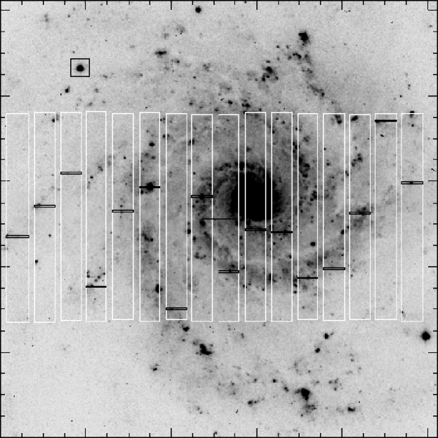
Figure 1: Disposition of 16 slits (black small horizontal rectangles) for NGC 628. North is upward and east is to the left (P.A.${}_{slits}=90\degr$). The size of the image is $6.1\times 6.1$ arcmin². The black square shows a guide star for the exposures.

Throughout the paper, we will be using the following notations for the line fluxes,

$$R_{2}=[{\rm O}\,\textsc{ii}]\lambda 3727+\lambda 3729=I_{\rm[OII]\lambda 3727+\lambda 3729}/I_{{\rm H}\beta},$$ (1)

$$N_{2}=[{\rm N}\,\textsc{ii}]\lambda 6548+\lambda 6584=I_{\rm[NII]\lambda 6548+\lambda 6584}/I_{{\rm H}\beta},$$ (2)

$$S_{2}=[{\rm S}\,\textsc{ii}]\lambda 6717+\lambda 6731=I_{\rm[SII]\lambda 6717+\lambda 6731}/I_{{\rm H}\beta},$$ (3)

$$R_{3}=[{\rm O}\,\textsc{iii}]\lambda 4959+\lambda 5007=I_{{\rm[OIII]}\lambda 4959+\lambda 5007}/I_{{\rm H}\beta}.$$ (4)

The electron temperatures $t$ are given in units of 10⁴K.

2 OBSERVATIONS AND REDUCTION

Table 3: Offsets, galactocentric distances, radial velocities of H ii regions.

H ii	Pos.a	Ref.b	N–Sc	E–Wc	$r^{d}$	$v^{e}$
region			(arcsec)	(arcsec)	(kpc)	(km/s)
NGC 628
1	1	94, 54	+12.5	+129.0	4.55	620
2	1	92	-12.0	+87.7	3.11	665
3	1	77, 58	-64.3	+36.5	2.58	611
4	1	75	-65.4	+45.0	2.77	638
5	1	73, 11	-28.8	+25.3	1.34	654
6	1	25, 6	+0.2	-43.0	1.51	655
7	1	62, 81	-91.8	-68.1	4.01	628
8	1	58	-72.0	-132.6	5.31	614
9	1	35	+19.7	-153.1	5.42	716
10	1	38, (5)	-6.4	-177.9	6.25	711
NGC 783
1	1	—	-24.3	+16.0	10.60	5181
2	1	—	-27.5	+23.7	12.83	5202
3	1	—	-4.8	-19.7	8.33	5192
4	1	—	+19.5	-29.1	11.96	5235
5	2	—	-19.5	+22.1	10.17	5270
6	2	—	-20.0	+25.6	11.15	5103
7	2	—	+21.6	-28.3	12.20	5153
8	3	—	+5.1	-22.9	8.42	5233
NGC 2336
1a	1	—	-113.8	+33.5	20.79	2011
1b	2	—	-113.8	+33.5	20.79	2048
2	1	28	-89.0	-40.0	16.89	2006
3	1	27a	-71.8	+0.2	11.30	2040
4a	1	26	-47.8	-10.5	7.79	2009
4b	4	26	-47.8	-10.5	7.79	2052
5	1	22	-27.5	-9.8	4.86	2028
6	1	17	+17.5	+85.4	23.02	2264
7a	1	5	+95.9	+13.6	15.19	2432
7b	2	5	+95.9	+13.6	15.19	2410
8	2	27d	-82.5	-9.5	12.99	2013
9	2	—	-62.6	+8.1	10.27	1917
10a	2	19	+3.4	+43.8	11.82	2141
10b	4	19	+3.4	+43.8	11.82	2198
11	2	16	+18.2	+38.7	10.59	2349
12	2	10	+52.3	+0.2	8.22	2512
13	2	8	+68.1	-34.5	14.84	2485
14a	2	2	+142.0	-11.5	22.83	2573
14b	4	2	+142.0	-11.5	22.83	2545
15a	3	30	-109.0	-32.1	18.49	1940
15b	4	30	-109.0	-32.1	18.49	1935
16a	3	27b	-77.3	-3.6	12.11	2014
16b	4	27b	-77.3	-3.6	12.11	2018
17a	3	21	-26.1	+48.3	14.05	2167
17b	4	21	-26.1	+48.3	14.05	2061
18	4	29	-94.5	-37.3	17.18	2233
19	4	27e	-83.9	-4.3	13.13	2064
20	4	—	-31.6	+48.6	14.49	2160
21	4	—	-19.3	+47.6	13.50	1982
22	4	—	+27.2	-62.7	17.88	2364
23	4	15	+24.4	-61.7	17.47	2263
24	4	9	+62.6	+48.3	15.61	2375
25	4	—	+67.7	+44.5	15.32	2443
26	4	—	+77.7	-5.3	12.43	2575
27	4	7	+80.8	-4.6	12.88	2422
28	4	4	+111.7	-31.1	20.17	2335
NGC 6217
1	1	—	+29.8	+13.9	3.30	1443
2	1	—	+42.2	+13.0	4.41	1485
3	1	—	-14.6	+23.2	3.24	1348

Table 3: Continued

H ii	Pos.a	Ref.b	N–Sc	E–Wc	$r^{d}$	$v^{e}$
region			(arcsec)	(arcsec)	(kpc)	(km/s)
NGC 7331
1	1	—	+123.2	+40.4	9.78	537
2	1	—	+76.8	+18.0	5.45	512
3	1	—	+27.4	+16.2	3.48	667
4	1	1	-50.2	+23.1	9.06	865
NGC 7678
1	1	—	-54.2	+12.6	13.02	3422
2	1	—	-31.8	-7.1	8.57	3431
3	1	—	-23.3	-14.8	8.10	3525
4	1	—	-14.5	-21.0	8.11	3553
5	1	—	+3.7	-26.6	8.15	3455
6	2	—	-26.5	+14.2	7.02	3412
7	2	—	-10.5	+31.6	9.63	3415
8a	2	—	-15.8	+27.3	8.56	3426
8b	3	—	-15.8	+27.3	8.56	3432
9	3	—	-46.5	-5.2	11.87	3384
10	3	—	-23.0	+6.2	5.56	3398

^a Slit position. ^b H ii region number from Belley & Roy (1992) (first number), from Rosales-Ortega et al. (2011) (second number), and from van Zee et al. (1998) (second number in brackets) for NGC 628, from Gusev & Park (2003) for NGC 2336, and from Bresolin et al. (1999) for NGC 7331. ^c Offsets from the galactic centre (see Table 1), positive to the north and west. ^d Deprojected galactocentric distance.

^e Radial velocity of H ii region (km s^-1).

We selected galaxies with known $UBVRI$ photometry of H ii regions, obtained by our team in the previous works: NGC 628 (Bruevich et al., 2007), NGC 783 (Gusev, 2006a, b), NGC 2336 (Gusev & Park, 2003), NGC 6217 (Artamonov et al., 1999), NGC 7331 (unpublished), NGC 7678 (Artamonov et al., 1997). The galaxy sample is presented in Table 1. The columns show parameters from the leda data base (Paturel at al., 2003): morphological type and apparent magnitude of the galaxy in columns (2) and (3), coordinates (epoch 2000) in columns (4) and (5), the inclination and position angles in columns (6) and (7), radial velocity in column (8), the isophotal radius in arcmin and kpc in columns (9) and (10), distance in the column (11), the absolute blue magnitude $M_{B}$ in column (12).

2.1 Observations

The observations were carried out at the 6 m telescope of Special Astrophysical Obsevatory (SAO) of the Russian Academy of Sciences with Spectral Camera attached at the focal reducer SCORPIO (Afanasiev & Moiseev, 2005) ($f/4\to f/2.6$) in the multislit mode; the field was about 6 arcmin and the pixel size was 0.178 arcsec on a EEV 42-40 ($2048\times 2048$ pixels) CCD detector. The data for six galaxies were acquired during observing runs in 2006–2008 (see the journal of observations in Table 2).

The SCORPIO multislit unit is an arrangement that consists of 16 metal strips with slits located in the focal plane and moved in a $2.9\times 5.9$ arcmin² field (Fig. 1). The size of slits is $1.5\times 18$ arcsec², the distance between centres of neighbouring slits is 22 arcsec.

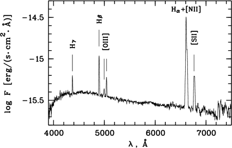
Figure 2: The observed spectrum ”b” of the H ii region 17 in NGC 2336.

We used the grism VPHG550G with a dispersion of 2.1Å/pixel and a spectral resolution of 10Å, which provided spectral coverage from [O ii]$\lambda$3727+$\lambda$3729 oxygen emission lines to [S ii]$\lambda$6717+$\lambda$6731 sulphur emission lines. The example of spectrum is presented in Fig. 2.

We selected target H ii regions using $B$ band and H$\alpha$ CCD images of galaxies, which were obtained with the 1 m and 1.5 m telescopes of the Mt. Maidanak Observatory (Institute of Astronomy, Uzbek Academy of Sciences) in Uzbekistan and with the 1.8 m telescope of the Bohyunsan Optical Astronomy Observatory (Korea Astronomy and Space Science Institute) in Korea.

As mentioned above, the broadband $UBVRI$ photometry of selected H ii regions, derived previously by us and our colleagues as a part of our study of star formation processes in spiral and irregular galaxies, provided the source of targets for the multi-slit observations. We selected objects widely distributed across the face of the galaxies, enabling the study of the chemical abundance gradients. The H ii regions were selected for spectroscopy based on their brightness and size, with typical angular diameters from 2 up to 5 arcsec.

The total exposure time of the set consists of several time intervals. After the every time interval, positions of slits were displaced along the X axes with a step of 20 pixels. X axes runs along the slit and Y axes runs perpendicularly to the slit (see Fig. 1). This technique allows us to obtain spectra of several neighbouring H ii regions using the same slit. Therefore, the exposure time for individual H ii regions was smaller than the total exposure time of the set indicated in the Table 2.

The observing procedure consisted of obtaining bias, flat and wavelength calibration images at the beginning and the end of the each set. Several spectrophotometric standards were observed during the each night at different air mass.

Table 4: The reddening-corrected fluxes of main emission lines of H ii regions.

H ii	[O ii]a	[O iii]a	[N ii]a	[S ii]a	$F$(H$\beta$)b	$c$(H$\beta$)
region	3727+3729	5007	6584	6717+6731	4861
NGC 628
1	—	—	0.73$\pm$0.41	0.42$\pm$0.24	7.48$\pm$1.17	0.74$\pm$0.31
2	—	—	1.06$\pm$0.42	1.16$\pm$0.45	8.04$\pm$0.85	0.58$\pm$0.24
3	—	—	0.61$\pm$0.26	0.35$\pm$0.14	27.40$\pm$3.07	0.33$\pm$0.21
4	—	0.31$\pm$0.13	0.46$\pm$0.35	0.54$\pm$0.30	5.21$\pm$0.79	0.37$\pm$0.31
5	—	—	0.70$\pm$0.35	0.78$\pm$0.35	9.61$\pm$1.08	0.30$\pm$0.25
6	—	—	—	—	2.12$\pm$0.80	0.85$\pm$0.96
7	5.64$\pm$2.01	0.49$\pm$0.07	0.79$\pm$0.22	0.47$\pm$0.12	33.32$\pm$1.82	0.00$\pm$0.13
8	4.06$\pm$1.74	0.66$\pm$0.07	0.77$\pm$0.18	0.51$\pm$0.10	38.15$\pm$2.05	0.12$\pm$0.12
9	—	1.62$\pm$0.18	0.59$\pm$0.16	0.32$\pm$0.08	22.62$\pm$1.41	0.87$\pm$0.13
10	—	0.36$\pm$0.10	0.74$\pm$0.29	0.77$\pm$0.30	30.51$\pm$3.80	0.03$\pm$0.22
NGC 783
1	—	1.47$\pm$0.20	1.06$\pm$0.27	0.72$\pm$0.20	5.81$\pm$0.38	0.28$\pm$0.15
2	—	0.73$\pm$0.30	—	—	1.38$\pm$0.36	0.08$\pm$0.55
3	1.80$\pm$0.60	0.23$\pm$0.04	1.33$\pm$0.20	0.89$\pm$0.13	22.15$\pm$6.51	0.51$\pm$0.09
4	—	0.68$\pm$0.13	1.46$\pm$0.46	1.19$\pm$0.39	3.34$\pm$0.29	0.90$\pm$0.20
5	2.34$\pm$0.68	0.23$\pm$0.04	0.54$\pm$0.14	0.86$\pm$0.15	7.78$\pm$0.31	0.61$\pm$0.10
6	2.45$\pm$0.53	0.44$\pm$0.05	1.50$\pm$0.21	1.16$\pm$0.17	11.69$\pm$0.42	0.44$\pm$0.09
7	—	1.25$\pm$0.46	3.11$\pm$1.87	2.30$\pm$1.46	2.55$\pm$0.46	0.76$\pm$0.45
8	2.35$\pm$0.54	0.32$\pm$0.06	1.16$\pm$0.19	0.64$\pm$0.12	25.97$\pm$1.00	0.73$\pm$0.09
NGC 2336
1a	—	0.61$\pm$0.23	1.15$\pm$0.59	1.05$\pm$0.53	2.04$\pm$0.35	0.46$\pm$0.33
1b	4.16$\pm$1.07	1.01$\pm$0.11	0.89$\pm$0.18	1.37$\pm$0.24	6.80$\pm$0.33	0.15$\pm$0.11
2	2.26$\pm$0.66	0.58$\pm$0.05	0.81$\pm$0.12	0.51$\pm$0.07	22.07$\pm$0.77	0.45$\pm$0.08
3	—	0.27$\pm$0.07	0.80$\pm$0.23	0.44$\pm$0.14	16.36$\pm$1.18	0.69$\pm$0.16
4a	—	—	0.66$\pm$0.16	0.47$\pm$0.10	7.83$\pm$0.40	0.71$\pm$0.12
4b	—	—	0.82$\pm$0.22	0.57$\pm$0.15	22.58$\pm$1.29	0.34$\pm$0.14
5	—	—	0.91$\pm$0.56	—	2.70$\pm$0.31	0.34$\pm$0.32
6	—	1.42$\pm$0.06	0.48$\pm$0.08	0.62$\pm$0.07	19.92$\pm$0.53	1.12$\pm$0.06
7a	—	0.48$\pm$0.09	0.85$\pm$0.23	0.66$\pm$0.19	5.37$\pm$0.38	0.46$\pm$0.15
7b	—	0.27$\pm$0.02	0.88$\pm$0.11	0.66$\pm$0.08	35.97$\pm$0.98	0.45$\pm$0.06
8	2.21$\pm$0.48	0.14$\pm$0.02	0.71$\pm$0.11	0.66$\pm$0.08	28.12$\pm$0.70	0.32$\pm$0.07
9	—	0.05$\pm$0.01	0.77$\pm$0.13	0.60$\pm$0.09	20.06$\pm$0.56	0.11$\pm$0.08
10a	—	0.16$\pm$0.03	1.07$\pm$0.17	0.80$\pm$0.13	18.14$\pm$0.63	0.46$\pm$0.09
10b	—	0.17$\pm$0.02	1.01$\pm$0.13	0.70$\pm$0.08	33.81$\pm$0.96	0.64$\pm$0.07
11	—	0.47$\pm$0.08	1.17$\pm$0.27	1.14$\pm$0.26	8.42$\pm$0.55	0.90$\pm$0.14
12	—	—	0.85$\pm$0.36	0.79$\pm$0.34	4.94$\pm$0.62	0.93$\pm$0.26
13	—	0.35$\pm$0.04	1.04$\pm$0.15	0.60$\pm$0.09	11.16$\pm$0.38	1.23$\pm$0.08
14a	—	1.15$\pm$0.10	0.91$\pm$0.16	0.98$\pm$0.16	18.31$\pm$0.82	0.72$\pm$0.10
14b	3.36$\pm$0.76	1.18$\pm$0.07	0.79$\pm$0.11	0.87$\pm$0.10	20.25$\pm$0.66	0.70$\pm$0.07
15a	—	1.68$\pm$0.54	0.65$\pm$0.51	—	2.47$\pm$0.44	0.21$\pm$0.40
15b	6.36$\pm$2.07	0.89$\pm$0.11	0.66$\pm$0.18	0.78$\pm$0.20	9.32$\pm$0.47	0.07$\pm$0.13
16a	2.07$\pm$0.92	0.32$\pm$0.08	0.73$\pm$0.20	0.79$\pm$0.20	9.31$\pm$0.65	0.66$\pm$0.15
16b	2.63$\pm$0.61	0.21$\pm$0.03	0.73$\pm$0.12	0.68$\pm$0.09	26.12$\pm$0.75	0.56$\pm$0.07
17a	—	0.25$\pm$0.06	0.92$\pm$0.25	0.73$\pm$0.20	15.98$\pm$1.32	0.38$\pm$0.16
17b	—	0.32$\pm$0.02	1.22$\pm$0.11	0.65$\pm$0.05	99.43$\pm$1.82	0.62$\pm$0.05
18	—	—	0.75$\pm$0.47	0.89$\pm$0.56	3.63$\pm$0.66	1.32$\pm$0.38
19	7.54$\pm$2.31	0.23$\pm$0.07	0.72$\pm$0.20	0.82$\pm$0.20	13.78$\pm$0.88	0.71$\pm$0.14
20	—	0.24$\pm$0.08	1.11$\pm$0.25	0.89$\pm$0.21	8.53$\pm$0.57	1.06$\pm$0.13
21	—	0.30$\pm$0.05	1.73$\pm$0.31	0.94$\pm$0.20	8.93$\pm$0.43	0.35$\pm$0.12
22	1.78$\pm$0.29	0.53$\pm$0.02	0.81$\pm$0.08	0.60$\pm$0.05	22.86$\pm$0.44	0.49$\pm$0.05
23	1.88$\pm$0.25	0.68$\pm$0.02	0.85$\pm$0.08	0.60$\pm$0.04	42.42$\pm$0.74	0.09$\pm$0.04
24	—	0.76$\pm$0.20	1.33$\pm$0.52	1.24$\pm$0.52	3.62$\pm$0.42	0.84$\pm$0.25
25	—	0.82$\pm$0.16	0.87$\pm$0.25	0.71$\pm$0.22	5.12$\pm$0.41	0.86$\pm$0.17
26	—	0.47$\pm$0.22	1.34$\pm$0.64	1.13$\pm$0.55	5.96$\pm$0.93	0.92$\pm$0.32
27	—	0.72$\pm$0.22	1.39$\pm$0.56	1.21$\pm$0.54	4.56$\pm$0.44	0.50$\pm$0.25
28	2.37$\pm$0.40	0.70$\pm$0.03	0.89$\pm$0.09	0.69$\pm$0.08	38.60$\pm$0.81	0.08$\pm$0.05
NGC 6217
1	1.87$\pm$0.81	0.25$\pm$0.05	0.85$\pm$0.16	0.52$\pm$0.10	21.24$\pm$0.86	0.10$\pm$0.10
2	—	—	1.09$\pm$0.52	0.89$\pm$0.42	7.37$\pm$1.14	0.76$\pm$0.31

^a $I$($\lambda$)/$I$(H$\beta$) ratio. ^b The fluxes are in units of $10^{-16}$ erg  s^-1 cm^-2.

Table 4: Continued

H ii	[O ii]a	[O iii]a	[N ii]a	[S ii]a	$F$(H$\beta$)b	$c$(H$\beta$)
region	3727+3729	5007	6584	6717+6731	4861
NGC 6217
3	—	0.98$\pm$0.31	1.08$\pm$0.43	0.71$\pm$0.29	7.70$\pm$1.03	0.80$\pm$0.25
NGC 7331
1	—	1.05$\pm$0.22	1.20$\pm$0.57	0.91$\pm$0.44	3.16$\pm$0.36	0.09$\pm$0.28
2	—	—	2.65$\pm$2.33	0.91$\pm$0.90	1.13$\pm$0.31	1.53$\pm$0.68
3	—	0.14$\pm$0.06	0.44$\pm$0.16	0.26$\pm$0.09	9.27$\pm$0.79	1.24$\pm$0.17
4	2.32$\pm$1.15	0.41$\pm$0.04	0.99$\pm$0.14	0.82$\pm$0.10	26.64$\pm$0.88	0.50$\pm$0.08
NGC 7678
1	—	1.17$\pm$0.58	0.82$\pm$0.68	0.88$\pm$0.71	3.03$\pm$0.81	0.94$\pm$0.51
2	—	0.52$\pm$0.14	1.01$\pm$0.36	0.83$\pm$0.29	6.34$\pm$0.59	0.32$\pm$0.21
3	2.74$\pm$0.91	0.30$\pm$0.05	0.48$\pm$0.13	0.67$\pm$0.14	28.74$\pm$1.30	0.14$\pm$0.10
4	2.00$\pm$0.54	0.49$\pm$0.05	0.74$\pm$0.13	0.60$\pm$0.10	29.05$\pm$1.10	0.30$\pm$0.08
5	4.07$\pm$1.78	0.39$\pm$0.12	1.47$\pm$0.42	0.77$\pm$0.27	7.57$\pm$0.60	0.06$\pm$0.19
6	—	0.31$\pm$0.08	1.05$\pm$0.24	0.97$\pm$0.21	9.54$\pm$0.61	0.77$\pm$0.14
7	—	0.63$\pm$0.03	0.89$\pm$0.09	0.85$\pm$0.06	61.66$\pm$1.21	0.69$\pm$0.05
8a	—	0.54$\pm$0.02	0.85$\pm$0.08	0.69$\pm$0.04	196.70$\pm$3.16	0.80$\pm$0.04
8b	—	0.50$\pm$0.02	0.91$\pm$0.08	0.62$\pm$0.04	101.40$\pm$1.63	0.90$\pm$0.04
9	—	0.67$\pm$0.04	1.04$\pm$0.13	0.63$\pm$0.08	17.35$\pm$0.52	0.79$\pm$0.07
10	2.53$\pm$0.44	0.44$\pm$0.02	0.95$\pm$0.10	0.93$\pm$0.08	41.05$\pm$0.81	0.71$\pm$0.05

^a $I$($\lambda$)/$I$(H$\beta$) ratio. ^b The fluxes are in units of $10^{-16}$ erg  s^-1 cm^-2.

2.2 Data reduction

Initial data reduction followed routine procedures, including bias, cosmic-ray, flat-field and atmospheric extinction corrections and photometric calibration, intensity normalisation to the intensity of the central ($8^{th}$) slit, wavelength calibration with a standard He-Ne-Ar lamp, subtracting the background, transformation to one-dimensional spectrum and summing of spectra, using the European Southern Observatory Munich Image Data Analysis System (MIDAS).

The emission line fluxes were measured using the continuum-substracted spectrum. Flux calibration was performed, using standard stars BD+25$\degr$4655, HZ2, HZ4, Feige 34, and G193–74 (Oke, 1990). Both, the spectra of standard stars and the SAO astroclimate data of Kartasheva & Chunakova (1978) were used for a calculation of the extinction coefficient and a correction for the atmospheric extinction. The blended lines H$\alpha$+[N ii]$\lambda$6548+$\lambda$6584 and [S ii]$\lambda$6717+$\lambda$6731 were measured by the three or two-Gaussian fitting, respectively.

The extraction aperture corresponded to the area, where brightest emission lines from H ii regions were ”visible” above the noise. This size is close to the angular diameter of individual H ii regions from the imaging surveys as projected along the P.A. of the slit.

Coordinates, deprojected galactocentric distances, and radial velocities are listed in Table 3. Reddening-corrected line intensities $I$($\lambda$)/$I$(H$\beta$), undereddened fluxes $F$(H$\beta$), and the logarithmic extinction coefficients $c$(H$\beta$) are given in Table 4. Though the sulphur lines [S ii]$\lambda$6717 and [S ii]$\lambda$6731 were deblended in several cases, the accuracy was very low. Therefore the Table 4 presents the sum of the [S ii]($\lambda$6717+$\lambda$6731) of sulphur lines. Some H ii regions were observed twice, they are marked with letters ”a” and ”b” in Tables 3, 4.

Absolute emission-line fluxes derived for the same object in different nights can be differ because of following reasons: a) different seeings in different nights and b) a slight deviation of the slit from the previous position. Note that the apparent sizes of the studied H ii regions are generally larger than the width of the slit. It should be noted that, although the absolute emission-line fluxes can differ by a large amount between different observations depending of the exact slit placement, flux ratios derived for the same object on different nights coincide within the errors (see Table 4).

At calculation of the error of the line intensity measurement the following factors have been taken into consideration. The first factor is related to the Poisson statistics of the line photon flux. The second factor of the error appears by the computation of the underlying continuum, and makes the main contribution to the unaccuracy of faint lines. The third factor concerns with the uncertainty of the spectral sensitivity curve. It gives an additional error to the relative line intensities. The last factor is related to the goodness of fit of the line profile and is crucial for blended lines. All these components are summed in quadrature. The total errors have been propagated to calculate the errors of all derived parameters.

Estimations of radial velocities of studied H ii regions (last column in Table  3) were derived as a by-product through the measurements of Doppler shifts of H$\alpha$ line in spectra. The accuracy of radial velocity measurements is about 30 km/s. Analysis of the observed radial velocities is beyond of the scope of this paper.

The measured emission fluxes $F$ were corrected for the interstellar reddening and Balmer absorption in the underlying stellar continuum. We used the theoretical H$\alpha$ to H$\beta$ ratio from Osterbrock (1989) assuming case B recombination and an electron temperature of 10,000 K and the analytical approximation to the Whitford interstellar reddening law by Izotov et al. (1994). We adopted the absorption equivalent width EW_a($\lambda$) = 2Å  for hydrogen lines for all objects, which is the mean value for H ii regions derived by McCall et al. (1985). For lines other than hydrogen EW_a($\lambda$) = 0. The uncertainty of the logarithmic extinction coefficient $c$(H$\beta$) is calculated from the measurements errors of H$\alpha$ and H$\beta$ lines and propagated to the dereddened line ratios.

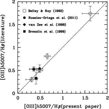
Figure 3: Comparison between redding-corrected fluxes [O iii]$\lambda$5007/H$\beta$ obtained in the present paper and data from the literature (Belley & Roy, 1992; Rosales-Ortega et al., 2011; van Zee et al., 1998; Bresolin et al., 1999) for common H ii regions.

2.3 Comparison with previous observations

H ii regions in the galaxies NGC 628 and NGC 7331 have previously been observed via spectroscopy (McCall et al., 1985; Ferguson et al., 1998; van Zee et al., 1998; Bresolin et al., 1999) or the spectrophotometric imaging (Belley & Roy, 1992) or the Integral Field Spectroscopy method (Rosales-Ortega et al., 2011). There is only one overlapping with the previous spectroscopic observations in every galaxy: one object in NGC 628 observed by van Zee et al. (1998) and one object in NGC 7331 observed by Bresolin et al. (1999). In Fig. 3 we compared our measurements with results of these two previous spectroscopic observations, with results of the spectrophotometric imaging (Belley & Roy, 1992), which are not as accurate as spectroscopic ones for individual objects, and with results of the Integral Field Spectroscopy for NGC 628 (one object (Rosales-Ortega et al., 2011)) (see Table 3).

Fig. 3 shows a satisfactory agreement between our spectroscopy and previous observations. Note that for the quantitative analysis more statistics is necessary. Previous spectroscopic observations of H ii regions in NGC 628 and NGC 7331 will be also compared in Section 3 via radial oxygen and nitrogen abundances distributions in disks of parent galaxies.

3 Abundances

Here we use the spectral data, presented in Section 2 for the determination of the oxygen and nitrogen abundances (and electron temperatures) in H ii regions aiming to establish the radial distributions of these elements across the disks of galaxies.

3.1 Preliminary remarks

Since our measurements of the [N ii]$\lambda$6584 and [O iii]$\lambda$5007 lines are more reliable than those of the [N ii]$\lambda$6548 and [O iii]$\lambda$4959 lines, we used [N ii]$\lambda$6584 and [O iii]$\lambda$5007 lines only. The [O iii]$\lambda$5007 and $\lambda$4959 lines originate from transitions from the same energy level, so their fluxes ratio is due only to the transition probability ratio which is 3.013 (Storey & Zeippen, 2000). Hence, the value of $R_{3}$ can be well approximated by

$$R_{3}=1.33\;I_{\rm{\rm[OIII]}\lambda 5007}/I_{\rm{\rm H}\beta}.$$ (5)

Similarly, the [N ii]$\lambda$6584 and $\lambda$6548 lines also originate from transitions from the same energy level and the transition probability ratio for those lines is 3.071 (Storey & Zeippen, 2000). The value of $N_{2}$ is therefore well approximated by

$$N_{2}=1.33\;I_{\rm\rm[NII]\lambda 6584}/I_{\rm{\rm H}\beta}.$$ (6)

We have used Eq.(6) instead of Eq.(2) to obtain the value of $N_{2}$ and Eq.(5) instead of Eq.(4) to determine the value of $R_{3}$.

The intensities of strong, easily measured lines can be used to separate different types of emission-line objects according to their main excitation mechanism. Baldwin, Phillips & Terlevich (1981) proposed a diagram (BPT classification diagram) where the excitation properties of H ii regions are studied by plotting the low-excitation [N ii]$\lambda$6584/H$\alpha$ line ratio against the high-excitation [O iii]$\lambda$5007/H$\beta$ line ratio.

The [N ii]$\lambda$6584/H$\alpha$ versus [O iii]$\lambda$5007/H$\beta$ diagram is shown in Fig. 4. The symbols are H ii regions. The solid line represents the relation

$$\log(\mbox{\rm[O\,{\sc iii}]$\lambda$5007/H$\beta$})=\frac{0.61}{\log(\mbox{\rm[[N\,{\sc ii}]$\lambda$6584/H$\alpha$})-0.05}+1.3,$$ (7)

which separates objects with H ii spectra from those containing an AGN (Kauffmann et al., 2003). The dashed separation line is the relation

$$\log(\mbox{\rm[O\,{\sc iii}]$\lambda$5007/H$\beta$})=\frac{0.61}{\log(\mbox{\rm[[N\,{\sc ii}]$\lambda$6584/H$\alpha$})-0.47}+1.19$$ (8)

from Kewley et al. (2001). Fig. 4 shows that all H ii regions from our sample are thermally photoionised objects if the separation line from Kewley et al. (2001) is used. When the separation line from Kauffmann et al. (2003) is used then one object (No. 7 in NGC 783) has an appreciable shift from the separation line towards the AGNs. However the uncertainty in the measurement of the intensity of the [N ii]$\lambda$6584 line is large for this object (see Table 4). Therefore all H ii regions are included in further consideration. The abundances determined for object No. 7 from NGC 783 are not considered in question.

Figure 4: The [N ii]$\lambda$6584/H$\alpha$ versus [O iii]$\lambda$5007/H$\beta$ diagram. The symbols are the H ii regions. The solid line separates objects with H ii spectra from those containing an AGN according to Kauffmann et al. (2003). The dashed line is the separation line from Kewley et al. (2001).

3.2 Abundances and temperatures

Accurate oxygen and nitrogen abundances in H ii regions can be derived via the classic $T_{e}$ method, often referred to as the direct method. This method is based on the measurement of the electron temperature $t_{3}$ within the [O iii] zone and/or the electron temperature $t_{2}$ within the [O ii] zone. The ratio of the nebular to auroral oxygen line intensities [O iii]($\lambda$4959+$\lambda$5007)/[O iii]$\lambda 4363$ is usually used for the $t_{3}$ determination, while the ratios of the nebular to auroral nitrogen line intensities [N ii]($\lambda 6548+\lambda 6584$)/[N ii]$\lambda 5755$ or [O ii]($\lambda 3727+\lambda 3729$)/[O ii]($\lambda 7320+\lambda 7330$) are used for the $t_{2}$ determination. The auroral lines in spectra of H ii regions from our sample are too faint to be detected. In this case, it is still possible to obtain the estimates of the nebular abundances, using intensity ratios of the brightest ionic emission lines.

Pagel et al. (1979) and Alloin et al. (1979) have suggested that the locations of H ii regions in some emission-line diagrams can be calibrated in terms of their oxygen abundances. This approach to abundance determination in H ii regions, usually referred to as the ”strong line method” has been widely adopted, especially in the cases where the temperature-sensitive auroral lines are not detected. Numerous relations have been proposed to convert metallicity-sensitive emission-line ratios into metallicity or temperature estimates (e.g. Dopita & Evans, 1986; Zaritsky et al., 1994; Vilchez & Esteban, 1996; Pilyugin, 2000, 2001; Pettini & Pagel, 2004; Tremonti et al., 2004; Pilyugin & Thuan, 2005; Liang et al., 2006; Stasińska, 2006; Thuan et al., 2010). (See the review in Ellison et al. (2008); López-Sánchez & Esteban (2010) for more details).

Two calibration relations for estimation of the oxygen and nitrogen abundances H ii regions have been recently suggested. The ON-calibration relations give the oxygen and nitrogen abundances and electron temperature in terms of the fluxes of the strong emission lines O⁺⁺, O⁺, and N⁺ (Pilyugin et al., 2010). The NS-calibration relations give abundances and electron temperatures in terms of the fluxes in the strong emission lines of O⁺⁺, N⁺, and S⁺ (Pilyugin & Mattsson, 2011). The ON and NS calibrations provide reliable oxygen and nitrogen abundances for H ii regions of all metallicities. The oxygen $R_{2}$ line is measured in presented spectra with a large uncertainty (or even not available). Therefore we use the NS calibration method to estimate the abundances and electron temperatures in our sample of H ii regions.

Table 5: Oxygen and nitrogen abundances and electron temperatures $t_{2}$ in H ii regions derived using the NS calibrations.

H ii region	RGa	12+log(O/H)NS	12+log(N/H)NS	tNSb
NGC 628
4	0.25	8.36	7.16	0.77
7	0.37	8.58	7.79	0.74
8	0.48	8.55	7.70	0.77
9	0.49	8.56	7.57	0.82
10	0.57	8.56	7.64	0.75
NGC 783
1	0.73	8.42	7.57	0.88
3	0.57	8.56	7.90	0.71
4	0.82	8.46	7.65	0.81
6	0.77	8.46	7.74	0.79
7	0.84	8.34	7.61	0.91
8	0.58	8.57	7.91	0.72
NGC 2336
1a	0.88	8.47	7.61	0.81
1b	0.88	8.38	7.32	0.91
2	0.72	8.56	7.75	0.75
3	0.48	8.66	7.92	0.68
6	0.98	8.40	7.18	0.88
7a	0.65	8.54	7.69	0.76
7b	0.65	8.59	7.80	0.71
8	0.55	8.68	7.83	0.66
9	0.44	8.78	8.09	0.59
10a	0.50	8.63	7.90	0.68
10b	0.50	8.63	7.92	0.68
11	0.45	8.47	7.63	0.80
13	0.63	8.58	7.87	0.72
14a	0.97	8.43	7.43	0.88
14b	0.97	8.44	7.41	0.87
15b	0.79	8.47	7.43	0.84
16a	0.52	8.59	7.63	0.73
16b	0.52	8.64	7.76	0.69
17a	0.60	8.59	7.80	0.71
17b	0.60	8.57	7.92	0.72
19	0.56	8.62	7.66	0.71
20	0.62	8.57	7.81	0.72
21	0.57	8.52	7.94	0.74
22	0.76	8.54	7.69	0.76
23	0.74	8.52	7.68	0.78
24	0.66	8.44	7.57	0.84
25	0.65	8.48	7.59	0.82
26	0.53	8.50	7.69	0.78
27	0.55	8.47	7.61	0.81
28	0.86	8.50	7.64	0.79
NGC 6217
1	0.48	8.65	7.89	0.68
3	0.47	8.46	7.65	0.83
NGC 7331
1	0.49	8.44	7.59	0.85
3	0.17	8.41	7.39	0.69
4	0.45	8.53	7.71	0.76
NGC 7678
1	0.90	8.45	7.42	0.87
2	0.59	8.51	7.67	0.78
3	0.56	8.30	6.98	0.80
4	0.56	8.55	7.67	0.76
5	0.56	8.52	7.92	0.75
6	0.49	8.55	7.71	0.74
7	0.67	8.49	7.58	0.80
8a	0.59	8.53	7.66	0.77
8b	0.59	8.54	7.74	0.76

Table 5: Continued

H ii region	RGa	12+log(O/H)NS	12+log(N/H)NS	tNSb
9	0.82	8.51	7.75	0.78
10	0.38	8.52	7.63	0.77

^a in unit of isophotal radius $R_{25}$.

^b $t_{2}$ in unit of 10⁴ K.

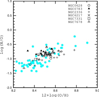
Figure 5: The O/H–N/O diagram. The different symbols marked in the legend show abundances derived using the NS-calibration for our sample of H ii regions. The filled circles show $T_{e}$-based abundances in the sample of best-studied H ii regions in nearby galaxies (the compilation of data from Pilyugin et al. (2010)).

Both individual H ii regions, excited by a single sourse (single star or star cluster), and giant H ii regions can be observed in nearby galaxies. Giant H ii regions can be composite nebulae which contain a number of H ii regions with different physical properties, all contributing to the global spectrum (Kennicutt, 1984). The ON and NS calibrations give oxygen and nitrogen abundances in composite nebulae which agree with the mean luminosity-weighted abundances of their components to within $\sim$0.2 dex (Pilyugin et al., 2012).

The calibrations are constructed under the assumption that the H ii regions are in the low-density regime. Since the sulphur lines [S ii]$\lambda$6717 and [S ii]$\lambda$6731 in most of our spectra are blended (the [S ii]$\lambda$6717 and [S ii]$\lambda$6731 were deblended in a several cases only and with a low accuracy), we cannot estimate the density sensitive ratio [S ii]$\lambda$6717/[S ii]$\lambda$6731 and verify the low-density regime in our objects. Therefore we assume that the H ii regions of our sample are all in the low-density regime, which is typical for the majority of extragalactic H ii regions (Zaritsky et al., 1994; Bresolin et al., 2005; Gutiérrez & Beckman, 2010).

In previous works, a little attention was paid to the radial distribution of nitrogen abundances in the disks of spiral galaxies, despite the fact that such studies would have several advantages (Thuan et al., 2010). First, since at $12+\log$(O/H) $\ga 8.3$, secondary nitrogen becomes dominant and the nitrogen abundance increases at a faster rate than the oxygen abundance (Henry et al., 2000), the change in nitrogen abundances with galactocentric distance should show a larger amplitude in comparison to oxygen abundances and, as a consequence, the gradient (and differences in gradients among galaxies) should be easier to detect. Furthermore, there is a time delay in the nitrogen production as compared to oxygen production (Maeder, 1992; van den Hoek & Groenewegen, 1997; Pagel, 1997; Pilyugin & Thuan, 2011). This provides an additional constraint on the chemical evolution of galaxies. For these reasons, not only the radial distribution of oxygen abundances but also that of nitrogen abundances are estimated here.

The resultant NS calibration abundances and electron temperatures are given in Table 5. The oxygen and nitrogen abundances and electron temperature were derived for H ii regions where $R_{3}$, $N_{2}$, and $S_{2}$ lines are available. It should be noted that the NS-calibration relations have been derived using spectra of H ii regions with well-measured electron temperatures as calibration datapoints. Therefore, the NS-calibration relations produce the abundances which are in agreement with the abundance scale defined by the classic $T_{\rm e}$ method.

Figure 6: Radial distributions of oxygen abundances (left column panels) and nitrogen abundances (right column panels) in the disks of galaxies. Filled circles are abundances estimated from our observational data, open circles are abundances based on the line measurements from the literature. The solid lines are best fits to these datapoints.

The O/H–N/O diagram gives a possibility to test the validity of the determined abundances. On the O/H–N/O diagram (Fig. 5) we compare abundances of 50 H ii regions in six studied galaxies (see legend) with $T_{e}$-based abundances of the best studied H ii regions (open circles) in nearby galaxies (data compiled from Pilyugin et al. (2010)). One can see from Fig. 5, that all points lie within the spread of Pilyugin et al. (2010), i.e. the abundances in our sample of H ii regions derived using the NS-calibration occupy the same band in the O/H - N/O diagram as the $T_{e}$-based abundances in the sample of best-studied H ii regions in nearby galaxies. This shows that our abundance estimations based on the NS-calibration method are realistic.

3.3 Radial abundance gradients

It is common practice (e.g. Zaritsky et al., 1994; van Zee et al., 1998; Pilyugin et al., 2004) that the radial oxygen abundance distribution in the disk of spiral galaxy is fitted by the expression of the type:

$$12+\log({\rm O/H})=12+\log({\rm O/H})_{0}+C_{\rm O/H}\times(R/R_{25}),$$ (9)

where 12 + log(O/H)₀ is the extrapolated central oxygen abundance, $C_{\rm O/H}$ is the slope of the oxygen abundance gradient expressed in terms of dex/$R_{\rm 25}$, and $R$/$R_{\rm 25}$ is the fractional radius (the galactocentric distance normalized to the disk isophotal radius). Analogously to the case of the oxygen abundance, the radial nitrogen abundance distribution in the disk of spiral galaxy is fitted by the equation of the type:

$$12+\log({\rm N/H})=12+\log({\rm N/H})_{0}+C_{\rm N/H}\times(R/R_{25}).$$ (10)

Fig. 6 shows the radial oxygen (left column of panels) and nitrogen (right column of panels) abundances distributions in the disk of spiral galaxies NGC 628, NGC 783, NGC 2336, NGC 7331, and NGC 7678. The abundances derived from our spectral data are shown by the filled circles.

The emission line measurements in the spectra of H ii regions in the disk of the galaxy NGC 628 previously were reported by McCall et al. (1985); Ferguson et al. (1998); van Zee et al. (1998); Bresolin et al. (1999) and in the disk of the galaxy NGC 7331 were given by McCall et al. (1985); Ferguson et al. (1998).

As noted in Section 2.3, there are only two objects in NGC 628 and NGC 7331 in common with previous spectroscopic observations. Nevertheless the abundances estimations in NGC 628 and NGC 7331 can be directly compared with previously published ones. First we estimated the oxygen and nitrogen abundances through the NS calibration, using previously published line measurements. Further, we plotted these estimations on the diagram of the radial distributions of oxygen and nitrogen abundances in the disks of NGC 628 and NGC 7331 together with our abundances estimations.

The galactocentric distances were recomputed with the inclinations and position angles adopted here (Table 1).

Fig. 6 shows a good agreement in the radial abundances distribution in NGC 628 and NGC 7331 between H ii regions observed in present paper (filled circles) and H ii regions observed previously (open circles) in these galaxies.

Table 6: Parameters of radial distributions of oxygen and nitrogen abundances in the disks of galaxies.

galaxy	O/H	O/H	N/H	N/H
	centera	gradientb	centera	gradientb
NGC 628	8.74 $\pm$0.02	-0.43 $\pm$0.03	8.26 $\pm$0.05	-1.34 $\pm$0.08
NGC 783	8.94 $\pm$0.12	-0.65 $\pm$0.16	8.49 $\pm$0.19	-1.07 $\pm$0.26
NGC 2336	8.79 $\pm$0.05	-0.38 $\pm$0.07	8.25 $\pm$0.10	-0.90 $\pm$0.15
NGC 7331	8.75 $\pm$0.18	-0.49 $\pm$0.36	8.23 $\pm$0.36	-1.03 $\pm$0.74
NGC 7678	8.61 $\pm$0.03	-0.15 $\pm$0.05	7.89 $\pm$0.17	-0.34 $\pm$0.27

^a in unit of 12+log(X/H).

^b in unit of dex/$R_{25}$.

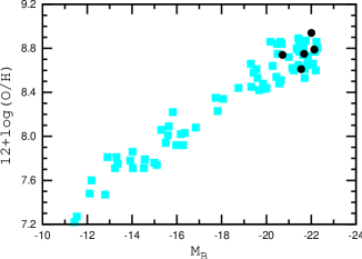
Figure 7: The luminosity – central metallicity diagram. The dark (black) circles denote the central abundances in the disks of spiral galaxies from the present sample. The grey (blue) squares show the central abundances in the disks of spiral galaxies and abundances in irregular galaxies from Pilyugin et al. (2007). (A colour version of this figure is available in the online version.)

The numerical values of the coefficients in Eq.(9) ($C_{\rm O/H}$ and 12 + log(O/H)₀) and in Eq.(10) ($C_{\rm N/H}$ and 12 + log(N/H)₀) have been derived through the least squares method. Both our data and data from the literature are used. If there are datapoints which deviate significantly (more than 3$\sigma$) from the general trend, then these points were excluded in the derivation of the final relations. The obtained relations are presented on the Fig. 6 by the solid lines. Computed parameters of radial distributions of oxygen and nitrogen abundances (the numerical values of the coefficients in Eq.(9) and Eq.(10)) in the disks of galaxies NGC 628, NGC 783, NGC 2336, NGC 7331, and NGC 7678 are listed in Table 6.

3.4 Discussion

Examination of Fig. 6 shows that the radial distributions of the oxygen and nitrogen abundances in the disks of considered galaxies are fitted well by the single linear expression within the optical isophotal radius. The variation of nitrogen abundances with galactocentric distance shows a larger amplitude in comparison to oxygen abundances and the differences in nitrogen abundance gradients among galaxies are larger than that in oxygen abundance gradients.

The luminosity – central metallicity diagram for spiral and irregular galaxies have been constructed in Pilyugin et al. (2007). The abundances of H ii regions in that paper and here have been estimated through the methods producing the abundances which are in agreement with the abundance scale defined by the classic $T_{\rm e}$ method. Therefore the abundances obtained in these studies can be compared. Fig. 7 shows the luminosity – central metallicity diagram. The grey (blue) squares show the central abundances in the disks of spiral galaxies and abundances in irregular galaxies from Pilyugin et al. (2007). The dark (black) circles denote the central abundances in the disks of spiral galaxies from the present sample. The absolute blue magnitudes $M_{B}$ are taken from the leda data base. Inspection of Fig. 7 shows that our sample of galaxies follows well the general trend in the luminosity – central metallicity diagram for spiral and irregular galaxies.

4 Conclusions

The spectroscopic observations of H ii regions in six spiral galaxies (NGC 628, NGC 783, NGC 2336, NGC 6217, NGC 7331, and NGC 7678) obtained with the 6-meter telescope of Special Astrophysical Obsevatory (SAO) of the Russian Academy of Sciences were carried out.

The oxygen and nitrogen abundances as well the electron temperatures in 50 H ii regions are estimated using the recent version of the strong line method (the NS-calibration). The parameters of the radial distributions (the extrapolated central intercept value and the gradient) of the oxygen and nitrogen abundances in the disks of the NGC 628, NGC 783, NGC 2336 and NGC 7678 are obtained. The oxygen and nitrogen abundances and their gradients in the disks of spiral galaxies NGC 783, NGC 2336, and NGC 7678 are estimated for the first time. The abundances for the NGC 6217 are also found for the first time.

Galaxies from our sample follow well the general trend in the luminosity – central metallicity diagram for spiral and irregular galaxies.

References

- Afanasiev & Moiseev (2005) Afanasiev L.V., Moiseev A.V. 2005, Astron. Lett., 31, 193
- Alloin et al. (1979) Alloin D., Collin-Souffrin S., Joly M., Vigroux L. 1979, A&A, 78, 200
- Artamonov et al. (1999) Artamonov B.P., Badan Yu.Yu., Bruyevich V.V., Gusev A.S. 1999, Astron. Rep., 43, 377
- Artamonov et al. (1997) Artamonov B.P., Bruevich V.V., Gusev A.S. 1997, Astron. Rep., 41, 577
- Baldwin, Phillips & Terlevich (1981) Baldwin J.A., Phillips M.M., Terlevich R. 1981, PASP, 93, 5
- Belley & Roy (1992) Belley J., Roy J.-R. 1992, ApJS, 78, 61
- Bresolin et al. (1999) Bresolin F., Kennicutt R.C., Garnett D.R. 1999, ApJ, 510, 104
- Bresolin et al. (2005) Bresolin F., Schaerer D., Conzález Delgado R.M., Stasińska G. 2005, A&A, 441, 981
- Bresolin et al. (2009) Bresolin F., Gieren W., Kudritzki R.-P., Pietrzyński G., Urbaneja M.A., Carraro G. 2009, ApJ, 700, 309
- Bruevich et al. (2007) Bruevich V.V., Gusev A.S., Ezhkova O.V., Sakhibov F.Kh., Smirnov M.A. 2007, Astron. Rep., 51, 222
- Chiappini et al. (2003) Chiappini V., Romano D., Matteucci F. 2003, MNRAS, 339, 63
- Dinerstein (1990) Dinerstein H.L. 1990, in ”The Interstellar Medium in Galaxies” eds. H.A. Thronson (Jr.) and J.M. Shull (Dordrecht: Kluwer), 257
- Dopita & Evans (1986) Dopita M.A., Evans I.N. 1986, ApJ, 307, 431
- Dutil & Roy (1999) Dutil D.R., Roy J.-R. 1999, ApJ, 516, 62
- Ellison et al. (2008) Ellison S.L., Patton D.R., Simard L., McConnachie A.W. 2008, AJ, 135, 1877
- Ferguson et al. (1998) Ferguson A.M.N., Gallagher J.S., Wyse R.F.G. 1998, AJ, 116, 673
- Garnett & Shields (1987) Garnett D.R., Shields G.A. 1987, ApJ, 317, 82
- Garnett (2002) Garnett D.R. 2002, ApJ, 581, 1019
- Gusev (2006a) Gusev A.S. 2006a, Astron. Rep., 50, 167
- Gusev (2006b) Gusev A.S. 2006b, Astron. Rep., 50, 182
- Gusev & Park (2003) Gusev A.S., Park M.-G. 2003, A&A, 410, 117
- Gutiérrez & Beckman (2010) Gutiérrez L., Beckman J.E. 2010, ApJ, 710, L44
- Henry et al. (2000) Henry R.B.C., Edmunds M.G., Kóppen J. 2000, ApJ, 541, 660
- Izotov et al. (1994) Izotov Y.I., Thuan T.X., Lipovetsky V.A. 1994, ApJ, 435, 647
- Izotov et al. (2004) Izotov Y.I., Stasińska G., Guseva N.G., Thuan T.X. 2004, A&A, 415, 87
- Kartasheva & Chunakova (1978) Kartasheva T.A., Chunakova N.M. 1978, Izv. SAO, 10, 44
- Kauffmann et al. (2003) Kauffmann G., Heckman T.M., Tremonti C., et al. 2003, MNRAS, 346, 1055
- Kennicutt (1984) Kennicutt R.C. 1984, ApJ, 287, 116
- Kennicutt et al. (2003) Kennicutt R.C., Bresolin F., Garnett D.R. 2003, ApJ, 591, 801
- Kewley et al. (2001) Kewley L.J., Dopita M.A., Sutherland R.S., Heisler C.A., Trevena J. 2001 ApJ, 556, 121
- Liang et al. (2006) Liang Y.C., Yin S.Y., Hammer F., Deng L.C., Flores H., Zhang B. 2006, ApJ, 652, 257
- López-Sánchez & Esteban (2010) López-Sánchez Á.R., Esteban C. 2010, A&A, 517, A85
- Maeder (1992) Maeder A. 1992, A&A, 264, 105
- Marcon-Uchida et al. (2010) Marcon-Uchida M.M., Matteucci F., Costa, R.D.D. 2010, A&A, 520, A35
- McCall et al. (1985) McCall, M. L., Rybski, P. M., Shields, G. A. 1985, ApJS, 57, 1
- Moustakas et al. (2010) Moustakas J., Kennicutt R.C. (Jr), Tremonti C.A., Dale D.A., Smith J.-D.T., Calzetti D. 2010, ApJS, 190, 233
- Oke (1990) Oke J.B. 1990, AJ, 99, 1621
- Osterbrock (1989) Osterbrock D.E. 1989, Astrophysics of gaseous nebulae and active galactic nuclei (Mill Valley, CA: University Science Books), 422 p.
- Pagel et al. (1979) Pagel B. E. J., Edmunds M. G., Blackwell D. E., Chun M. S., Smith G. 1979, MNRAS, 189, 95
- Pagel (1991) Pagel B.E.J. 1991, Nuclei in the Cosmos, ed. H. Oberhummer (Berlin: Springer), 89
- Pagel (1997) Pagel B.E.J., 1997, Nucleosynthesis and Chemical Evolution of Galaxies (Cambridge: Cambridge Univ. Press), 392 p.
- Paturel at al. (2003) Paturel G., Petit C., Prugniel Ph., Theureau G., Rousseau J., Brouty M., Dubois P., Cambresy L. 2003, A&A, 412, 45
- Pettini & Pagel (2004) Pettini, M., Pagel, B.E.J. 2004, MNRAS, 348, 59L
- Pilyugin (2000) Pilyugin L.S. 2000, A&A, 362, 325
- Pilyugin (2001) Pilyugin L.S. 2001, A&A, 369, 594
- Pilyugin et al. (2004) Pilyugin L.S., Vílchez J.M., Contini T. 2004, A&A, 425, 849
- Pilyugin & Thuan (2005) Pilyugin L.S., Thuan T.X. 2005, ApJ, 631, 231
- Pilyugin et al. (2007) Pilyugin L.S., Thuan T.X., Vílchez J.M. 2007, MNRAS, 376, 353
- Pilyugin et al. (2010) Pilyugin L.S., Vílchez J.M., Thuan T.X. 2010, ApJ, 720, 1738
- Pilyugin & Thuan (2011) Pilyugin L.S., Thuan T.X. 2011, ApJ, 726, L23
- Pilyugin & Mattsson (2011) Pilyugin L.S., Mattsson L. 2011, MNRAS, 412, 1145
- Pilyugin et al. (2012) Pilyugin L.S., Vílchez J.M., Mattsson L., Thuan T.X. 2012, MNRAS, 421, 1624
- Rosales-Ortega et al. (2011) Rosales-Ortega F.F., Diaz A.I., Kennicutt R.C., Sanchez S.F. 2011, MNRAS, 415, 2439
- Roy et al. (1996) Roy J.-R., Belley J., Dutil Y., Martin P. 1996, ApJ, 460, 294
- Searle (1971) Searle L. 1971, ApJ, 168, 327
- Stasińska (2006) Stasińska G. 2006, A&A, 454, L127
- Storey & Zeippen (2000) Storey P.J., Zeippen C.J. 2000, MNRAS, 312, 813
- Thuan et al. (2010) Thuan T.X., Pilyugin L.S., Zinchenko I.A. 2010, ApJ, 712, 1029
- Tremonti et al. (2004) Tremonti C.A., Heckman T.M., Kauffmann G., et al. 2004, ApJ, 613, 898
- van den Hoek & Groenewegen (1997) van den Hoek L.B., Groenewegen M.A.T. 1997, A&AS, 123, 305
- van Zee et al. (1998) van Zee L., Salzer J.J., Haynes M.P., O’Donoghue A.A., Balonek T.J. 1998, AJ, 116, 2805
- Vila-Costas & Edmunds (1992) Vila-Costas M.B., Edmunds M.G. 1992, MNRAS, 259, 121
- Vilchez & Esteban (1996) Vilchez J.M., Esteban C. 1996, MNRAS, 280, 720
- Zaritsky et al. (1994) Zaritsky D., Kennicutt R.C., Huchra J.P. 1994, ApJ, 420, 87