Relativistic jet models for two low-luminosity radio galaxies: evidence for backflow?

Abstract

We show that asymmetries in total intensity and linear polarization between the radio jets and counter-jets in two lobed Fanaroff-Riley Class I (FR I) radio galaxies, B2 0206+35 (UGC 1651) and B2 0755+37 (NGC 2484), can be accounted for if these jets are intrinsically symmetrical, with decelerating relativistic outflows surrounded by mildly relativistic backflows. Our interpretation is motivated by sensitive, well-resolved Very Large Array imaging which shows that both jets in both sources have a two-component structure transverse to their axes. Close to the jet axis, a centrally-darkened counter-jet lies opposite a centrally-brightened jet, but both are surrounded by broader collimated emission that is brighter on the counter-jet side. We have adapted our previous models of FR I jets as relativistic outflows to include an added component of symmetric backflow. We find that the observed radio emission, after subtracting contributions from the extended lobes, is well described by models in which decelerating outflows with parameters similar to those derived for jets in plumed FR I sources are surrounded by backflows containing predominantly toroidal magnetic fields. These return to within a few kpc of the galaxies with velocities $\approx 0.25c$ and radiate with a synchrotron spectral index $\alpha\approx 0.55$. We discuss whether such backflow is to be expected in lobed FR I sources and suggest ways in which our hypothesis can be tested by further observations.

1 Introduction

Relativistic jet outflows from radio galaxies are a primary mechanism for energy extraction from supermassive black holes in active galactic nuclei (AGN) and an important source of energy input to the intergalactic medium (IGM) in groups and clusters (e.g. McNamara & Nulsen 2007, and references therein). We are studying relativistic jet kinematics and dynamics in nearby low-luminosity radio galaxies with Fanaroff-Riley Class I (FR I - Fanaroff & Riley 1974) morphology for which we have obtained radio imaging and polarimetry at high angular resolution transverse to the jets as well as along their lengths. We have developed procedures for deriving three-dimensional variations of intrinsic jet parameters – velocity field, emissivity and magnetic-field ordering – from an analysis of systematic asymmetries between the jets and counter-jets (Laing & Bridle, 2002a; Canvin & Laing, 2004; Canvin et al., 2005; Laing et al., 2006a). We compare the observed asymmetries in images of total intensity, degree of linear polarization and apparent magnetic field direction with the predicted effects of relativistic aberration on synchrotron emission from particles in partially-ordered magnetic fields in model outflows and deduce the distributions of intrinsic properties within the jets. We have found that a generic property of the jet outflows in FR I radio galaxies is that they decelerate from relativistic speeds ($\beta=v/c\approx 0.8$ – 0.9) near the AGN to subrelativistic speeds a few kiloparsecs away, and that the outflows are systematically faster on-axis than at their edges.

It is critical for such an analysis to distinguish patterns of asymmetry in the jets produced by relativistic aberration from any that are intrinsic to the outflows or which result from interactions between the outflows and anisotropic environments, e.g. from pressure gradients or winds in the IGM. One asymmetry in FR I radio jets that has proven instructive in some sources and problematic in others is the systematic difference between transverse intensity profiles in the brighter jets and weaker counter-jets when observed at high sensitivity and angular resolution.

This difference correlates with indicators of the orientation of the jets to the line of sight. A statistical study of FR I jets in the B2 sample by Laing et al. (1999) found that the ratio of jet to counter-jet FWHM measured by Gaussian fitting at the same distance from the nucleus on both sides is strongly anticorrelated with the average jet/counter-jet brightness ratio and with the ratio of core to extended flux density.

This anticorrelation is qualitatively as expected for intrinsically symmetrical relativistic outflows which are faster on-axis than at their edges. In this case, relativistic aberration makes the transverse brightness profiles of the approaching, hence apparently brighter, jet more centrally peaked than those of the receding counter-jet. Gaussian fitting to the jet and counter-jet FWHM then yields smaller values of the width for the apparently brighter jets even if the (slower moving) outer boundaries of the jets appear identical on both sides of the AGN.

The amplitude of the effect found in the B2 source sample by Laing et al. (1999) is, however, surprisingly large. Modelling of the anticorrelation requires that the velocity $\beta_{\rm on-axis}\approx 0.7$ and $\beta_{\rm edge}\approx 0.1$ (Laing et al., 1999) in order to reproduce the spread of width ratios. Two lines of argument suggest that such large velocity ratios are not typical of the FR I population. Firstly, the ratio $\beta_{\rm edge}/\beta_{\rm on-axis}$ required to explain the effect is quantitatively inconsistent with the brightness and polarization distributions in four of the five individual FR I sources we have modelled (Laing & Bridle 2002a; Canvin & Laing 2004; Canvin et al. 2005 – the exception is 3C 296; Laing et al. 2006a). Secondly, the smallest values of $\beta_{\rm edge}/\beta_{\rm on-axis}$ are required only to generate the unusually small values of jet/counter-jet width ratio $\approx 0.6$ in a few members of the B2 source sample with particularly high jet/counter-jet brightness ratios, whose jets are thought to be highly inclined to the plane of the sky (Laing et al., 1999).

Thus far, our results would be consistent with the idea that all FR I jets are symmetrical outflows, but that only a few have very large transverse velocity gradients. Even this hypothesis fails for two of the B2 sample members, B2 0206+35 and B2 0755+37 (Laing et al., 2011). These sources are unusual in that the lower isophotes of their brighter jets also appear narrower than those of the counter-jets at the same distance from the AGN in images of moderate resolution and sensitivity (e.g. Bondi et al. 2000) - even though the jets clearly exhibit the basal asymmetries associated with symmetrical decelerating relativistic outflows. Apparent width asymmetry in the fainter jet emission cannot generally be explained by relativistic effects alone if the jets are both symmetrical and purely outflowing. On the other hand, if the asymmetry is attributed to intrinsic or environmental differences on the two sides of the AGN (e.g. Bondi et al. 2000) there should be no systematic trend for the wider jet to be on the receding side as it is in the (albeit small) sample of Laing et al. (1999).

In this paper, we explore an alternative explanation for the transverse brightness profile asymmetries of the jets and counter-jets in 0206+35 and 0755+37. This work was motivated by new deep imaging of these sources showing: (a) that their counter-jets have minima in their emission profiles with the same widths as the main jets at similar distances from the nucleus and (b) that the main jets are surrounded by faint emission resembling the broader outer emission in the counter-jets (Laing et al., 2011, and Section 2.2, below). The new imaging data lead us to model the jets in these sources as intrinsically symmetrical outflows near the jet axis surrounded by broader features from backflowing material. If backflow in the broader features can be approximately symmetrical and mildly relativistic, then aberration can make its emission appear slightly brighter on the counter-jet side, producing differences in isophotal width between the jets similar to those observed.

Backflow is a reasonable hypothesis a priori for FR I sources like 0206+35 and 0755+37 whose jets appear to propagate within well-defined lobes. It has been an acknowledged ingredient of models of lobed FR II sources since the first attempts to simulate their hydrodynamics (Norman et al., 1982). FR I sources cannot form lobes without similar deflection of jet material and Laing et al. (2011) showed that FR I lobes resemble those of FR II sources in many respects. If FR I jets are much lighter than their surroundings and initially fast (e.g. Laing & Bridle 2002b), we should not be surprised if some large-scale post-jet flow in FR I lobes is marginally relativistic. We also note that mildly relativistic backflow extends almost all the way back to the centre of the host galaxy in simulations of relativistic FR I jets with initial dynamical flow parameters matching those deduced from our observations of 3C 31 and realistic pressure and density profiles for the surrounding IGM (Laing & Bridle, 2002b; Perucho & Martí, 2007).

In this paper, we show that a fully symmetrical model in which a decelerating axisymmetric outflow is surrounded by a slower (but still slightly relativistic) backflow is quantitatively consistent with the detailed brightness and polarization distributions of the jets and counter-jets in 0206+35 and 0755+37. It is not obvious a priori that conditions needed to produce symmetrical backflow are likely to be realised in lobed FR I radio galaxies. Nevertheless, our results suggest that mildly relativistic backflow contributes significantly to the observed jet vs counter-jet width relationships and we suggest ways in which this (perhaps unexpected) ingredient of FR I source structure could be investigated further.

In Section 2, we summarize the optical and large-scale radio properties of the sources and discuss the additional image processing required to separate jet and lobe emission. Section 3 describes our modelling procedure and Section 4 gives a comparison between models and data. The model parameters are presented in Section 5. A brief discussion is given in Section 6. Section 7 summarizes our conclusions and suggests further work. Finally, Appendix A demonstrates that a toroidally-magnetized outflow can, in special circumstances, produce jet/counter-jet sidedness ratios significantly less than unity.

We adopt a concordance cosmology with Hubble constant, $H_{0}$ = 70 $\rm{km\,s^{-1}\,Mpc^{-1}}$, $\Omega_{\Lambda}=0.7$ and $\Omega_{M}=0.3$.

2 Observations and images

2.1 The sources: optical data and large-scale radio structures

The galaxy identifications, redshifts and linear scales for the two sources studied here are given in Table 1. Their radio structures have been described in detail by Laing et al. (2011), from which the images in Fig. 1 are taken.

Table 1: Names, redshifts, linear scales and associated references for the sources in this paper.

Name	Galaxy	Redshift	Scale	Reference
	name		kpc
			arcsec-1
0206+35	UGC 1651	0.03773	0.748	1
0755+37	NGC 2484	0.04284	0.845	2
References: (1) Miller et al. (2002); (2) Falco et al. (1999).

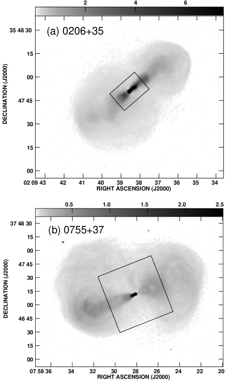
Figure 1: Grey-scale images of the sources (Laing et al., 2011). The boxes mark the areas shown in later plots and the grey-scale ranges, in mJy beam^-1, are indicated by the labelled wedges. (a) 0206+35 at 4.9 GHz, 1.2 arcsec FWHM. (b) 0755+37 at 4.9 GHz, 1.3 arcsec FWHM.

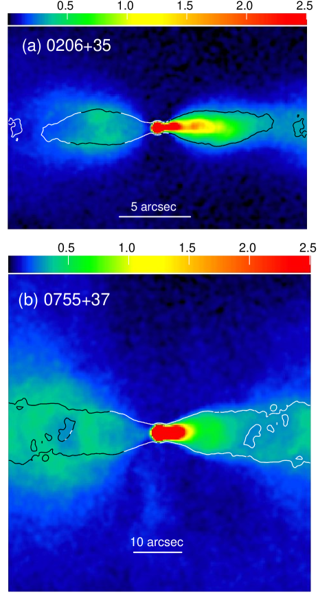
Figure 2: False-colour images of total intensity for 0206+35 and 0755+37 over the areas outlined in Fig. 1. On the right-hand side of each panel, we have plotted a single contour to outline the brightest emission of the main (brighter) jet. On the left-hand side, this contour (rotated through 180°) is plotted on the counter-jet emission. (a) 0206+35 at 0.35-arcsec FWHM resolution. (b) 0755+37 at 1.3-arcsec FWHM resolution.

2.2 Images

Table 2: Parameters of the sub-images used for modelling and spectral analysis. Col. 1: source name; col. 2: observing frequency (an asterisk indicates that the image was used for modelling); col 3: resolution (FWHM); col. 4: rms off-source noise level in $I$; col.5: average noise level in $Q$ and $U$; col. 6: sub-image position angle; col. 7: sub-image sizes parallel and perpendicular to the jet axis.

Source	$\nu$	Res	rms		Rot	Size
	GHz	arc-	$\mu$Jy b-1		deg	arcsec2
		sec	$\sigma_{I}$	$\sigma_{P}$
0206+35	1.425	1.20	19	$-$	$-$41.0	$22\times 20$
0206+35	4.860	1.20	12	$-$	$-$41.0	$22\times 20$
0206+35	4.860	0.35*	7.2	7.1	$-$41.0	$22\times 20$
0755+37	1.425	1.30	20	$-$	158.5	$66\times 66$
0755+37	4.860	1.30*	7.8	7.9	158.5	$66\times 66$
0755+37	4.860	0.40*	8.0	7.1	158.5	$20\times 16$

Table 2 summarizes the relevant parameters of the high-resolution sub-images which we model or use for spectral analysis in this paper (details of the observations and data reduction are given by Laing et al. 2011). The ${\bf E}$-vector position angles of linear polarization at 4.860 GHz have been corrected for Faraday rotation using multifrequency imaging (Guidetti et al., 2011, 2012; Laing et al., 2011) and residual depolarization is predicted to be negligible at this frequency. The areas plotted in later figures are outlined on Fig. 1.

Fig. 2 shows rotated sub-images. On the right-hand side of each panel, we have drawn a single contour to outline the brightest part of the main jet. On the left-hand side, this contour is rotated through 180°and plotted on the counter-jet emission. This diagram emphasizes the points made earlier that the minima in the counter-jet emission have roughly the same widths as the main jets and that the main jets are in turn surrounded by fainter emission.

In order to model jets that appear superimposed on lobes, we must try to separate the two emission components in all Stokes parameters. There is no unique way to do this when their spectra and intensities vary independently across the field of view. Any approach to isolating jet emission in a lobed FR I source therefore entails some simplifying assumption about the variations in intensity $I$ or in spectral index $\alpha$ of the lobes or jets over the region to be modelled. We have attempted to separate the jets and lobes for these sources in a way that optimizes the resolution and signal-to-noise of the jet emission while letting us check for systematic errors resulting from the assumptions made while doing the lobe-jet separation, as follows.

One approach to separating jet and lobe emission observed at two frequencies is based on their systematic spectral differences: the jets have characteristic spectral indices close to $\alpha=0.55$, whereas the lobes have $\alpha\ga 0.8$ near the centres of the sources (Laing et al., 2011). If the spectral index of the lobe emission close to the jet is reasonably constant, we can use a variant of the ‘spectral tomography’ method (Katz-Stone & Rudnick, 1997; Katz-Stone et al., 1999; Laing et al., 2006b) by assuming that what is observed can be described as the sum of two components: a jet and a lobe with constant spectral indices $\alpha_{\rm j}$ and $\alpha_{\rm l}$, respectively. The brightnesses observed at a given point at two frequencies $\nu_{0}$ and $\nu_{1}$ are then:

$$I(\nu_{0}) = B_{\rm j}\nu_{0}^{-\alpha_{\rm j}}+B_{\rm l}\nu_{0}^{-\alpha_{\rm l}}$$

$$I(\nu_{1}) = B_{\rm j}\nu_{1}^{-\alpha_{\rm j}}+B_{\rm l}\nu_{1}^{-\alpha_{\rm l}}$$

We can scale and subtract the two brightness distributions to estimate the jet brightness at the modelling frequency $\nu_{0}$:

$$B_{\rm j}\nu_{0}^{-\alpha_{\rm j}} = \frac{\nu_{0}^{\alpha_{\rm l}}I(\nu_{0})-\nu_{1}^{\alpha_{\rm l}}I(\nu_{1})}{\nu_{0}^{\alpha_{\rm l}}-\nu_{1}^{\alpha_{\rm l}}(\nu_{0}/\nu_{1})^{\alpha_{\rm j}}}$$

Once we know $\alpha_{\rm l}$, the method can also be applied to Stokes $Q$ and $U$ provided that we correct the images at both frequencies for Faraday rotation before subtraction, and that depolarization is negligible (as is the case for these sources). Note that the spectral index of the jets, $\alpha_{\rm j}$, must be both constant and known in order to scale the result correctly.

In practice, we estimated the lobe spectral index for $\nu_{0}=4.860$ GHz and $\nu_{1}=1.425$ GHz by performing the subtraction for various trial values of $\alpha_{\rm l}$ and selecting that which minimized the residual lobe emission in jet-free regions.

Spectral subtraction can remove even rather complicated lobe emission if the spectral index is constant, but it has two serious flaws for our purposes: (a) the signal-to-noise ratio of the corrected image is lower than that of the deep high-frequency image alone and (b) our highest-resolution data for 0206+35 and 0755+37 are only at one frequency.

The alternative of spatial subtraction assumes that the lobe intensity varies only slowly across the jet. This approach can be best applied at high angular resolution where the lobe brightness is low and the spatial variation of jet emission is clearest. To separate the two types of emission spatially in $I$, $Q$ and $U$, we define two background regions parallel to the jet axis and just outside the maximum transverse extent of the jet as estimated from spectral-index images, i.e. using both the intensity and spectral properties of the jet emission to guide our choice of the background regions. We then smooth the background brightness distributions parallel to the jet axis with a boxcar function to improve their signal-to-noise ratio and interpolate linearly between them under the jet. We refer to this approach as generating ‘interpolated images’.

For 0206+35 and 0755+37 we first used spectral subtraction to verify the total extent of the jet emission and to set appropriate reference regions for interpolation, then constructed interpolated images for the final modelling.

Table 3: Interpolation parameters for lobe subtraction. Col. 1: source name; col 2: resolution (FWHM); col. 3: background region distances from jet axis; col. 4: width of boxcar smoothing function parallel to the axis.

Source	FWHM	Background	Smooth
	(arcsec)	(arcsec)	(arcsec)
0206+35	0.35	9 – 10	1.0
0755+37	1.30	30 – 45	3.0

In Figs 3 and 4, we show the results of both subtraction methods for the two sources. Figs 3(a) and 4(a) show the images at the resolution used for modelling before subtraction. We found best-fitting lobe spectral indices between 1.425 and 4.860 GHz of 0.90 and 0.81 for 0206+35 and 0755+37, respectively. In Fig. 3(b), we show the spectral subtraction for 0206+35 at lower resolution. Although not useful for modelling, this image outlines the total extent of the flatter-spectrum emission associated with the jets. The spectral subtraction for 0755+37 at the lower of the two resolutions used for modelling, shown in Fig. 4(b), has little trace of residual lobe emission but low signal-to-noise.

Guided by the spectral subtraction, we set the interpolation parameters as in Table 3 and computed interpolated images at 1.425 and 4.860 GHz, from which we in turn derived the spectral-index images shown in Figs 3(c) and 4(c). These are blanked on the error in spectral index, as noted in the captions. We then estimated integrated spectral indices for the jets by summing the interpolated $I$ images over all pixels which are unblanked on the spectral-index images, excluding the cores. We found $\langle\alpha_{\rm j}\rangle=0.55$ for 0206+35 and 0.53 for 0755+37. We used these values to scale the spectral subtractions. Variations across the modelled regions are small, with $0.50\leq\alpha_{\rm j}\leq 0.62$ in both sources. Finally, we show the 4.860-GHz interpolated images at the resolutions used for modelling in Figs 3(d) and 4(d).

We are confident that the interpolated images represent the jet emission accurately in both sources. The lobe emission in 0206+35 is quite faint at 0.35-arcsec FWHM resolution, and after subtraction, the area around the jets appears devoid of residual emission in all Stokes parameters (e.g. Fig. 3d). The lower-resolution (1.3 arcsec FWHM) image of 0755+37 proved to be more of a challenge, because the lobe emission is bright and irregular (Fig. 4a). The spectral subtraction gave a clean image of the jet with negligible background emission, but amplified noise (Fig. 4b). In contrast, interpolation (Fig. 4d) failed to remove the small-scale lobe emission accurately but retained the full signal-to-noise ratio of our high-frequency images. Comparison of the two corrected $I$ images showed that they are accurately consistent wherever $I>100$ $\mu$Jy beam^-1. We therefore used the interpolated images for modelling (in which the faint residual lobe emission has low weight). Modelling the spectrally-subtracted image (and its counterparts in $Q$ and $U$) gave consistent but less well constrained results. In the intensity and polarization profiles plotted below, we compare the results from both subtraction methods.

At 0.4-arcsec FWHM resolution, used for modelling the inner jets of 0755+37, the lobe brightness is negligible and we did not attempt to subtract it.

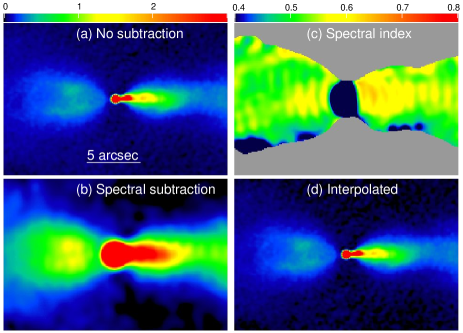
Figure 3: False-colour images showing the results of lobe subtraction for 0206+35. The $I$ intensity colour range (0 – 3 mJy beam^-1) is the same for panels (a) and (d). (a) No subtraction at 0.35-arcsec resolution. (b) Subtraction at 1.2-arcsec resolution assuming a constant spectral index for the lobe. (c) Spectral index distribution over the jet and counter-jet at 1.2-arcsec resolution after interpolated subtraction, blanked where $\sigma_{\alpha}>0.03$ (the colour range for spectral index is shown by the labelled wedge). (d) Subtraction by linear interpolation between background strips parallel to the jet axis. The resolution is 0.35 arcsec.

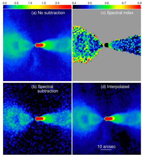
Figure 4: False-colour images showing results of lobe subtraction in 0755+37 at 1.3-arcsec resolution. The $I$ intensity colour range (0 – 2.5 mJy beam^-1) is the same for panels (a), (b) and (d). (a) No subtraction. (b) Subtraction assuming a constant spectral index for the lobe, as described in the text. (c) Spectral index distribution over the jet and counter-jet after interpolated lobe subtraction, blanked where $\sigma_{\alpha}>0.1$ (the colour range for spectral index is indicated by the labelled wedge). (d) Subtraction by linear interpolation between background strips parallel to the jet axis.

3 Model fits

3.1 Assumptions

To model the jet emission, we make the following assumptions.

1. The jets are intrinsically symmetrical, axisymmetric and antiparallel. They can be treated, on average, as laminar, stationary flows.

2. The radio emission is from relativistic particles with a power-law energy spectrum $n(E)=n_{0}E^{-(2\alpha+1)}$ ($\alpha$ is the spectral index). We use the integrated values for the modelled regions after lobe subtraction: $\langle\alpha\rangle=0.55$ for 0206+35 and 0.53 for 0755+37. The corresponding maximum degree of polarization is $p_{0}=(3\alpha+3)/(3\alpha+5)=0.70$ in both cases and the variations of spectral index across the modelled regions are small enough to be ignored (Section 2.2).

3. The magnetic field is tangled on small scales, but anisotropic.

4. The effects of Faraday rotation on the observed emission are corrected completely. This is an extremely good approximation for 0206+35 and 0755+37 (Guidetti et al., 2011, 2012; Laing et al., 2011).

3.2 Outline of method

For a symmetrical, outflowing jet with velocity $v=\beta c$, emitting isotropically in the rest frame and inclined by an angle $\theta$ to the line of sight, a measurement of the observed jet/counter-jet intensity ratio

$$I_{\rm j}/I_{\rm cj} = [(1+\beta\cos\theta)/(1-\beta\cos\theta)]^{2+\alpha}$$

does not allow us to determine the velocity and inclination separately. The key to our method is the use of linear polarization to break this degeneracy. The relation between the angles to the line of sight in the rest frame of the outflow, $\theta^{\prime}$ and in the observed frame, $\theta$, is:

$$\sin\theta^{\prime}_{\rm j} = [\Gamma(1-\beta\cos\theta)]^{-1}\sin\theta\makebox{~{}~{}~{}~{}~{}(main jet)}$$

$$\sin\theta^{\prime}_{\rm cj} = [\Gamma(1+\beta\cos\theta)]^{-1}\sin\theta\makebox{~{}~{}(counter-jet)}$$

The emission in all three Stokes parameters depends on $\theta^{\prime}$, since the magnetic field is in general anisotropic. If the flow is significantly relativistic, we effectively observe the two jets at different values of $\theta^{\prime}$ and can use the differences in polarization for the approaching and receding jets as an additional constraint to separate $\beta$ and $\theta$. For backflow, the argument is identical with the roles of jet and counter-jet interchanged.

The principal steps in our method (Laing & Bridle, 2002a; Canvin & Laing, 2004; Canvin et al., 2005; Laing et al., 2006a) are as follows.

1. Build a parameterized model of the geometry, the velocity field and the variations of emissivity ($\propto n_{0}B^{1+\alpha}$) and magnetic-field anisotropy in the rest frame of the emitting plasma.

2. Calculate the observed-frame emission in $I$, $Q$ and $U$, taking account of relativistic aberration and anisotropic emission in the rest frame.

3. Integrate along the line of sight, normalize to the measured total flux density and convolve with the observing beam.

4. Calculate and sum $\chi^{2}$ over the $I$, $Q$ and $U$ images. This is our measure of goodness of fit.

5. Optimize the parameters using the downhill simplex method of Nelder & Mead (Press et al., 1992).

We explored a wide range of starting simplexes in order to be sure of locating the global minimum in $\chi^{2}$.

3.3 Fitting functions

The parameterized model that we fit to the VLA observations is a simplified version of those in our previous work (Laing & Bridle, 2002a; Canvin & Laing, 2004; Canvin et al., 2005; Laing et al., 2006a), with the addition of a few extra terms to describe the backflow. The functional forms are given explicitly in Table 4. A critical discussion of fitting functions will be given elsewhere (Laing & Bridle, in preparation).

Table 4: Coordinate definitions and functional forms for geometry, velocity, proper emissivity and magnetic-field ordering.

Description	Quantity	Functional form	Distance range
Distance coordinate	$r$	$\frac{zr_{0}}{(r_{0}+A)\cos\xi-A}$	$r\leq r_{0}$
(outflow and backflow)		$\frac{z+A}{\cos\xi}-A$	$r\geq r_{0}$
		$A=x_{0}/\sin\xi_{0}-r_{0}=x_{\rm b}/\sin\xi_{\rm b}-r_{0}$
Outflow streamline index	$s$	by continuity	$r\leq r_{0}$
		$\xi/\xi_{0}$	$r\geq r_{0}$
Outflow radius	$x(z,s)$	$a_{2}(s)z^{2}+a_{3}(s)z^{3}$	$r\leq r_{0}$
		$(z-r_{0}+x_{0}/\sin\xi_{0})\tan(\xi_{0}s)$	$r\geq r_{0}$
Outflow velocity	$\beta(r,s)$	$\beta_{1}\exp(s^{2}\ln v_{1})$	$r\leq r_{v_{1}}$
		$\beta_{1}\exp(s^{2}\ln v_{1})\left(\frac{r_{v0}-r}{r_{v0}-r_{v1}}\right)+\beta_{0}\exp(s^{2}\ln v_{0})\left(\frac{r-r_{v1}}{r_{v0}-r_{v1}}\right)$	$r_{v1}\leq r\leq r_{v0}$
		$\beta_{0}\exp(s^{2}\ln v_{0})$	$r\geq r_{v_{0}}$
Outflow proper emissivity	$\epsilon(r,s)$	$g_{1}r^{-E_{\rm in}}\exp(\ln e_{1}s^{2})$	$r\leq r_{e1}$
		$~{}~{}r^{-E_{\rm mid}}\exp\left[\ln\left(\frac{e_{1}(r_{e0}-r)+e_{0}(r-r_{e1})}{r_{e0}-r_{e1}}\right)s^{2}\right]$	$r_{e1}\leq r\leq r_{e0}$
		$g_{0}r^{-E_{\rm out}}\exp(\ln e_{0}s^{2})$	$r\geq r_{e0}$
Outflow $\langle B_{r}^{2}/B_{t}^{2}\rangle^{1/2}$	$j(r)$	$j_{1}$	$r\leq r_{B1}$
		$\frac{j_{1}(r_{B0}-r)+j_{0}(r-r_{B1})}{r_{B0}-r_{B1}}$	$r_{B1}\leq r\leq r_{B0}$
		$j_{0}$	$r\geq r_{B0}$
Outflow $\langle B_{l}^{2}/B_{t}^{2}\rangle^{1/2}$	$k(r)$	$k_{1}$	$r\leq r_{B1}$
		$\frac{k_{1}(r_{B0}-r)+k_{0}(r-r_{B1})}{r_{B0}-r_{B1}}$	$r_{B1}\leq r\leq r_{B0}$
		$k_{0}$	$r\geq r_{B0}$
Backflow streamline index	$t$	by continuity	$r\leq r_{0}$
		$(\xi-\xi_{0})/(\xi_{\rm b}-\xi_{0})$	$r\geq r_{0}$
Backflow radius	$x(z,t)$	$a_{2}(t)z^{2}+a_{3}(t)z^{3}$	$r\leq r_{0}$
		$(z-r_{0}+x_{0}/\sin\xi_{0})\tan[\xi_{0}+(\xi_{\rm b}-\xi_{0})t]$	$r\geq r_{0}$
Backflow velocity	$\beta(t)$	$\beta_{\rm b,in}+t(\beta_{\rm b,out}-\beta_{\rm b,in})$
Backflow proper emissivity	$\epsilon(r,t)$	0	$r<r_{b}$
		$n_{\rm b}(r/r_{0})^{-E_{\rm b}}\exp(\ln e_{\rm b}t^{2})$	$r\geq r_{b}$
Backflow $\langle B_{r}^{2}/B_{t}^{2}\rangle^{1/2}$	$j$	$j_{\rm b}$
Backflow $\langle B_{l}^{2}/B_{t}^{2}\rangle^{1/2}$	$k$	$k_{\rm b}$

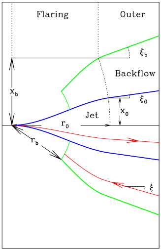
Figure 5: Sketch of the assumed geometry. The blue and green curves show the outer boundaries of the outflowing jet and backflow emission, respectively, Representative streamlines in the two parts of the flow are shown in red. The fiducial distances and angles are defined in Section 3.3.1.

3.3.1 Geometry

We use coordinates $(z,x)$ in a plane containing the jet axis, with $z$ measured along the axis and $x$ perpendicular to it. The jet is divided into a flaring region, where the flow first expands and then recollimates, and a conical outer region, as sketched in Fig. 5. The edge of the outflow is fully defined by the distance of the transition between the two regions measured along the axis, $r_{0}$, the radius, $x_{0}$, and the opening angle of expansion in the outer region, $\xi_{0}$. Individual streamlines in the outer region are straight, so we can define a streamline index $s=\xi/\xi_{0}$, where $\xi$ is the angle between the streamline and the axis. $s$ ranges from 0 on-axis to 1 at the edge of the outflow. The two coefficients $a_{2}(s)$ and $a_{3}(s)$ of the cubic expression for the streamline radius in the flaring region (Table 4) are defined by the conditions that the streamline radius $x(z)$ and its first derivative $x^{\prime}(z)$ are continuous at the flaring-outer region boundary. We also define a distance coordinate $r$ which is continuous along a given streamline from 0 at the nucleus to $r_{0}$ at the flaring-outer region boundary and which thereafter increases as the distance from the boundary surface. The functional forms for $r$ in the two regions are given in terms of $z$ and $s$ in Table 4

For simplicity, the backflow is assumed to follow the same streamline family as the jet, extended away from the axis. The edge of the backflow in the outer region is defined by the radius $x_{\rm b}$ at the region boundary and the opening angle $\xi_{\rm b}$. These are not independent: $x_{\rm b}/x_{0}=\sin\xi_{\rm b}/\sin\xi_{0}$. The backflow streamline index $t$ ranges from 0 at the backflow/outflow interface to 1 at the edge of the outflow. The backflow streamline radii have the same functional form as their outflow equivalents with the coefficients $a_{2}(t)$ and $a_{3}(t)$ again defined by continuity at the region boundary.

The assumed backflow geometry is ad hoc, but gives a reasonable match to the observed extent of the emission.

3.3.2 Velocity

The on-axis velocity profile in the outflow is divided into three parts: (a) constant with a high velocity close to the nucleus; (b) a linear decrease and (c) constant with a low velocity at large distances. The velocity along any off-axis streamline is calculated using the same expressions but with truncated Gaussian transverse profiles. The velocity profiles, given explicitly in Table 4, depend on two transition distances, $r_{v1}$ and $r_{v0}$, the on-axis velocities $\beta_{1}$ and $\beta_{0}$ and the fractional edge velocities $v_{1}$ and $v_{0}$ (which are required to be $\leq 1$).

We experimented with several functional forms for the backflow velocity. The most satisfactory has no dependence on $r$, but varies linearly with streamline index from $\beta_{\rm b,in}$ at the interface with the outflow to $\beta_{\rm b,out}$ at the outer edge of the backflow.

3.3.3 Emissivity

We write the proper emissivity as $\epsilon f$, where $\epsilon$ is the emissivity in Stokes $I$ for a magnetic field perpendicular to the line of sight and $f$ depends on the field geometry (defined in Section 3.3.4, below). $\epsilon$, to which we refer loosely as ‘the emissivity’, is a function only of the total rms magnetic-field strength and the normalizing constant of the radiating electron energy distribution.

The on-axis emissivity profile in the outflow is also divided into three regions, each with a power-law profile. The profile is allowed to be discontinuous at each of the region boundaries. Off-axis, the profile is multiplied by a truncated Gaussian function of the streamline index, with values at the jet edge which are constants in the inner and outer emissivity regions and vary linearly between them. The free parameters for the emissivity profiles are transition distances, $r_{e0}$ and $r_{e1}$, power-law indices $E_{\rm in}$, $E_{\rm mid}$ and $E_{\rm out}$, $g_{1}$ and $g_{0}$, which measure the discontinuities at the region boundaries and edge emissivities $e_{1}$ and $e_{0}$. Note that $e_{1}$ and $e_{0}$ may be $>1$ (in which case the jet is limb-brightened), $=1$ (uniformly filled) or $<1$ (centre-brightened).

The backflow emissivity is assumed to be zero within a given distance and to have a power-law dependence on $r$ with a single index and a truncated Gaussian dependence on streamline index $t$ elsewhere. The fitted parameters are the index $E_{\rm b}$, the fractional edge emissivity $e_{\rm b}$, the inner distance $r_{\rm b}$ and the emissivity ratio between outflow and backflow at the boundary between the flaring and outer regions, $n_{b}$.

3.3.4 Magnetic-field structure

We define the rms components of the magnetic field to be $\langle B_{l}^{2}\rangle^{1/2}$ (longitudinal, parallel to a streamline), $\langle B_{r}^{2}\rangle^{1/2}$(radial, orthogonal to the streamline and outwards from the jet axis) and $\langle B_{t}^{2}\rangle^{1/2}$ (toroidal, orthogonal to the streamline in an azimuthal direction). The rms total field strength is $B=\langle B_{l}^{2}+B_{r}^{2}+B_{t}^{2}\rangle^{1/2}$ The magnetic-field structure is parameterized by the ratio of rms radial/toroidal field, $j=\langle B_{r}^{2}\rangle^{1/2}/\langle B_{t}^{2}\rangle^{1/2}$ and the longitudinal/toroidal ratio $k=\langle B_{l}^{2}\rangle^{1/2}/\langle B_{t}^{2}\rangle^{1/2}$. For the outflow models in the present paper, these depend only on $r$, being constant close to and far from from the nucleus and varying linearly at intermediate distances. The free parameters are the fiducial distances $r_{B1}$ and $r_{B0}$ and the field ratios at these distances, $j_{1}$, $j_{0}$, $k_{1}$ and $k_{0}$.

For the backflow, we assume constant field ratios $j_{\rm b}$ and $k_{\rm b}$.

3.4 Modelling of individual sources

We estimated the noise levels for each resolution and Stokes parameter based on the deviations of the brightness distributions from those expected for axisymmetry, as follows.

1. Calculate Stokes parameters $Q$ and $U$ in a coordinate system with position angle 0 along the jet axis.

2. For $I$ and $Q$, take the noise level to be $1/\sqrt{2}$ times the rms difference between the image and a copy of itself reflected across the jet axis.

3. For $U$, take the sum rather than the difference.

These values can be substantially larger than the off-source rms, but include the effects of small-scale structure (which we do not attempt to model) and deconvolution errors.

For 0206+35, we fit to images at the highest available resolution, 0.35 arcsec FWHM, using different noise levels for the high-brightness emission close to the nucleus and the fainter regions farther out. For 0755+37, we fit to 0.4-arcsec FWHM images of the bright inner jets and 1.3-arcsec images elsewhere. Small regions around the cores were excluded from the fits, since we model only optically-thin emission. The model images given below include point sources with the appropriate observed flux densities at the locations of the cores.

The values of $\chi^{2}$ summed over all Stokes parameters and resolutions were 8012 over 6696 independent points for 0206+35 and 8022 over 5816 points for 0755+37.

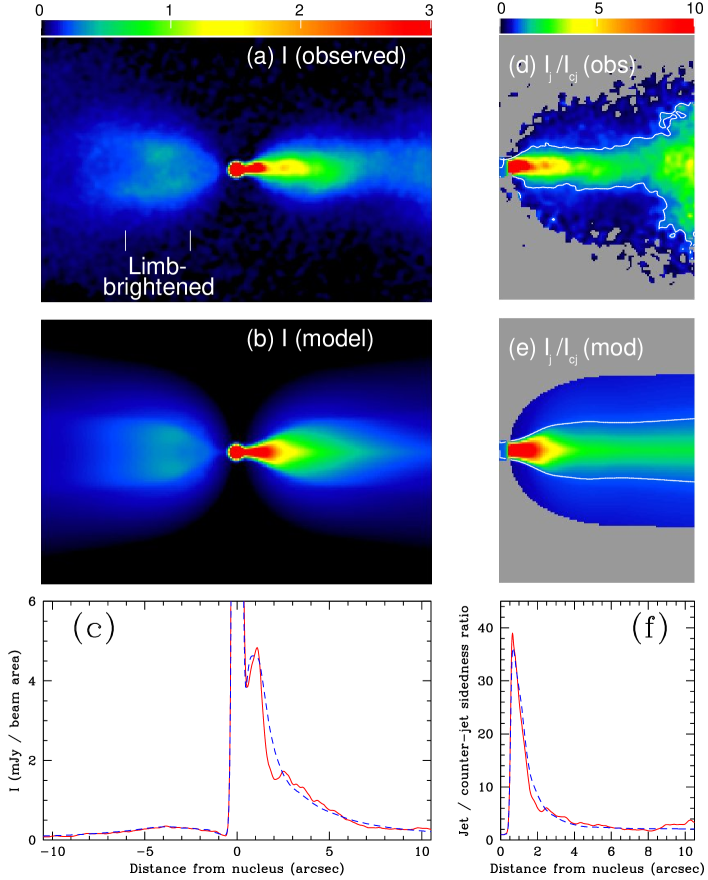
Figure 6: Comparison between the observed and modelled total intensities $I$ and sidedness ratios $I_{\rm j}/I_{\rm cj}$ for 0206+35. (a) observed and (b) model false-colour images of $I$. (c) profiles of observed (full/red) and model (dashed/blue) $I$ along the axis of the jet. (d) and (e) images of $I_{\rm j}/I_{\rm cj}$. The white contours represent $I_{\rm j}/I_{\rm cj}=1$: outside the contours, $I_{\rm j}/I_{\rm cj}<1$. (f) profiles of observed (full/red) and model (dashed/blue) $I_{\rm j}/I_{\rm cj}$ along the jet axis.

Figure 7: Comparison between the observed and modelled linear polarization of 0206+35. (a) and (b) colour images of degree of polarization $p=P/I$ in the range 0 – 0.7, as indicated by the labelled wedge. Blanked areas are grey. (a) observed; (b) model. (c) profiles of observed (full/red) and model (dashed/blue) $p$ along the axis of the jet. (d) and (e) vectors with lengths proportional to $p$ and directions along the apparent magnetic field superimposed on colour images of $I$. (d) observed, (e) model.

The quoted uncertainties were also derived as in our earlier work by varying an individual parameter until $\chi^{2}$ increased by an amount corresponding to the formal 99 per cent confidence level, leaving the rest of the model unchanged. These values are crude (they neglect coupling between parameters), but in practice give a good impression of the range of reasonable models. As an additional check, we also performed a series of optimizations at fixed values of $\theta$ and tabulate the range over which acceptable solutions could be found.

4 Model-data comparisons

4.1 General

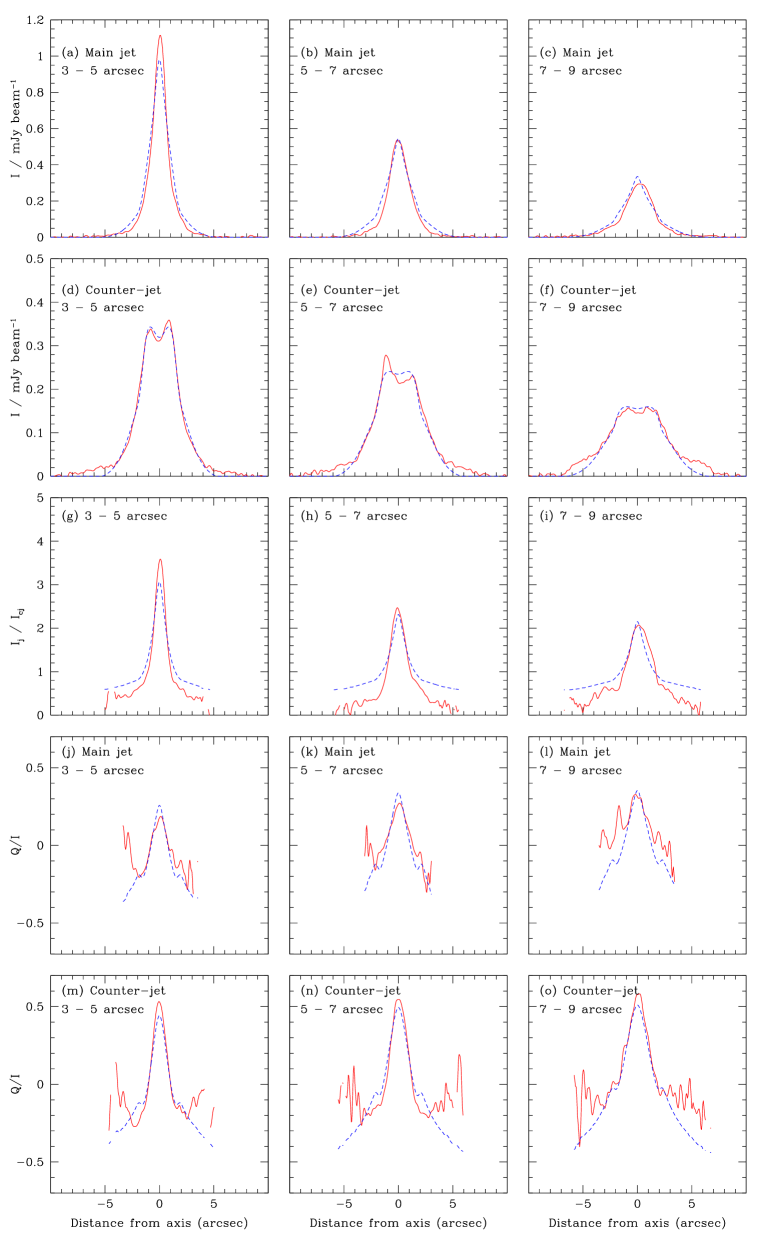
Figure 8: Transverse profiles of total intensity, $I$, jet/counter-jet sidedness ratio, $I_{\rm j}/I_{\rm cj}$ and $Q/I$ for 0206+35. The data have been averaged parallel to the jet axis over three ranges of distance from the nucleus: 3 – 5, 5 – 7 and 7 – 9 arcsec, as indicated in the captions (Section 4.1). Full/red line: observations; dashed/blue line: model. $Q/I>0$ and $Q/I<0$ correspond to transverse and longitudinal apparent field, respectively.

In Figs 6 – 8 and 10 – 12, we show various comparisons between the observed and model images of the two sources. The images have been rotated by the angles given in Table 2 so that the main (approaching) jet points to the right and the core is either at the centre or the left-hand edge of a plot. The types of plot are as follows.

1. False-colour images of total intensity. The angular scale is given on the accompanying profiles and the brightness range (in mJy beam^-1) is indicated by the labelled wedges.

2. Longitudinal profiles of total intensity.

3. Images of jet/counter-jet sidedness ratio $I_{\rm j}/I_{\rm cj}$ derived by dividing the $I$ image by a copy of itself rotated by 180^∘. These images are blanked (grey) where $I<3\sigma_{I}$ on either side of the core (Table 2). The contours show $I_{\rm j}/I_{\rm cj}=1$. Angular scales are again shown on the accompanying profiles.

4. Longitudinal profiles of sidedness ratio.

5. Images of degree of polarization, $p=P/I$. These are blanked wherever $I<5\sigma_{I}$. The angular scale is given on the accompanying profiles and the range is indicated by the labelled wedges. $p$ has been corrected for Ricean bias (Wardle & Kronberg, 1974).

6. Profiles of $p$ along the jet axis.

7. Vectors with lengths proportional to $p$ and directions along the apparent magnetic field, superposed on false-colour images of $I$. The angular and vector scales are indicated by labelled bars.

8. Averaged transverse profiles of total intensity, $I$, sidedness ratio $I_{\rm j}/I_{\rm cj}$, and $Q/I$ over selected regions where the brightness and polarization distributions vary slowly with distance from the nucleus. Stokes $Q$ is defined in a coordinate system with its axis along the jet: $Q/I>0$ for an apparent magnetic field transverse to the axis; $Q/I<0$ for a longitudinal field. In the flaring region, these profiles were derived by averaging along radii from the nucleus, in which case they are plotted against angle from the jet axis. For the outer region, they are averages along lines parallel to the jet axis and are plotted against angular distance from the axis. In order to make a fair comparison, only pixels which were not blanked on the observed images were used in the averages.

In general the fits are very good. We examine the correspondence between model and observed brightness distributions in detail in the next two sub-sections.

4.2 0206+35

We show images and longitudinal profiles of total intensity and sidedness ratio in Fig. 6 and of degree and direction of polarization in Fig. 7. Averaged transverse profiles of $I$, $I_{\rm j}/I_{\rm cj}$ and $Q/I$ are given in Fig. 8.

The model accurately reproduces the main features of the brightness and polarization distributions of 0206+35, including the following.

1. The main (approaching) jet has a bright base, with a peak at $\approx$2 arcsec from the nucleus (Figs 6a – c).

2. The peak sidedness ratio of $I_{\rm j}/I_{\rm cj}\approx 37$ is at a distance of $\approx$0.6 arcsec from the nucleus (Figs 6d – f), close to the position of the flaring point as determined from high-resolution MERLIN observations (Laing et al., 2011).

3. At low isophotes, the counter-jet appears wider than the main jet (Figs 6a and b).

4. The counter-jet has a limb-brightened structure, which is brightest between 2.5 and 6 arcsec from the nucleus, whereas the main jet appears narrower and is centrally peaked (Figs 6a and b; Figs 8a – f).

5. The longitudinal profile of degree of polarization shows the characteristic asymmetry we have noted in other FR I jets: the main jet has a polarization minimum at $\approx$2.5 arcsec from the nucleus, corresponding to the transition between longitudinal and transverse apparent field, whereas the counter-jet shows a high degree of polarization with a transverse apparent field, reaching an average of $p\approx 0.5$ at 10 arcsec (Fig. 7c).

6. There is a transition in the field direction between transverse on-axis and aligned with the jet boundaries at the edges on both sides of the nucleus. This is clear within 2 or 3 arcsec of the ridge line in the main and counter-jets, respectively (Fig. 7 and Figs 8j – o). The signal-to-noise ratio in the data is too low to determine the edge field direction accurately at larger distances, so discrepancies between observed and predicted $Q/I$ transverse profiles should not be taken too seriously.

7. Close to the nucleus, the apparent field wraps around the edges of both jets, with a high degree of polarization, especially on the counter-jet side (Figs 7d and e).

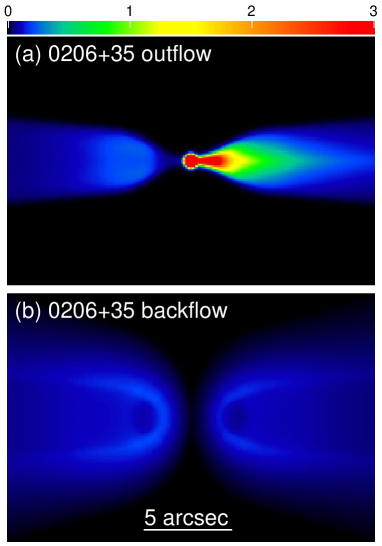
Figure 9: Predicted brightness distributions for the outflowing and backflowing parts of the model for 0206+35. (a) outflow; (b) backflow.

The main deficiency of the model is that it underpredicts the brightness of the counter-jet $\ga$5 arcsec from the axis and over-predicts that of the main jet between 1.5 and 4 arcsec. These effects lead to a model sidedness ratio which is too high off-axis, although still significantly $<$1. This discrepancy is most obvious between 5 and 7 arcsec from the nucleus (Figs 8b, e and h), but is restricted to regions where the brightness is $\la$200 $\mu$Jy beam^-1. The model is also constrained to have monotonic deceleration in the outflow and velocity independent of distance from the nucleus in the backflow, so it cannot reproduce the increase in sidedness ratio between 8 and 10 arcsec from the nucleus. The surface brightness is low at these distances so uncertainties in lobe subtraction may be significant.

Fig. 9 shows the predicted brightness distributions for the outflowing and backflowing parts of the model separately. The former is similar to the pure outflow models we have derived for other sources (Laing & Bridle, 2002a; Canvin & Laing, 2004; Canvin et al., 2005; Laing et al., 2006a). In the model of 0206+35, the limb-brightening of the counter-jet is due to a combination of outflow and backflow. In the outflow, the on-axis velocity remains high, so the edges of the outflowing counter-jet material appear relatively brighter because they suffer less Doppler dimming than the on-axis material. This effect is reinforced by emission from the backflow, which adds a thin shell of emission immediately surrounding the outflow. Most of the asymmetry is due to the outflow: the backflow is only slightly brighter on the counter-jet side.

4.3 0755+37

We compare model and observed total intensity images and profiles for 0755+37 in Fig. 10; the corresponding polarization comparisons are shown in Fig. 11 and Fig. 12 gives averaged transverse profiles of $I$, $I_{\rm j}/I_{\rm cj}$ and $Q/I$. Note that the fainter emission is affected by imperfect lobe subtraction, as discussed in Section 2.2. This is particularly obvious at large distances from the jet axis in images of ratios such as $I_{\rm j}/I_{\rm cj}$ and $p$. The following features of the brightness and polarization distributions are reproduced.

1. The main jet has a brightness peak at 1.3 arcsec from the core (Figs 10i – k). Farther out, the profile declines rapidly with distance.

2. There is a rapidly-expanding, triangular region of roughly uniform brightness at the base of the counter-jet (Figs 10a and b).

3. The jet base structure is initially very asymmetric, with a peak sidedness ratio $\approx$80 at 1.9 arcsec from the core, decreasing rapidly with distance to reach an asymptotic value $\approx$1 at 15 arcsec (Figs 10e – h).

4. At faint brightness levels, the counter-jet appears significantly wider than the main jet, with a large opening angle (Figs 10a and b).

5. The counter-jet brightness profiles are more flat-topped or edge-brightened than those of the main jet at most distances from the core (Figs 10a and b and Figs 12a – h).

6. A prominent arc of emission crosses the counter-jet at $\approx$26 arcsec from the nucleus (Figs 10a and b).

7. There is also a bar of emission crossing the counter-jet at $\approx$12 arcsec from the nucleus (Figs 10a, b and d).

8. The profiles of degree and direction of polarization along the axis show the same characteristic asymmetry seen in 0206+35 and other FR I jets. There is a change in apparent field direction at $\approx$5 arcsec from the nucleus in the approaching jet, but not in the counter-jet, whose apparent magnetic field is always transverse (Figs 11g and h, Figs 12q – t). The degree of polarization in the counter-jet rises monotonically with distance from the nucleus, reaching large values ($p\approx 0.5$) far from the nucleus (Figs 11a – c).

9. The degree of polarization in the main jet base is low, and the apparent field is longitudinal (Figs 11d – f, i and j).

10. There are minima in the degree of polarization on either side of the axis in both jets, corresponding to the transition between transverse and longitudinal apparent field (Figs 11a, b, g, h; 12m – t).

11. There is a region of high polarization with a circumferential magnetic field around the base of the counter-jet (Figs 11g and h).

12. Determination of the observed polarization in the faint regions far from the axis is complicated by imperfect subtraction of lobe emission, but the apparent field is primarily parallel to the edges of both jets (Figs 12m – t).

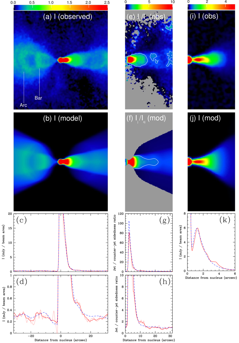
Figure 10: Comparison between the observed and modelled total intensities $I$ and sidedness ratios $I_{\rm j}/I_{\rm cj}$ for 0755+37. (a) and (b) colour images of $I$. (a) observed; (b) model. (c) and (d) profiles of observed and model $I$ along the axis of the jet. (e) and (f) images of $I_{\rm j}/I_{\rm cj}$. The white contours represent $I_{\rm j}/I_{\rm cj}=1$: outside the contours, $I_{\rm j}/I_{\rm cj}<1$. (g) and (h) profiles of observed and model $I_{\rm j}/I_{\rm cj}$ along the jet axis. The resolution for panels (a) – (h) is 1.3 arcsec FWHM. (i) and (j) colour images of $I$ in the range 0 – 5 mJy beam^-1 for the base of the main jet. (i) observed, (j) model. (k) profile of observed and model $I$ along the jet axis. The resolution for panels (i) – (k) is 0.4 arcsec FWHM. In the profile plots, the full and dotted (red) lines are from observed images with lobe subtraction by interpolation (as for the colour plots) and spectrum, respectively. The dashed/blue line is the model.

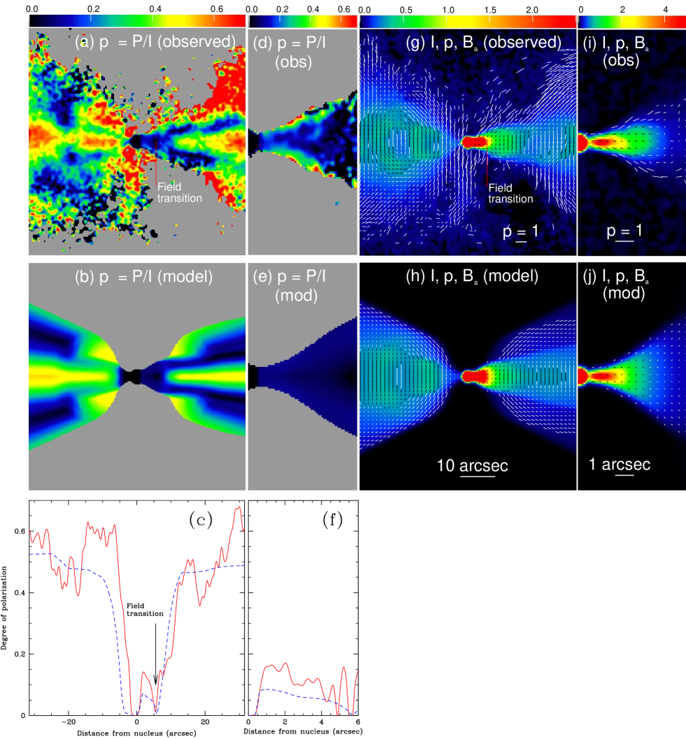
Figure 11: Comparison between the observed and modelled linear polarization for 0755+37 at resolutions of 1.3 and 0.4 arcsec FWHM. (a) and (b) colour images of $p=P/I$ in the range 0 – 0.7 at 1.3 arcsec FWHM. (a) observed; (b) model. (c) profiles of observed (full/red) and model (dashed/blue) $p$ along the axis of the jet. Only the profile of $p$ derived from interpolated images is plotted; the equivalent for spectral subtraction is very noisy. (d) – (f): as (a) – (c) but for the main jet only at 0.4 arcsec FWHM. (g) and (h): vectors with lengths proportional to $p$ and directions along the apparent magnetic field superimposed on colour images of $I$. The resolution is 1.3 arcsec FWHM and the vector scale is indicated by the labelled bar. (g) observed, (h) model. (i) and (j): as (g) and (h), but for the main jet at 0.4 arcsec FWHM.

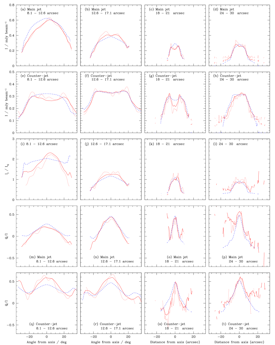
Figure 12: Transverse profiles of total intensity, $I$, jet/counter-jet sidedness ratio, $I_{\rm j}/I_{\rm cj}$ and $Q/I$ for 0755+37. The data have been averaged along radii from the nucleus from 8.1 – 12.6 arcsec and from 12.6 – 17.1 arcsec and parallel to the jet axis from 18 – 21 arcsec and 24 – 30 arcsec, as indicated in the captions (Section 4.1). Full and dotted (red) lines both represent observations, with lobe subtraction by interpolation and spectral methods, respectively. Dashed/blue lines show the model. $Q/I>0$ and $Q/I<0$ correspond to transverse and longitudinal apparent field, respectively.

Features which are not fit well by the model are as follows.

1. The observed brightness distribution of the bright main jet base is slightly more centre-brightened than the model and the observed degree of polarization is higher than predicted at its edges (Figs 10i, j; 11d, e, i, j).

2. The observed transverse total-intensity profiles are significantly more limb-brightened than the model in some places, and in particular between 18 and 21 arcsec on both sides of the nucleus (Figs 12c and g).

3. The inner bar crossing the counter-jet is both straighter and slightly farther from the nucleus in the observed image ($\approx$13 arcsec compared with $\approx$11 arcsec for the model; Figs 10a, b, d). The fit may be affected by the limb-brightening in this region, however.

4. As in 0206+35, the off-axis brightness of the main jet is slightly overestimated close to the nucleus. The difference is, however, exaggerated by the look-up table in Figs 10(a) and (b) and is more accurately represented by the profile in Fig. 12(a).

Fig. 13 shows the outflow and backflow components of the model intensity distribution. As for 0206+35, the outflow appears similar to that in other FR I radio galaxies, but the backflow is relatively stronger in 0755+37. The prominent curved arc crossing the counter-jet $\approx$26 arcsec from the nucleus is modelled as the projection of the inner edge of the backflow at $r=r_{\rm b}$. This is roughly elliptical in shape, with an axial ratio of $\sec\theta=1.22$ and there is good correspondence between model and data. As mentioned earlier, the fit to the bar crossing the counter-jet closer to the nucleus is less successful. In the model, this is the other half of the projected inner edge of the backflow, so there is no freedom to adjust its location or curvature to match the observed feature more closely. A similar problem afflicts the main jet: the projection of the inner edge of the backflow appears slightly too bright, causing the excess off-axis emission close to the nucleus.

5 Derived parameters

The best-fitting parameters for our models of 0206+35 and 0755+37 are listed in Tables 5 (outflow) and 6 (backflow).

5.1 Geometry

Both sources are fairly close to the line of sight, as expected from their high jet/counter-jet sidedness ratios and bright cores. We derive $\theta=40^{\circ}$ for 0206+35 and $35^{\circ}$ for 0755+37. The outflow geometries are typical of those we have determined for other FR I jets, with the boundaries between flaring and outer regions at 5.3 and 13.9 kpc from the nucleus for 0206+35 and 0755+37, respectively. The corresponding half-opening angles in the outer regions are 3$\aas@@fstack{\circ}$9 and 7$\aas@@fstack{\circ}$4.

In 0206+35, the backflow has a half-opening angle of 11° in the outer region and its emission extends back into the flaring region, with a cut-off at $r_{\rm b}=2.7$ kpc. For 0755+37, on the other hand, the backflow emission is truncated within the outer region ($r_{\rm b}=23$ kpc), where its half-opening angle is 16°.

5.2 Velocity

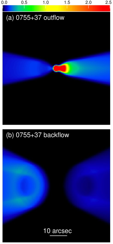
Figure 13: Predicted brightness distributions for the outflowing and backflowing parts of the model for 0755+37. (a) outflow; (b) backflow.

Velocity images derived from our model fits are shown in Fig. 14.

The initial velocities of both outflow components are similar ($\beta_{1}=0.86$ for 0206+35 and 0.88 for 0755+37) and the associated transverse velocity profiles are close to uniform. 0206+35 shows little on-axis deceleration, reaching an asymptotic velocity $\beta_{0}=0.68$ after 4 kpc. Its transverse velocity profile evolves much more, and the fractional edge velocity is 0.04 at large distances. In both these respects, the source resembles 3C 296 (Laing et al., 2006a). 0755+37, on the other hand, appears to decelerate rapidly, to $\beta_{0}=0.25$ by 18.5 kpc, with a fractional edge velocity of 0.26. This estimate should be treated with caution since the emission in the outer counter-jet is dominated by the backflow component, making it difficult to assess the intensity or polarization of the outflow there.

The backflow velocities increase away from the source axis, from $\beta=0.05$ to 0.20 for 0206+35 and from 0.25 to 0.35 for 0755+37.

5.3 Emissivity

Model images of $n_{0}B^{1+\alpha}$ (proportional to the emissivity function $\epsilon$) are shown in Fig. 15.

The model outflow components again show properties very similar to those in other FR I jets. The locations of the flaring points (0.82 and 1.55 kpc from the nucleus for 0206+35 and 0755+37, respectively) are well determined and consistent with higher-resolution observations (Laing et al., 2011). The emissivity variations in the faint and poorly resolved inner jets upstream of the flaring points are not well constrained. In the flaring and outer regions, the gradient of the emissivity profile flattens with distance in both sources, as is usual in FR I jets. 0755+37 requires a sudden decrease in emissivity with distance at $r=r_{e0}$ whereas 0206+35 does not.

The observed limb-brightening in both sources shows side-to-side symmetry. This cannot result from a transverse velocity gradient in the sense we have inferred, which would lead to limb-brightening only in the counter-jet. In agreement with this qualitative argument, the best-fitting transverse emissivity profiles are higher at the edges than on-axis. This effect is slight in 0206+35, where the profile is consistent with a uniformly-filled cylinder everywhere. In 0755+37, however, limb-brightening is required over much of the outer region (Fig. 15b). As noted in Section 4.3, the observed transverse intensity profiles in this source are significantly more limb-brightened than the model predicts, suggesting that there is a narrow enhancement in emissivity at the boundary between the outflow and backflow. The functional form we assume for the transverse variation of emissivity does not allow for such narrow features.

The backflow emissivity decreases with distance at similar rates in the two sources ($\propto r^{-1.66}$ in 0206+35 and $\propto r^{-1.81}$ in 0755+37). It is centre-brightened in 0206+35 ($e_{\rm b}=0.02$) but closer to uniform in 0755+37 ($e_{\rm b}=0.79$).

5.4 Field Ordering

The fractional components of magnetic field, $\langle B^{2}_{t}\rangle^{1/2}/B$ (toroidal), $\langle B^{2}_{l}\rangle^{1/2}/B$ (longitudinal), and $\langle B^{2}_{r}\rangle^{1/2}/B$ (radial) are plotted in Fig. 16.

In both sources, the field close to the nucleus in the outflow is close to isotropic, with the longitudinal component just exceeding the other two. At larger distances, the toroidal component dominates, with significant longitudinal and radial contributions in 0206+35 and 0755+37, respectively. As for velocity and emissivity, the field components in the outer parts of 0755+37 may have larger systematic errors because of the dominance of backflow emission.

The field in the backflow is toroidally dominated in both sources, with non-negligible radial components in both cases and some longitudinal field in 0206+35.

Table 5: Model parameters which are common to outflow and backflow, or which apply only to the outflow (Section 3.3 and Table 4). Col. 1: parameter; col. 2: unit; cols 3 and 4: values for 0206+35 and 0755+37. The parameters are defined in Section 3.3 and listed in Table 4. $\Delta\theta$ is the range of angles to the line of sight for which any acceptable solutions can be obtained.

Variable		0206+35	0755+37
Geometry (common to outflow and backflow)
$\theta$	deg	$40.0_{-0.3}^{+0.3}$	$34.8_{-0.8}^{+0.7}$
$\Delta\theta$	deg	$34-43$	$32.5-37.5$
$r_{0}$	kpc	$5.3_{-0.1}^{+0.1}$	$13.9_{-0.3}^{+0.3}$
Outflow geometry
$\xi_{0}$	deg	$3.9_{-0.2}^{+0.2}$	$7.4_{-0.1}^{+0.2}$
$x_{0}$	kpc	$1.32_{-0.04}^{+0.02}$	$3.88_{-0.06}^{+0.08}$
Velocity
$r_{v1}$	kpc	$1.8_{-0.3}^{+0.3}$	$3.6_{-1.5}^{+1.6}$
$r_{v0}$	kpc	$4.1_{-0.2}^{+0.3}$	$18.5_{-1.5}^{+2.3}$
$\beta_{1}$		$0.86_{-0.07}^{+0.08}$	$0.88_{-0.04}^{+0.05}$
$\beta_{0}$		$0.68_{-0.05}^{+0.09}$	$0.25_{-0.05}^{+0.07}$
$v_{1}$		$0.95_{-0.13}^{+0.05}$	$1.00_{-0.06}$
$v_{0}$		$0.04_{-0.01}^{+0.02}$	$0.26_{-0.11}^{+0.19}$
Emissivity
$r_{e1}$	kpc	$0.82_{-0.02}^{+0.02}$	$1.55_{-0.03}^{+0.04}$
$r_{e0}$	kpc	$2.04_{-0.06}^{+0.07}$	$10.2_{-0.3}^{+0.1}$
$E_{\rm in}$		$\approx 3.1$	$\approx 2.4$
$E_{\rm mid}$		$2.59_{-0.08}^{+0.09}$	$3.76_{-0.04}^{+0.02}$
$E_{\rm out}$		$2.13_{-0.06}^{+0.08}$	$1.16_{-0.09}^{+0.05}$
$e_{1}$		$1.2_{-0.5}^{+0.6}$	$1.0_{-0.2}^{+0.3}$
$e_{0}$		$1.14_{-0.16}^{+0.16}$	$2.2_{-0.3}^{+0.5}$
$g_{1}$		$1.7_{-1.3}^{+0.8}$	$1.7_{-0.4}^{+0.5}$
$g_{0}$		$1.05_{-0.09}^{+0.08}$	$0.52_{-0.03}^{+0.06}$
Field component ratios
$r_{B1}$	kpc	$<1.4$	$8.8_{-2.0}^{+2.8}$
$r_{B0}$	kpc	$4.6_{-0.5}^{+0.5}$	$15.4_{-3.2}^{+2.5}$
$j_{1}$		$1.50_{-0.22}^{+0.34}$	$0.96_{-0.09}^{+0.13}$
$j_{0}$		$0.11_{-0.11}^{+0.13}$	$0.44_{-0.15}^{+0.12}$
$k_{1}$		$1.36_{-0.13}^{+0.13}$	$1.15_{-0.07}^{+0.08}$
$k_{0}$		$0.64_{-0.04}^{+0.05}$	$0.08_{-0.08}^{+0.22}$

Table 6: Model parameters for backflow (Section 3.3 and Table 4). Col. 1: parameter; col. 2: unit; cols 3 and 4: values for 0206+35 and 0755+37.

Variable		0206+35	0755+37
Geometry
$\xi_{\rm b}$	deg	$10.9_{-0.5}^{+0.5}$	$15.6_{-0.1}^{+0.5}$
$r_{\rm b}$	kpc	$2.7_{-0.2}^{+0.1}$	$23.2_{-0.7}^{+0.8}$
Velocity
$\beta_{\rm b,in}$		$0.02_{-0.02}^{+0.03}$	$0.25_{-0.07}^{+0.04}$
$\beta_{\rm b,out}$		$0.20_{-0.07}^{+0.06}$	$0.35_{-0.05}^{+0.05}$
Emissivity
$n_{\rm b}$	$\times 100$	$2.3_{-0.2}^{+0.2}$	$0.094_{-0.010}^{+0.000}$
$E_{\rm b}$		$1.66_{-0.07}^{+0.06}$	$1.81_{-0.05}^{+0.07}$
$e_{\rm b}$		$0.05_{-0.01}^{+0.02}$	$0.79_{-0.14}^{+0.13}$
Field component ratios
$j_{\rm b}$		$0.24_{-0.07}^{+0.08}$	$0.38_{-0.07}^{+0.07}$
$k_{\rm b}$		$0.38_{-0.09}^{+0.08}$	$0.03_{-0.03}^{+0.15}$

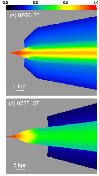
Figure 14: The model values of velocity $\beta$ in units of $c$ in planes containing the jet axes. Positive and negative values of $\beta$ denote outflow and backflow, respectively. (a) 0206+35, (b) 0755+37.

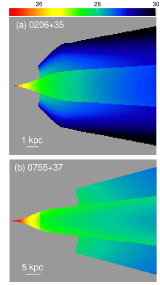
Figure 15: The model values of $\log(n_{0}B^{1+\alpha})$ in planes containing the jet axes ($n_{0}$ and $B$ are in SI units). (a) 0206+35, (b) 0755+37.

5.5 Backflow spectral index

We can also constrain the spectral index of the radio emission from the backflows. The spectral indices at the edges of the jets, where the line of sight is mainly through backflow emission after the lobe subtraction, are much closer to those of the jets themselves than to the values elsewhere in the lobes. We can estimate the spectrum of the backflow emission directly from the images shown in Figures 3(c) and 4(c) or, more accurately, by integrating total intensity at 1.425 and 4.860 GHz over pixels which are unblanked in these images. The latter method gives mean spectral indices of 0.50 for 0206+35 and 0.57 for 0755+37, compared with 0.55 and 0.53 for the sum of outflow and backflow emission.

6 Discussion

6.1 Testing the hypothesis

It is clear that the initial jet base asymmetries of most FR I jets are produced by relativistic aberration (Laing & Bridle, 2002a; Canvin & Laing, 2004; Canvin et al., 2005; Laing et al., 2006a). If 0206+35 and 0755+37 prove to be typical – in that counter-jets consistently appear wider than the main jets at a given isophote in lobed FR I sources whose jet base asymmetries are large – then the jet/counter-jet width asymmetry must also be correlated with jet orientation. The models presented in Section 4 show that mildly relativistic backflow offers a possible cause for such an orientation-dependent effect.

There is an alternative explanation for $I_{\rm j}/I_{\rm cj}$ becoming $<$1 in some parts of a source which also preserves the orientation-dependence of the effect. For the special case where the magnetic field is purely toroidal and the edge velocity is $\approx\cos\theta$, it is possible for relativistic aberration to give an off-axis jet/counter-jet sidedness ratio $<$1 even for a pure symmetrical outflow. We analyse this special case in Appendix A, where we show that it is inconsistent with the polarization imaging of 0206+35 and 0755+37. The mechanism inevitably produces degrees of polarization close to the theoretical maximum of $p_{0}\approx 0.7$ with a transverse apparent field. It is therefore unlikely to be important in the majority of observed jets but it may be relevant in a few objects like 3C 296 (Appendix A).

If the jets are intrinsically symmetrical, then the backflow hypothesis remains the most plausible explanation for the observed brightness and polarization asymmetries, but (with only two clear-cut cases analysed in such detail so far) it is important to test it by looking at more objects. We reviewed the rest of the B2 low-luminosity source sample (Parma et al., 1987) to see if any other data support (or contest) the interpretation given here. Laing et al. (1999) found that the source B2 0844+31 also has both a small jet to counter-jet width ratio and a high intensity ratio $I_{\rm j}/I_{\rm cj}$. Unfortunately, there is no imaging for that source of the high quality we now have for 0206+35 and 0755+37 so we cannot test models of its asymmetries at the same level of detail. Nor can we classify its large scale structure definitively as ‘lobed’ or ‘plumed’: deeper imaging sensitive to its most extended structure is needed. Although lack of high-quality imaging precludes us from finding other good examples of these phenomena in the B2 sample, we note that there are no clear counter-examples – either of sources in which the brighter jet appears to be wider than the counter-jet at low intensity levels, or of a large jet/counter-jet width asymmetry in a source that lacks ‘lobed’ structure or with only a small jet/counter-jet intensity asymmetry at its base.

As noted by Laing et al. (2006a, see their fig. 15), the jets in the lobed FR I source 3C 296 show $I_{\rm j}/I_{\rm cj}<1$ at their edges. The emission there is faint, but the effect is consistently present in the flaring and outer regions. The transverse variations of linear polarization are also very different in the two jets (Laing et al., 2006a, Figs 18g and h): the counter-jet shows a prominent parallel-field edge, whereas the main jet does not. The model described by Laing et al. (2006a), while giving a good overall fit to the brightness and polarization distributions of 3C 296, was not consistent with the observation of $I_{\rm j}/I_{\rm cj}<1$ and did not fully reproduce the flat profile of $p$ with transverse apparent field in the approaching jet. We have examined possible backflow models for 3C 296 and find that they are qualitatively inconsistent with the polarization distribution, although they can easily fit the edge sidedness ratios. The combination of sidedness ratio and polarization is more reminiscent of the predictions of the outflow model analysed in Appendix A.

Emission from backflow such as that modelled here would be hard to recognise in lobed FR I sources whose jets are close to the plane of the sky. The backflow emission in such sources would be almost indistinguishable from faint outer edges of their jets and only unusually precise spectral index measurements could distinguish it from low level brightness enhancements of the lobes near the jets.

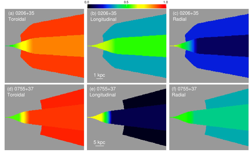
Figure 16: The fractional magnetic field components for the three sources. (a), (d) toroidal, $\langle B_{t}^{2}/B^{2}\rangle^{1/2}$; (b), (e) longitudinal, $\langle B_{l}^{2}/B^{2}\rangle^{1/2}$; (c), (f) radial, $\langle B_{r}^{2}/B^{2}\rangle^{1/2}$. (a) – (c) 0206+35, (d) – (f) 0755+37.

6.2 Should we expect backflows in FR I sources?

Light jets propagating into dense media can be expected to terminate in one of two ways. They may decelerate and transition into ‘plumes’ or ‘tails’ that are deflected away from the AGN by external pressure gradients or by winds in the IGM. Alternatively, they may deflect before reaching a contact discontinuity with the denser external medium, thus accumulating a ‘cocoon’ around the outflow. The first process is thought to underlie the formation of plumed or tailed FR I radio sources such as 3C 31 while the second is thought to form the ‘classical double’ lobed radio sources such as Cygnus A and is often associated with FR II morphology. Lobes in the (generally more luminous) FR II sources also frequently contain discrete radio ‘hot spots’ that are identified with strong shocks where well-collimated (supersonic) outflows are slowed and begin to supply lobe material. There is no reason to suppose, however, that discrete hot spot formation is a requisite for cocoon (or radio lobe) formation – momentum balance alone requires the deflection of the light outflow if it cannot escape along its initial path owing to development of a high pressure region downstream. Cocoons without hot spots are indeed seen in simulations of relativistic jets which are much lighter than their surroundings (Perucho & Martí, 2007; Rossi et al., 2008), in which the jets flows are transonic where they terminate.

The majority of FR I sources form radio lobes whose detailed morphologies, spectral characteristics and polarization properties strongly resemble those of higher-power FR II lobes (Parma et al., 1996, 1999; Laing et al., 2011). Their lobes have sharp outer brightness gradients, circumferential magnetic fields, and spectral indices that steepen towards the centre of the source on the largest angular scales – but without hot spots. Furthermore, outflows in lobed FR I sources can deflect through large angles without losing their identities: Laing et al. (2011) found regions where emission with jet-like spectral index $\approx$0.6 had displaced steeper-spectrum emission within FR I lobes. These results suggest that ongoing large-scale flow is present in these lobes well beyond the clearly recognisable jets.

There is therefore both theoretical and observational support for supposing that jet outflows containing relativistic particles and magnetic fields may be redirected through large angles in lobed FR I sources. The additional ingredient suggested by our modelling of 0206+35 and 0755+37 is that a component of such an outflow in an FR I source can return to the vicinity of the AGN as mildly relativistic backflow. As we noted in the introduction to this paper, this idea is supported by the presence of backflow with $\beta\ga 0.2$ around the jets in some numerical simulations of the propagation of light, relativistic jets. The simulation by Perucho & Martí (2007) used initial conditions for the jet derived from our FR I source models (Laing & Bridle, 2002a, b) and realistic density and pressure gradients in the surrounding galactic and group atmosphere (Hardcastle et al., 2002). In particular, the velocity at injection was $\beta=0.87$ and the initial density contrast (the ratio of the density of the jet to that of its surroundings) was $\eta=10^{-5}$. Although the jet had propagated only $\approx$15 kpc by the end of the simulation, the structure already resembled a lobed FR I source of the type discussed here, with a cocoon of backflowing, mixed jet and external plasma surrounding the jet. The jet was transonic at its termination, so no hot spot was formed. Typical backflow velocities in the cocoon were $\beta\approx 0.15$, with values reaching $\beta\approx 0.4$ close to the nucleus. The use of an open boundary condition in the symmetry plane at the base of the jet can cause the backflow speed to be over-estimated (Saxton et al., 2002), although Perucho & Martí (2007) argued that this effect was small in their simulation because the flow through the open boundary was negligible. One other possible concern is that the simulation by Perucho & Martí (2007) was axisymmetric: the speed and extent of fast backflow appear to be smaller in some fully three-dimensional simulations compared with the equivalent axisymmetric cases (Norman, 1996; Aloy et al., 1999). We note, however, that the comparison may not be relevant to lobed FR I sources because the density contrast, $\eta=0.01$, was much higher in these two examples, leading to cocoons which were far longer and thinner than those observed. The three-dimensional simulation of a relativistic jet with $\eta=10^{-4}$ by Rossi et al. (2008) indeed showed fast backflow with $\beta\approx 0.4$, despite the use of symmetric boundary conditions at the jet inlet. The initial conditions (jet Lorentz factor $\Gamma=10$) and the assumption of a uniform external density are probably more appropriate to smaller physical scales than we consider here, however. Thus, although the assumptions and initial conditions of the simulations by Perucho & Martí (2007) and Rossi et al. (2008) are not realistic enough to permit a quantitative comparison with our results, they do suggest that the idea of fast backflow is a reasonable one provided that the density contrast is very small ($\la 10^{-4}$).

The simulations discussed above are entirely hydrodynamic. We also note that backflow is an expected ingredient of models of magnetic hoop stress collimation of current-carrying jets because such models must provide a return current path – although it is unclear that such return paths need be as close to the jet outflow boundary as the backflow we have described here.

7 Summary and Further Work

7.1 Summary

We have shown that many aspects of the intensity and linear polarization distributions over the inner jets and counter-jets in the lobed FR I radio sources 0206+35 and 0755+37 are accounted for by an intrinsically symmetrical decelerating relativistic jet model that includes (mildly) relativistic backflow around both jets.

We have estimated properties of this backflow subject to the simplifying assumptions that it is symmetrical across the AGN, axisymmetric, and that its streamlines are similar in shape to those of the outflow. Although these assumptions are likely to be too simple a priori we nevertheless find that the quality of the $IQU$ fits obtained with the models including such symmetric backflow is similar to that obtained with pure decelerating outflow models of other FR I jets (Laing & Bridle, 2002a; Canvin & Laing, 2004; Canvin et al., 2005; Laing et al., 2006a). Furthermore, the outflow components of the models we have fitted to 0206+35 and 0755+37 are quite similar to those obtained for other FR I sources. The addition of backflow to the models therefore suffices to explain the otherwise anomalous jet/counter-jet asymmetries of both sources and eliminates the need to invoke ad hoc environmental (or other intrinsic) side-to-side asymmetries.

The salient features of backflow inferred from this procedure are as follows.

1. The backflow velocities are mildly relativistic, in the range $0.05\la\beta\la 0.35$ (Fig. 14).

2. The backflows are approximately symmetric around the outflows and their radio emission comes from a hollow cone surrounding the jet axis with additional half-opening angles $\approx 8\degr$.

3. They can be traced to considerable distances from the AGN (at least 15 kpc for 0206+35 and 50 kpc for 0755+37) but the emission close to the ends of the jets in both sources is chaotic, and it is not clear where the backflows begin.

4. They do not emit synchrotron radiation all the way in to the AGN (Fig. 15).

5. The backflows emit with a spectral index $\alpha\approx 0.55$ (Section 5.5). This spectral index is lower than that of the nearby lobes and comparable with those of the outflows.

6. Their magnetic fields are mostly toroidal and their emissivities decrease with distance roughly as $r^{-1.7}$ (Figs 15 and 16).

These are the only two lobed FR I sources for which we have deep enough imaging and polarimetry to reveal the ‘two-component’ aspect of the jets and counter-jets that motivated this study. The generality of our results could thus be called into question by a single new example of an FR I source with strong jet-width asymmetries in which either (a) the axis is inferred to be close to the plane of the sky or (b) the apparently wider features are associated with the brighter jet. With only two examples of possible backflow features we also cannot address whether all lobed FR I sources might contain backflow or (conversely) whether backflow exists only in lobed sources.

The interpretation including backflow will continue to be preferable to any involving intrinsic side-to-side width differences if further studies find the apparently wider features only on the counter-jet side, and only in lobed sources for which inclination indicators suggest that the jets are at moderately large angles to the plane of the sky.

7.2 Open questions and further work

Our observations and models give no clue about the ultimate fate of the backflow or how it may interact with the outflow, but they raise a number of questions which could be addressed by deeper, higher-resolution observations of 0206+35 and 0755+37.

1. Where does the backflow originate? Does it start in a high-pressure region at the end of the outflow?

2. Does the backflow shield the jet from entrainment or interaction with the lobe plasma?

3. Does the presence of the backflow perturb the jet structure in any way?

4. Where does the backflow ultimately go: sideways or even closer to the AGN?

5. Why does the backflow radiate strongly where it does and stop radiating close to the AGN?

6. Can the backflow really be faster than the asymptotic velocity of the outflow, as appears at first sight to be the case in 0755+37?

Additional questions which could be answered by observations of a sample of FR I sources include the following.

1. Do jets in other FR I sources with large jet-width asymmetries also have the two-component jet and counter-jet structure found here in 0206+35 and 0755+37 (i.e. a strongly centrally brightened peaked main jet and centre-darkened counter-jet near the axis, and counter-jet emission consistently brighter than that of the main jet further from the axis)?

2. Does the counter-jet/jet width asymmetry indeed correlate well with orientation indicators – counter-jet/jet intensity ratios and normalized core power – as expected in a relativistic backflow model of this asymmetry? If so, the tightness of the correlation with orientation indicators could be used to constrain the intrinsic symmetry of the backflow.

3. Does the width asymmetry indeed occur only in lobed FR I’s? It will be important to obtain images which are sufficiently sensitive to extended structure to detect faint lobe emission in any sources whose structural classification is dubious.

The high sensitivity and resolution of the imaging needed to address all of these issues and to test backflow models of the type we have proposed will require the use of the Jansky (Expanded) Very Large Array and e-MERLIN.

Given the similarities between the extended emission in FR II and lobed FR I sources, it would also be interesting to search for evidence of backflow in the former class. The jets in FR II sources are usually much narrower than those we have imaged in the present study and are thought to be highly supersonic where they terminate in compact hot spots. Backflow is predicted by simulations of FR II dynamics, but it is unclear how its properties might depend on density contrast, Mach number, magnetization and source age. It may be that observations of FR II sources without prominent hot spots will offer the best chance of detecting backflows. Counter-jets in FR II sources are faint and difficult to distinguish from filamentary lobe emission, so identification of any backflow component may be even more challenging than in FR I’s.

Three-dimensional simulations of very light, relativistic jets propagating in realistic external density and pressure distributions would be extremely valuable in understanding the backflow phenomenon in FR I sources. To be realistic, such simulations should be bipolar, with initial density contrasts $\approx$10^-5. The effects of magnetic fields (ordered or disordered) on the flow also remain to be investigated.

Appendix A Pure outflow models with $I_{\rm j}/I_{\rm cj}<1$

It is possible under some circumstances for the ratio $I_{\rm j}/I_{\rm cj}$ (approaching/receding) to be significantly less than unity close to the edges of the brightness distribution even for a symmetrical outflow. This might easily be mistaken for the effects of a backflowing component. We argue in this Appendix that the effect is quite likely to be observed in FR I jets, but that it is qualitatively inconsistent with the observations of 0206+35 and 0755+37 (particularly in linear polarization). 3C 296 (modelled as a pure outflow by Laing et al. 2006a) may show this effect at low brightness levels.

$I_{\rm j}/I_{\rm cj}$ can become $<1$ because of the effect of aberration on anisotropic rest-frame emission. If this acts in such a way that the magnetic field is nearly parallel to the line of sight in the rest frame, then the synchrotron emissivity can become very low. If this happens in the approaching jet but not the receding one, then the effect may be larger than that of Doppler boosting. A symmetrical pair of jets with purely toroidal fields can show this effect for some ranges of velocity. If the condition $\beta=\cos\theta$ is satisfied at the edge of the approaching jet, then the field will be exactly parallel to the line of sight in the rest frame, so the synchrotron emissivity will be exactly zero. The condition can never be satisfied in the receding jet (except in the trivial case of a side-on source with zero velocity), so the sidedness ratio is also zero. Close to the jet edge or if the velocity condition is approximately satisfied, the sideness ratio can still be significantly less than unity.

In order to demonstrate the effect, we consider a simple model with symmetrical, cylindrical, constant-velocity jets containing purely toroidal fields. We also take the magnetic field and radiating particle density to be constant and assume $\alpha=1$ so that the calculated emission profiles are analytical, as given in the non-relativistic case by Laing (1981). Suppose that $x$ is a coordinate in the plane of the sky perpendicular to the projected jet axis and normalized by the jet radius. Then the transverse profiles of sidedness and $Q/I$ are given by:

$$\frac{I_{\rm j}(x)}{I_{\rm cj}(x)}=\left(\frac{D_{\rm j}}{D_{\rm cj}}\right)^{3}\frac{(1-x^{2})^{1/2}-D_{\rm j}^{2}\sin^{2}\theta|x|\arccos|x|}{(1-x^{2})^{1/2}-D_{\rm cj}^{2}\sin^{2}\theta|x|\arccos|x|}$$ (1)

$$\frac{Q_{\rm j}(x)}{I_{\rm j}(x)}=\frac{3}{4}\frac{(1-x^{2})^{1/2}-(2-D_{\rm j}^{2}\sin^{2}\theta)|x|\arccos|x|}{(1-x^{2})^{1/2}-D_{\rm j}^{2}\sin^{2}\theta|x|\arccos|x|}$$ (2)

$$\frac{Q_{\rm cj}(x)}{I_{\rm cj}(x)}=\frac{3}{4}\frac{(1-x^{2})^{1/2}-(2-D_{\rm cj}^{2}\sin^{2}\theta)|x|\arccos|x|}{(1-x^{2})^{1/2}-D_{\rm cj}^{2}\sin^{2}\theta|x|\arccos|x|}$$ (3)

where the Doppler factors for the approaching and receding jets are

$$D_{\rm j} = [\Gamma(1-\beta\cos\theta)]^{-1}$$ (4)

$$D_{\rm cj} = [\Gamma(1+\beta\cos\theta)]^{-1}$$ (5)

We show some example profiles in Fig. 17. We have established that the magnetic-field structures of FR I jets tend to be toroidally dominated at large distances from the nucleus and Fig. 17 shows that $I_{\rm j}/I_{\rm cj}<1$ at the edges for plausible velocities and angles to the line of sight, so it would not be surprising to see this effect in some sources. An inevitable corollary, however, is that the degree of polarization at the edges of the jets must be high, with the apparent magnetic field transverse to the jet axis. The reason is that the toroidal field loops are seen close to edge-on in the rest frame: in particular, we should not observe the transition from transverse apparent field on-axis to longitudinal at the edges. The main jet transverse profiles of $Q/I$ for 0206+35 and 0755+37 (Figs 8 and 12) indicate that the apparent field is primarily longitudinal ($Q/I<0$) at the edges and certainly inconsistent with the predicted $Q/I\approx+0.7$. The sources must also have $\theta\la 40^{\circ}$ in order to produce the large values of $I_{\rm j}/I_{\rm cj}$ observed for their jet bases. This in turn requires high edge velocities to satisfy the condition $\beta\approx\cos\theta$, giving a very narrow edge with $I_{\rm j}/I_{\rm cj}<1$. Detailed modelling confirms that the predicted brightness and polarization distributions are quite unlike those observed in 0206+35 and 0755+37.

The sidedness and $Q/I$ profiles are, however, qualitatively similar to those observed in 3C 296 (Laing et al., 2006a), except that the observed value of $Q/I$ for the main jet of 3C 296 is $\approx$0.3, compared with the predicted 0.7 for a pure toroidal field. Detailed modelling confirms that a simple field configuration of this type cannot simultaneously fit the sidedness ratio and polarization, but the edge emission is very faint so contamination by lobe emission may be significant: deeper observations are needed in order to separate jet and lobe emission unambiguously.

Figure 17: Transverse profiles of sidedness ratio and $Q/I$ for cylindrical model jets containing purely toroidal fields (equations 1 – 5). (a) and (d): sidedness ratio $I_{\rm j}/I_{\rm cj}$. (b) and (e): $Q_{\rm j}/I_{\rm j}$ (main jet). (c) and (f): $Q_{\rm cj}/I_{\rm cj}$ (counter-jet). (a) – (c): Fixed angle to the line of sight, $\theta=60^{\circ}$. The velocities are $\beta=0.1$ (dots), 0.25 (short dash), 0.5 (full) and 0.75 (long dash). (d) – (f): Fixed velocity $\beta=0.1$ The angles to the line of sight are $\theta=40^{\circ}$ (dots), $60^{\circ}$ (short dash), $80^{\circ}$ (short dash) and $84.23^{\circ}$ (full). In all of the panels, the full lines represent the case $\beta=\cos\theta$, for which toroidal field loops are seen edge-on in the rest frame in the main jet, so $Q_{\rm j}/I_{\rm j}=+p_{0}=+3/4$.

References

- (1)
- Aloy et al. (1999) Aloy M.A., Ibáñez, J.Ma., Martí J.Ma., Gómez J.-L., Müller E., 1999, ApJ, 523, L125
- Bondi et al. (2000) Bondi M., Parma P., de Ruiter H.R., Laing R.A., Fomalont E.B., 2000, MNRAS, 314, 11
- Canvin & Laing (2004) Canvin J.R., Laing R.A., 2004, MNRAS, 350, 1342
- Canvin et al. (2005) Canvin J.R., Laing R.A., Bridle A.H., Cotton W.D., 2005, MNRAS, 363, 1223
- Falco et al. (1999) Falco E.E., et al., 1999, PASP, 111, 438
- Fanaroff & Riley (1974) Fanaroff B.L., Riley J.M., 1974, MNRAS, 167, 31P
- Guidetti et al. (2011) Guidetti D., Laing R.A., Bridle A.H., Parma P., Gregorini L., 2011, MNRAS, 413, 2525
- Guidetti et al. (2012) Guidetti D., Laing R.A., Croston J.H., Bridle A.H., Parma P., 2012, MNRAS, in press (2012.MNRAS.tmp.2897G)
- Hardcastle et al. (2002) Hardcastle M.J., Worrall D.M., Birkinshaw M., Laing R.A., Bridle A.H., 2002, MNRAS, 334, 182
- Katz-Stone & Rudnick (1997) Katz-Stone D.M., Rudnick L., 1997, ApJ, 488, 146
- Katz-Stone et al. (1999) Katz-Stone D.M., Rudnick L., Butenhoff C., O’Donoghue A.A., 1999, ApJ, 516, 716
- Laing (1981) Laing R.A., 1981, ApJ, 248, 87
- Laing & Bridle (2002a) Laing R.A., Bridle A.H., 2002a, MNRAS, 336, 328
- Laing & Bridle (2002b) Laing R.A., Bridle A.H., 2002b, MNRAS, 336, 1161
- Laing et al. (2006a) Laing R.A., Canvin J.R, Bridle A.H. Hardcastle, M.J., 2006a, MNRAS, 372, 510
- Laing et al. (2006b) Laing R.A., Canvin J.R, Cotton W.D., Bridle A.H., 2006b, MNRAS, 368, 48
- Laing et al. (2011) Laing R.A., Guidetti D., Bridle A.H., Parma P., Bondi M., 2011, MNRAS, 417, 2789
- Laing et al. (1999) Laing R.A., Parma P., de Ruiter H.R., Fanti, R., 1999, MNRAS, 306, 513
- McNamara & Nulsen (2007) McNamara B.R., Nulsen P.E.J., 2007, ARAA, 45, 117
- Miller et al. (2002) Miller N.A., Ledlow M.J., Owen F.N., Hill J.M., 2002, AJ, 123, 3018
- Norman (1996) Norman M.L., 1996, in Energy Transport in Radio Galaxies and Quasars, eds Hardee P.E., Bridle A.H., Zensus J.A., ASP Conference Series, 100, ASP, San Francisco, 319
- Norman et al. (1982) Norman M.L., Winkler K.-H.A., Smarr L., Smith M.D. 1982, A&A, 113, 285
- Parma et al. (1996) Parma P., de Ruiter H.R., Fanti R., 1996, in Extragalactic Radio Sources, eds Ekers R.D., Fanti C., Padrielli L., IAU Symp. 175, Kluwer, Dordrecht, p. 137
- Parma et al. (1987) Parma P., Fanti C., Fanti R., Morganti R., de Ruiter H.R., 1987, A&A, 181, 244
- Parma et al. (1999) Parma P., Murgia M., Morganti R., Capetti A., de Ruiter H.R., Fanti R., 1999, A&A, 344, 7
- Perucho & Martí (2007) Perucho M., Martí J.M., 2007, MNRAS, 382, 526
- Press et al. (1992) Press, W.H., Teukolsky, S.A., Vetterling, W.T., Flannery, B.P., 1992, Numerical Recipes, Cambridge University Press, Cambridge.
- Rossi et al. (2008) Rossi P., Mignone A., Bodo G., Massaglia S., Ferrari A., 2008, A&A, 488, 795
- Saxton et al. (2002) Saxton C.J., Sutherland R.S., Bicknell G.V., Blanchet G.F., Wagner S.J., 2002, A&A, 393, 765
- Wardle & Kronberg (1974) Wardle J.F.C., Kronberg P.P., 1974, ApJ, 194, 249