Automating embedded analysis capabilities and managing software complexity in multiphysics simulation part II: application to partial differential equations

Abstract

A template-based generic programming approach was presented in a previous paper [19] that separates the development effort of programming a physical model from that of computing additional quantities, such as derivatives, needed for embedded analysis algorithms. In this paper, we describe the implementation details for using the template-based generic programming approach for simulation and analysis of partial differential equations (PDEs). We detail several of the hurdles that we have encountered, and some of the software infrastructure developed to overcome them. We end with a demonstration where we present shape optimization and uncertainty quantification results for a 3D PDE application.

Keywords: Generic programming, templating, operator overloading, automatic differentiation, partial differential equations, finite element analysis, optimization, uncertainty quantification.

1 Introduction

Computational science has the potential to provide much more than numerical solutions to a set of equations. The set of analysis opportunities beyond simulation include parameter studies, stability analysis, optimization, and uncertainty quantification. These capabilities demand more from the application code than required for a single simulation, typically in the form of extra derivative information. In addition, computational design and analysis will often entail modification of the governing equations, such as refinement of a model or a hierarchy of fidelities.

In our previous paper [19], we described the template-based generic programming (TBGP) approach. That paper provides the conceptual framework upon which this paper builds, and thus is a prerequisite for the work described here. We showed how graph-based assembly and template-based automatic differentiation technology can work together to deliver a flexible assembly engine, where model equations can be rapidly composed from basic building blocks and where only the residual needs to be explicitly programmed. The approach is based on templating of the low-level scalar operations within a simulation and instantiation of this template code on various data types to effect the code transformations needed for embedded analysis through operator overloading. Often application of operator overloading in this manner is assumed to introduce significant run-time overhead into the simulation, however we have demonstrated [19] that careful implementation of the overloaded operators [20] (using techniques such as expression templates [28]) can completely eliminate this overhead. This results in a single templated code base that must be developed, tested, and maintained, that when combined with appropriate seeding and extracting of these specially-designed overloaded data types (see [19] and Section 3 for definitions of these terms), allows all manner of additional quantities to be generated with no additional software development time.

In this paper, we extend the description of this approach to the simulation and analysis of partial differential equations (PDEs). As discussed in the previous paper [19], a number of projects have implemented embedded analysis capabilities that leverage a domain specific language. Specifically for finite elements, the FEniCS [14, 15], Life/FEEL++ [17, 22] and Sundance [16] projects have demonstrated this capability with respect to derivative evlauation.

PDEs provide additional challenges with regards to data structures and scalability to large systems. In this paper, we deal specifically with a Galerkin finite element approach, though the approach will follow directly to other element-based assemblies, and by analogy to stencil-based assemblies. In Section 2 we discuss where the template-based approach begins and ends, and how it relates to the global and local (element-based) data structures. In Section 3 we present many details of the template-based approach for finite element assembly, in particular the seed, compute, and extract phases. Section 4 addresses some more advanced issues that we have dealt with in our codes that use this approach. Specifically, this includes the infrastructure for exposing model parameters, as needed for continuation, bifurcation, optimization and uncertainty quantification, approaches for dealing with a templated code stack, and approaches for dealing with code that can not be templated. Finally, in Section 5 we demonstrate the whole process on an example PDE application: the sliding electromagnetic contact problem. We show results for shape optimization and embedded uncertainty quantification.

Critical to the main message of this paper is the fact that the infrastructure for computing the extra quantities needed for these analysis capabilities has been implemented independently from the work of implementing the PDE model. This infrastructure includes the seed and extract phases for the template-based approach. It also includes all of the solver libraries that have been implemented in the Trilinos framework [11], such as the linear, nonlinear, transient, optimization, and UQ solvers. Once in place, application codes for new PDEs can be readily generated, born with analytic derivatives and embedded analysis capabilities.

The novel interface exposed to computational scientists by allowing for templated data types to be passed through the equation assembly has tremendous potential. While this interface has been exploited for derivatives, operation counting, and polynomial propagation, we expect that developers will find innovative ways to exploit this interface beyond what we currently imagine.

2 Approach for Finite Element Codes

In the first paper in this series, we explained the template-based generic programming approach and included an illustrative demonstration on how it can be applied to an ODE problem. In this section, we present the basic details on how this approach is used in the context of PDE applications. Some of our implementation details are restricted to discretization strategies with element-based assembly kernels, such as finite element (FEM) and control volume finite element (CVFEM) methods. Some details of the approach would need to be adapted for stencil-based discretizations, such as finite difference methods or integral equations, or for discontinuous-Galerkin methods.

Extending the approach from ODEs to PDEs gives rise to many issues. The core design principle is still the same, that the evaluation of the equations is separated into three phases: seed, compute, and extract. The seed and extract phases need to be specialized for each template type, where extra information in the data types (such as derivative information) must be initialized and retrieved. The compute phase, where the equations are implemented, can be written on a fully generic fashion. There are also issues with regard to data structures, sparse matrices, parallelism, the use of discretization libraries, and the potential dependency on libraries for property data. These issues will be addressed in the following sections.

2.1 Element-Based Assembly

A primary issue that arises when using the template-based generic programming (TBGP) approach for PDEs is the sparsity of the derivative dependencies. The automatic differentiation approach to computing the Jacobian matrix using the Sacado package requires all relevant variables to be a Sacado::FAD (forward automatic differentiation) data type, which includes a dense array of partial derivatives with respect to the independent variables in the problem. As problem sizes can easily extend into to the millions and beyond, yet nonzero entries per row stay bounded at $O(100)$, it is not feasible to adopt the same approach. A second issue is the requirement for the ability to run the codes on distributed-memory parallel architectures. Adding message-passing layers within the AD infrastructure would also be challenging.

These two issues are circumvented by invoking the template-based generic programming at a local level. For FEM methods, this is the single element. The entire PDE assembly phase is performed by summing contributions over individual elements. Within each element, it is typically not a bad assumption that the local Jacobian (often referred to as the element stiffness matrix) is dense. So, for Jacobian matrices, the AD is performed at the element level, where the array of partial derivatives is sized to be the number of degrees of freedom in an element. The dense contributions to each row of the matrix is subsequently scattered to the global sparse matrix structure. Similarly, other quantities that can be computed with the template-based generic programming approach can also be calculated element by element, and summed into a global data structure.

The choice of implementing the template-based generic programming at a local level also nullifies the second issue to do with distributed memory parallelism. In a typical distributed memory implementation, information from neighboring elements (often called ghost, overlap, or halo data) is pre-fetched. The templating infrastructure and seed-compute-extract loop falls below the message-passing layer. In our implementation, no communication is performed within the templated code.

We note that the local element-based approach is not the only solution to these problems. Through the use of sparse derivative arrays or graph-based compression techniques (see [10] for an overview of both of these approaches and references to the relevant literature) automatic differentiation can be applied directly at the global level. Furthermore, message passing libraries for distributed memory parallelism can be augmented to support communication of derivative quantities. However, due to the extra level of indirection introduced, the use of sparse derivative arrays can significantly degrade performance. Moreover compression techniques require first computing the derivative sparsity pattern and then solving an NP-hard optimization problem to compress the sparse derivative into a (nearly) dense one. In practice only approximate solutions to this optimization problem can be attained. However the solution to this problem is in fact known a priori, it is precisely equivalent to the local element-based approach (assuming the element derivative is dense). Thus we have found the local element-based approach to be significantly simpler than a global one, particularly so as PDE discretization software tools that support templated data types have been developed, such as the Intrepid package in Trilinos.

2.2 Data Structures

The purpose of the PDE assembly engine is to fill linear algebra objects – primarily vectors and sparse matrices. These are the data structures used by the solvers and analysis algorithms. For instance, a Newton based solver will need a residual vector and a Jacobian matrix; a matrix-free algorithm will need a Jacobian-vector directional derivative; an explicit time integration algorithm will need the forcing vector $f(x)$; polynomial chaos propagation [29, 8, 9, 30] creates a vector of vectors of polynomial coefficients; a sensitivity solve computes multiple vectors (or a single multi-vector or dense column matrix) of derivatives with respect to a handful of design parameters. The input to the PDE assembly is also vectors: the solution vector $x$, a vector of design parameters $p$, and coefficient vectors for polynomial expansions of parameters $\xi$.

Table 1: Embedded analysis algorithms require a variety of quantities to be computed in the PDE assembly. This table shows a list of linear algebra quantities that can be computed, as well as the required inputs. In this table: $x$ is the solution vector, $\dot{x}$ is the time derivative of $x$, ${v}$ is one or more vectors chosen by the analysis algorithm, ${p}$ is one or more system parameters for continuation/optimization, ${\xi}$ is one or more random variables, $f$ is the residual vector of the discretized PDE system, and $F$ is the stochastic expansion of the residual vector.

Evaluation	Input Vector(s)	Other Input	Output Vector	Output Matrix
Residual	$x$	${p}$	$f$
Steady Jacobian	$x$	${p}$		$\frac{df}{dx}$
Transient Jacobian ($\beta=\frac{d\dot{x}}{dx}$)	$x$,$\dot{x}$	${p}$, $\beta$		$\beta\frac{df}{d\dot{x}}+\frac{df}{dx}$
Directional Derivative	$x$,${v}$	${p}$	$\frac{df}{dx}\cdot{v}$
Sensitivity	$x$	${p}$	$\frac{df}{d{p}}$
Hessian$\cdot$Vector	$x$,${v}$	${p}$		$\frac{d^{2}f}{dx^{2}}\cdot{v}$
Stochastic Galerkin Residual	$x({\xi})$	${\xi}$	$F$
Stochastic Galerkin Jacobian	$x({\xi})$	${\xi}$		$\frac{dF}{dx}$

It is critical to note that the TBGP machinery is NOT applied to the linear algebra structures used by the solvers and analysis algorithms. None of the operator-overloading or expression templating infrastructure comes into play at this level. The TBGP is applied locally on a single element in the assembly process used to fill the linear algebra data structures. For example, in our Trilinos-based implementations the vectors and matrices are objects from the Epetra or Tpetra libraries. These are convenient because of their built-in support for distributed-memory parallelism and their compatibility with all the solvers in Trilinos (both linear solvers and analysis algorithms). However, none of the subsequent implementation of the TBGP code is dependent on this choice.

Inside the PDE assembly for finite element codes, it is natural to have element-based storage layout. All of the computations of the discretized PDE equations operate on multi-dimensional arrays (MDArrays) of data which can be accesses with local element-level indexing (local nodes, local quadrature points, local equation number, etc.). The current MDArray domain model is specified and implemented in the Shards package in Trilinos [7].

While the TBGP computations occur locally within an element, the assembly of element contributions to the linear algebra objects is done on local blocks of elements called “worksets”. A workset is a homogeneous set of elements that share the same local bookkeeping and material information. While all the computations within each element in a workset are independent, the ability to loop over a workset amortizes the overhead of function calls and gives flexibility to obtain speedups through vectorization, cache utilization, threading, and compute-node based parallelism. By restricting a workset of elements to be homogeneous, we can avoid excessive conditional (“if”) tests or indirect addressing within the workset loops. The number of elements in a workset, $N_{e}$, can be chosen based on a number of criteria including runtime performance optimization or memory limitations.

The other dimensions of the MDArrays can include number of local nodes $N_{n}$, number of quadrature points $N_{q}$, number of local equations or unknowns $N_{eq}$, and number of spatial dimensions $N_{d}$. For instance, a nodal basis function MDArray has dimensions $[N_{e},N_{n},N_{q}]$, while the gradient of the solution vector evaluated at quadrature points is dimensioned $[N_{e},N_{q},N_{eq},N_{d}]$.

All of the MDArrays are templated on the Scalar data type, called ScalarT in our code examples. Depending on what specific Scalar type they are instantiated with, they will not only hold the value, but can also hold other information such as the derivatives (in the case of Jacobian evaluations), sensitivities, or polynomial chaos coefficients.

At this point, we hope the reader has an understanding of the template-based generic programming approach from the previous paper, with the seed-extract-compute paradigm. This current Section 2 has motivated the application of the TBGP approach at the local or element level, and has defined the distinction between global linear algebra objects (matrices and vectors that span the mesh and typically are of double data type) and MDArrays (element-based data structures of quantities that are templated on the Scalar type). With this foundation, the main concept in this paper can be now presented in the following Section 3.

3 Template Based Element Assembly

The template-based generic programming approach requires a seed phase where the Scalar data types are initialized appropriately. As described above in Section 2, there are different data structures that need to exist in the solution phase from the assembly phase. Notably, a gather routine is needed to pull in global information (such as the solution vector from the nonlinear solver) to the local element data structures (such as the solution values at local nodes in an element). In our design, we perform the gather and seed operations in the same routine. When we pull global data into a local data storage, we not only copy it into local storage, but also seed the Scalar data types as needed. The seeding is dependent on the Scalar data type, so the gather operation must be template specialized code. For example, for a Jacobian evaluation, the partial derivative array associated with the solution vector is seeded with the identity matrix.

The inverse is also true. At the end of the PDE assembly there are element-based contributions to the global residual vector and, depending on the Scalar type, information for the Jacobian, polynomial chaos expansion, or other evaluation types contained in the data structure as well. These quantities need to be extracted from these data structures as well as scattered back from the local to global data storage containers. We combine the scatter and extract operations into a single step, which again require template-specialized code. For the Jacobian example, the derivative array associated with the residual entries are rows of the element stiffness matrix.

The compute phase operates solely on local MDArray data structures with data templated on the Scalar type. This phase can be written entirely on the generic template type.

We have attempted to capture this concept schematically in Figure 1. The Gather/Seed phase must take global data and, depending on the template type, seed the local arrays appropriately. The compute phase, broken into five distinct evaluations in this cartoon (the blue boxes), performs the element level finite element calculations for the specific PDEs, and is written just on the generic template type. (The uniqueness of the Gather Coordinates box will be addressed later in Section 4.5.) The Scatter/Extract phase takes the results of the assembly and loads the data into the appropriate global quantities, as dictated by the specific evaluation type.

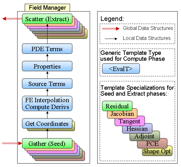
Figure 1: A schematic of the template based generic programming model for PDEs. The Gather (Seed) evaluator takes global data and copies it into local storage, seeding any embedded data types in template specialized codes. The Scatter (extract) phase does the inverse. The Compute phase can be written on the generic template type, operating on local data.

The execution of the phases is initiated by the application code and handled by the Phalanx package [18] by traversing the evaluation kernels in the directed acyclic graph. More details on the three phases for a typical finite element assembly will be described in the subsequent sections.

3.1 Finite Element Assembly Process under TBGP

Framing the finite element assembly process in terms of the template-based generic programming concept is best explained by example. Here we apply the Galerkin finite element method to a generic scalar multidimensional conservation equation (see, for example, [6])

$$\dot{u}+\nabla\cdot\mathbf{Q}+s=0,$$ (1)

where $u$ is the unknown being solved for (i.e. the degree of freedom) and $\dot{u}$ its time derivative. The flux $\mathbf{Q}$ and source term $s$ are functions of $u$, time, and position. While the exact form of the flux is not important, we comment that if the flux is strongly convecting, then additonal terms such as SUPG [12, 4] may be required to damp non-physical oscillations. To simplify the analysis, we ignore such terms here. This is valid for systems where convection is not dominant such as low Reynolds number flows or heat conduction in a solid. Equation (1) is put into variational form which, after integration by parts and ignoring boundary contributions for the sake of simplicity, yields the residual equations

$$R_{u}^{i}=\int_{\Omega}\left[\phi^{i}\dot{u}-\boldsymbol{\nabla}\phi^{i}\boldsymbol{\cdot}{\boldsymbol{Q}}+\phi^{i}s\right]\,\mathrm{d}\Omega.$$ (2)

In (2), $\Omega$ is the domain over which the problem is solved and $\phi^{i}$ are the finite element basis functions. The unknown, its time derivative, and its spatial derivative are computed using

$$u=\sum_{i=1}^{N_{u}}\phi^{i}u^{i},\dot{u}=\sum_{i=1}^{N_{u}}\phi^{i}\dot{u}^{i}$$ (3)

$$\frac{\partial u}{\partial x_{j}}=\sum_{i=1}^{N_{u}}\frac{\partial\phi^{i}}{\partial x_{j}}u^{i},$$ (4)

where $u^{i}$ are the unknown coefficients of the discretization of $u$, $x_{j}$ is the coordinate direction, and $N_{u}$ is the number of basis functions. The integrations in (2) are performed using numerical quadrature,

$$\hat{R}_{u}^{i}=\sum_{e=1}^{N_{E}}\sum_{q=1}^{N_{q}}\left[\phi^{i}\dot{u}-\boldsymbol{\nabla}\phi^{i}\boldsymbol{\cdot}{\boldsymbol{Q}}+\phi^{i}s\right]w_{q}|j|=0,$$ (5)

where $N_{E}$ is the total number of elements in the domain, $N_{q}$ is the number of quadrature points in an element for the integration order, $|j|$ is the determinant of the Jacobian of transformation from the physical space to the element reference space, and $w_{q}$ the quadrature weights.

With the finite element assembly algorithm defined by (5), the process can be redefined in terms of the gather-compute-scatter operations. The assembly algorithm in (5) loops over the elements in the domain and sums the partial contributions to form the residual equations, $\hat{R}_{u}^{i}$. The complete set of residual equations constitute the global residual, $f$. Reformulating in terms of the workset concept, the assembly process for evaluating a residual is defined as,

$$f(x)=\sum_{k=1}^{N_{w}}f_{k}=\sum_{k=1}^{N_{w}}S_{k}^{T}\bar{R}_{u_{k}}^{i}(G_{k}x).$$ (6)

Here $N_{w}$ is the number of worksets and $f_{k}$ is the partial residual associated with the finite element contributions for the elements in workset $k$. $G_{k}$ is the gather operation that maps the global solution vector, $x$, to the local solution vector for workset $k$. As mentioned above, in the software implementation, the gather routine also performs the seeding of scalar types. $S_{k}^{T}$ is the scatter operation that maps the local element residual for elements of workset $k$ into the global residual contribution, $f_{k}=S_{k}^{T}\bar{R}_{u_{k}}^{i}$. As noted above, in the software implementation, the extraction process occurs during the scatter. $\bar{R}_{u_{k}}^{i}$ are the element residual contributions to $\hat{R}_{u}^{i}$ that come from the elements in workset $k$ as a function of the local workset solution vector $G_{k}x$,

$$\bar{R}_{u_{k}}^{i}=\sum_{e=1}^{N_{e}}\sum_{q=1}^{N_{q}}\left[\phi^{i}\dot{u}-\boldsymbol{\nabla}\phi^{i}\boldsymbol{\cdot}{\boldsymbol{Q}}+\phi^{i}s\right]w_{q}|j|=0.$$ (7)

$N_{e}$ is the number of elements in workset $k$.

The important point to note is that while all of the code written above was used for evaluating a residual, the bulk of the code can now be reused for other evaluation types such as Jacobians, parameter sensitivities, stochastic residuals, etc. This is accomplished merely by writing an additional specialization for the gather, $G_{k}$, and scatter, $S_{k}^{T}$, operations only. All of the code for the residual evaluation, $\bar{R}_{u_{k}}^{i}$, is written once for a generic template argument for the scalar type and is reused for each evaluation type.

In the following sections, we now show examples and further explain each of the assembly steps.

3.2 Seed & Gather Phase: Template Specialization

In this first phase, the approach is to do the gather operation, $G_{k}$, (pulling quantities from a global vector) and the seed phase (initializing the template type for the desired embedded operation) in the same block of code. In this example, which is an adaptation of working code, the Phalanx evaluator called GatherSolution is where this operation occurs, and within the evaluateFields method in particular. As described in the previous paper [19], the Trilinos package Phalanx [18] is used to build the governing equations, where separate pieces of the computation are broken into Phalanx evaluator objects.

The field to be evaluated is called local_x, the solution vector at the local nodes of each element. It depends on global_x, which is the solution vector in the vector data layout. In Figure 2,

void GatherSolution<EvaluationType::Residual>::
evaluateFields() {
  // NOTE:: local_x is a 2D MDArray of dimension (numberOfElements,numberOfLocalNodes)
  //        of data type:  double
  for (int elem=0; elem < numberOfElements; elem++)
    for (int node=0; node < numberOfLocalNodes; node++)
      local_x(elem,node) = global_x(ConnectivityMap(elem,node));
}

Figure 2: Seed and Gather code for Residual evaluation. The ConnectivityMap function is the degree of freedom, or connectivity map, that gets the global ID from the element number and local node number. The Seed phase is trivial, just a copy of the value.

the GatherSolution class is specialized to the Residual evaluation type. This routine simply copies the values from one data structure to another with the use of a bookkeeping function ConnectivityMap. In Figure 3,

void GatherSolution<EvaluationType::Jacobian>::
evaluateFields() {
  // NOTE:: local_x is a 2D MDArray of dimension (numberOfElements,numberOfLocalNodes)
  //        of data type:  Sacado::FAD with allocated space for
  //                       numberOfLocalNodes partial derivatives.
  for (int elem=0; elem < numberOfElements; elem++) {
    for (int node=0; node < numberOfLocalNodes; node++) {
      local_x(elem,node).val() = global_x(ConnectivityMap(elem,node));
      // Loop over all nodes again, and Seed  dx/dx=I
      for (int wrt_node=0; wrt_node < numberOfLocalNodes; wrt_node++) {
        if (node == wrt_node) local_x(elem,node).dx(wrt_node) = 1.0;
        else                  local_x(elem,node).dx(wrt_node) = 0.0;
      }
    }
  }
}

Figure 3: Seed and Gather Code for Jacobian evaluation. The Gather operation is the same as the Residual calculation. The Seed phase involves local_x, which is now an automatic differentiation data type. The method local_x.val() accesses the value, and local_x.dx($i$) accessing the $i^{th}$ partial derivative. The example here assumes one equation and one unknown per local node.

the code for the GatherSolution class specialized to the Jacobian evaluation type is shown. In addition to the gather operation to load the value of $x$ into the local data structure, there is also a seed phase to initialize the partial derivatives with the identity matrix. Here, the independent variables are defined by initializing the partial derivative array of the Sacado::FAD automatic differentiation data type. Two nested loops over the local nodes are used to set $\frac{dx_{i}}{dx_{j}}$ to $1.0$ when $i=j$ and to $0.0$ otherwise.

As the number of output quantities to be produced by the finite element assembly increases (such as those defined by the rows in Table 1), so does the number of template specialized implementations of the GatherSolution object need to be written. The syntax here is dependent on the implementation in the Sacado package in Trilinos, but the concept of seeding automatic differentiation calculations is general.

3.3 Compute Phase: Generic Template

The compute phase that computes the local contributions, $\bar{R}_{u_{k}}^{i}$, for a PDE application operates on data that exists in the local element-based data structures. This code is written entirely on the generic evaluation template type EvalT. One must just write the code needed to evaluate the residual equation, but using the ScalarT data type corresponding to the evaluation type EvalT instead of raw double data type (as shown in Section 7.1 of [19]). The overloaded data type, together with specializations in the Seed and Extract phases, enable the same code to compute all manner of quantities such as the outputs in Table 1.

In this section we give two examples of the evaluateFields method of a Phalanx evaluator class. The first is shown in Figure 4 which calculates a source term in a heat equation,

$$s=\alpha+\beta u^{2},$$ (8)

where $s$ is the source term from Equation 1, $\alpha$ and $\beta$ are parameters in this model, and $u$ is the solution field. The code presupposes that the field $u$ has been computed in another evaluator and is an MDArray over elements and quadrature points. The factors $\alpha$ and $\beta$ in this example are scalar values that do not vary over the domain. (We will discuss later in Section 4.1 how to expose $\alpha$ and $\beta$ as parameters for design or analysis.) Note again that this code is templated on the generic EvalT evaluation type, and only one implementation is needed.

void SourceTerm<EvalT>::
evaluateFields() {
  // NOTE:: This evaluator depends on properties "alpha" and "beta"
  //        and scalar quantity "u" to compute the scalar source "s"
  for (int elem=0; elem < numberOfElements; elem++) {
    for (int qp=0; qp < numberOfQuadPoints; qp++) {
      source(elem,qp) += alpha + beta * u(elem,qp) * u(elem,qp);
    }
  }
}

Figure 4: Example of an evaluation kernel from the Compute phase. Note that the code is templated on the Generic EvalT evaluation type. This code will propagate the auxiliary information contained in EvalT::ScalarT data type for any of the embedded capabilities. No template specialization is needed.

For general PDE codes, it is common, and efficient, to use discretization libraries to perform common operations. For a finite element code, this includes basis function calculations, calculating the transformation between reference and physical elements, and supplying quadrature schemes. To the extent that these operations occur within the seed-compute-extract loop, they must support templating for the TBGP approach to work. In Trilinos, the Intrepid discretization library [3] serves all these roles, and was written to be templated on the generic ScalarT data type.

Figure 5 shows an example evaluator method for the final assembly of the residual equation for a heat balance. This code uses the Integrate method of the Intrepid finite element library to accumulate the summations over quadrature points of each of the four terms. The integrals are from the variational formulation of the PDEs, where the terms are matched with the Galerkin basis functions (adapted from equation (2) but using common notation for heat transfer):

$$f=\int_{\Omega}{(\mathbf{Q}\cdot\nabla\phi^{i})\,\mathrm{d}\Omega}+\int_{\Omega}{(s\phi^{i})\,\mathrm{d}\Omega}+\int_{\Omega}{(\dot{T}\phi^{i})\,\mathrm{d}\Omega}$$ (9)

where $\phi^{i}$ are the basis functions. The three terms on the right hand side correspond to the diffusive, source, and accumulation terms.

The source term $s$ in this equation can be a function of the solution, a function of the position, or a simple constant. The dependencies must be defined in the source term evaluator. However, these dependencies do not need to be described in the heat equation residual. This same piece of code will accurately propagate any derivatives that were seeded in the gather phase, and accumulated in the source term evaluator.

void HeatEquationResidual<EvalT>::
evaluateFields() {
  // NOTE:: This evaluator depends on several precomputed fields,
  //        flux, source, Tdot (time derivative),
  //        wBF (Basis Function with quadrature and transformation weights)
  //        and wGradBF (gradient of Basis Functions with weights).
  //        The result is the TResidual field, the element contribution
  //        to the heat equation residual.

  typedef Intrepid::FunctionSpaceTools FST;

  FST::integrate<ScalarT>(TResidual, flux, wGradBF);

  FST::integrate<ScalarT>(TResidual, source, wBF);

  FST::integrate<ScalarT>(TResidual, Tdot, wBF);
}

Figure 5: Evaluator for the final assembly of the heat equations. The terms correspond to those in Eq. 9, in order. The variable TResidual is being accumulated in each step. All variables are MDArrays. Depending on the template parameter EvalT and the corresponding data type ScalarT, this same block of code is used for accumulating the residual, Jacobian, or any of the output quantities listed in Table 1.

We should also note that it is possible to write template-specialized code for the compute phase. If, for instance, one would like to hand-code the Jacobian fill for efficiency, or to leave out terms for a preconditioner, once could simply write a function:

HeatEquationResidual<EvaluationType::Jacobian>::evaluateFields()

where the generic template type EvalT is replaced by the template specialized evaluation type of Jacobian.

3.4 Extract & Scatter Phase: Template Specialization

This section closely mimics Section 3.2, but with the transpose operations. Here, each local element’s contributions to the finite element residual is scattered into the global data structure. At the same time, if additional information is stored in the templated data types, it is extracted and scattered into the global linear algebra objects.

In this example, the evaluator object called ScatterResidual is where this operation occurs, and within the evaluateFields method in particular. The culmination of all the compute steps above have resulted in the computation of the field local_f, which represents the local element’s contribution, $\bar{R}_{u_{k}}^{i}$, to the global residual vector, but may also contain additional information in the ScalarT data type.

In Figure 6, the ScatterResidual class is specialized to the Residual evaluation type. This routine simply copies the values from the element data structure to the global data structure with the use of the same bookkeeping function ConnectivityMap that was used in Section 3.2. In Figure 7, the code for the ScatterResidual class specialized to the Jacobian evaluation type is shown. Here, the local, dense, stiffness matrix is extracted from the Sacado::FAD automatic differentiation data type. Two nested loops over the local nodes are used to extract $\frac{df_{i}}{dx_{j}}$ and load them into the global sparse matrix.

void ScatterResidual<EvaluationType::Residual>::
evaluateFields() {
  // NOTE:: local_f is a 2D MDArray of dimension (numberOfElements,numberOfLocalNodes)
  //        of data type:  double
  for (int elem=0; elem < numberOfElements; elem++)
    for (int node=0; node < numberOfLocalNodes; node++)
      global_f(ConnectivityMap(elem,node)) = local_f(elem,node);
}

Figure 6: Extract and Scatter Code for Residual evaluation. The ConnectivityMap function is also called the degree of freedom map, and gets the global ID from the element number and local node number. The Extract phase is trivial for this Evaluation type, just a copy of the value.

void ScatterResidual<EvaluationType::Jacobian>::
evaluateFields() {
  // NOTE:: local_f is a 2D MDArray of dimension (numberOfElements,numberOfLocalNodes)
  //        of data type:  Sacado::FAD with allocated space for
  //                       numberOfLocalNodes partial derivatives.
  for (int elem=0; elem < numberOfElements; elem++) {
    for (int node=0; node < numberOfLocalNodes; node++) {
      int row=ConnectivityMap(elem,node);
      for (int wrt_node=0; wrt_node < numberOfLocalNodes; wrt_node++) {
        int col=ConnectivityMap(elem,wrt_node);
        double val = local_f(elem,node).dx(wrt_node); //Extract df_i/dx_j
        AddSparseMatrixEntry(row,col,val);
      }
    }
  }
}

Figure 7: Extract and Scatter Code for Jacobian evaluation. The Extract phase involves local_f, which is now an Automatic Differentiation data type. The method dx($i$) on this data type accesses the $i^{th}$ partial derivative. A (fictitious) method called AddSparseMatrixEntry(int row, int col, int value) shows how this Jacobian information is scattered into the global and sparse $\frac{df}{dx}$ storage.

A set of template specialized implementations of the ScatterResidual object need to be written to match those in the GatherSolution class. Just two are shown here. These implementations are specific to the interface to the global data structures being used, which here are encapsulated in the ConnectivityMap() and AddSparseMatrixEntry() methods.

A central point to this paper, and the concept of template-based generic programming, is that the implementations in the Seed & Gather and the Extract & Scatter sections can be written agnostic to the physics being solved. While the work of correctly programming these two phases for all evaluation types is not at all trivial, the development effort is completely orthogonal to the work of adding terms to PDEs. Once a code is set up with implementations for a new evaluation type, it is there for any PDEs assembled in the compute phase.

We note that while the examples shown here are trivial, the design of the assembly engine is very general and allows for complex multiphsyics problems. In particular, unknowns are not all bound to the same basis. Fully-coupled mixed basis problems have been demonstrated with the Phalanx assembly engine. The design of each evaluator in the graph is completely controlled by the user, thus allowing for any algorithm local to the workset to be implemented.

We further note that for all of the evaluation routines above, the loops were explicitly written in the evaluator. In general, this is not ideal since it is likely to be repeated across multiple evaluators and can introduce additional points for error. These loops could be eliminated using utility functions or expression templates [28]. This will be a future area of research. Furthermore, optimizing the ordering of the nested loops and the corresponding data layouts of the field data and embedded scalar types are also areas of future research.

Finally, we note that during the design of the Phalanx package, great care was given to designing the library so that users with little C++ template experiience could easily add new physics. We feel this has been extremely successful in that there exists over 10 distinct physics applications using the TBGP packages in Trilinos. The drawback, however, is that the initial setup of the TBGP process requires a programmer with a strong background with templates. In contrast, DSL-based codes such as Sundance [16] and FEniCS [14, 15] automate the entire assembly process for users lowering the barrier for adoption. We feel that the extra work in setting up the TBGP machinery is worth the effort as we have very quickly extended the embedded analysis support to new types such as the stochastic galerkin methods.

4 Extensions to TBGP for Finite Element Code Design

The basic implementation details for template-based generic programming approach for finite element code were described in the previous section. As we have implemented this approach in application codes, we have run across many issues, and implemented solutions to them. Some of the most important of these are described in the following sections.

4.1 Infrastructure for Exposing Parameters/Properties

One of the main selling points of the template-based generic programming approach is the ability to perform design and analysis involving system parameters. Continuation, sensitivity analysis, optimization, and UQ all require that model parameters be manipulated by the analysis algorithms. These parameters are model specific, and commonly include a value of a boundary condition, a dimensionless group such as the Reynolds number, a model parameter such as an Arrhenius rate coefficient, or a shape parameter such as the radius of some cylindrical part. In this section we briefly describe our infrastructure for exposing parameters.

Infrastructure for dealing with parameters should try to meet the following design requirements: a simple interface for model developers to expose new parameters, integration into the template-base approach so derivatives with respect to parameters are captured, and seamless exposure of the parameters to design algorithms such as optimization and UQ.

The approach that has been successful in our codes has been to use the ParameterLibrary class in the Sacado package of Trilinos. This utility stores the available parameters by string name and value, and can handle the multiple data types needed by the template-based approach. The developer can register parameters in the parameter library, identified by strings, by simply calling the register method during the construction phase. To expose the $\alpha$ and $\beta$ parameters in the above Example 4 by labels “Alpha” and “Beta”, the constructor for the SourceTerm evaluator simply needs to add the lines:

parameterLibrary.registerParameter("Alpha",this);
parameterLibrary.registerParameter("Beta",this);

assuming that a parameterLibrary object is in scope. At the end of the problem construction, the parameter library can be queried for a list of registered parameters, and will include these two in addition to those registered elsewhere.

The analysis algorithms can then manipulate the values of these parameters in the ParameterLibrary. There is a choice of using a push or a pull paradigm: when the value is changed in the parameter library, is it immediately pushed to the evaluator where it will eventually be used, or is it up to the model to pull the parameter values from the parameter library when needed. We have chosen the push approach, since with this choice there is no performance penalty for exposing numerous parameters as potential design variables. Parameters are only pushed to one location, so parameters that are used in multiple evaluators must have a root evaluator where they are registered and other evaluators must have a dependency on that one.

Any evaluator class that registers a parameter must inherit from an abstract ParameterAccessor class, which has a single method called ScalarT& getValue(std::string name). Any parameter that gets registered with the ParameterLibrary needs to send a pointer to a ParameterAccessor class, so the parameter library can push new values of the parameter when manipulated by an analysis algorithm. In the example above, this is handled by the this argument in the registration call.

For this example, the getValue method can be simply implemented as shown in Figure 8, assuming parameters alpha and beta are member data of generic template type ScalarT. Sensitivities of the residual equation with respect to parameters are calculated with automatic differentiation when evaluated with the Tangent evaluation type. Like the Jacobian evaluation type, the associated Scalar data type is a Sacado::FAD type. However, the length of the derivative array is the number of parameters, and the seed and extract phases require different specializations.

ScalarT& SourceTerm<EvalT>::getValue(std::string name)
{
  if (name=="Alpha") return alpha;
  elseif (name=="Beta") return beta;
}

Figure 8: Example implementation of getValue method, which provides a hook for analysis algorithms to manipulate design parameters.

4.2 Shape Optimization: A Second Scalar Type

Quantities in the PDE assembly that might have nonzero partial derivatives with respect to an independent variable (whether it be a parameter or part of the solution vector) must be a have a templated data type. In this way, derivatives can be propagated using the object overloading approach. Constants (such as $\pi$) can be hardwired to the RealType data type to avoid the expense of propagating partial derivatives that we know are zero.

For the bulk of our calculations, the coordinates of the nodes in our finite element mesh are fixed. All the quantities that are solely a function of the coordinates, such as the basis function gradients and the mapping from an element to the reference element, can be set to RealType. However, when we began to do shape optimization, the coordinates of the node could now have nonzero derivatives with respect to the shape parameter in the Tangent (sensitivity) evaluation. To simply make all quantities that are dependent on the coordinates to be the ScalarT type would trigger an excessive amount of computations, particularly for the Jacobian calculations, where the chain rule would be propagating zeroes through a large part of the finite element assembly.

The solution was to create a second generic data type, MeshScalarT, for all the quantities that have non-zero derivatives with respect to the coordinates, but have no dependency on the solution vector. The Traits class defined in the previous paper is extended to include MeshScalarT as well as ScalarT as follows.

  struct UserTraits : public PHX::TraitsBase {

    // Scalar Types
    typedef double RealType;
    typedef Sacado::FAD FadType;

    // Evaluation Types with default scalar type
    struct Residual { typedef RealType ScalarT; typedef RealType MeshScalarT;};
    struct Jacobian { typedef FadType ScalarT;  typedef RealType MeshScalarT;};
    struct Tangent { typedef FadType ScalarT;  typedef FadType MeshScalarT;};
    .
    .
    .
  }

If, in the future we decide to do a moving mesh problem, such as thermo-elasticity, where the coordinate vector for the heat equation does depend on the current displacement field as calculated in the elasticity equation, then the Jacobian evaluation could be switched in this traits class to have typedef FadType MeshScalarT. Automatically, the code would calculate the accurate Jacobian for the fully coupled moving mesh formulation.

While it can be complicated to pick the correct data type for all quantities with this approach, the Sacado implementation of these data types has a useful feature. The code will not compile if you attempt to assign a derivative data type to a real type. The casting away of derivative information must be done explicitly, and can not be done by accident. This is illustrated in the following code fragment, as annotated by the comments.

RealType r=1.0;
FadType f=2.5;
f = r;  //Allowed. All derivatives set to zero.
r = f;  //Compiler will report an error.

4.3 Template Infrastructure

Template-based generic programming places a number of additional requirements on the code base. Building and manipulating the objects can be intrusive. Additionally the compile times can be excessive as more and more template types are added to the infrastructure. Here we address these issues.

4.3.1 Extensible Infrastructure

The infrastructure for a template-based assembly process must be designed for extensibility. The addition of new evaluation types and/or scalar types should be minimally invasive to the code. To support this requirement, a template manager class has been developed to automate the construction and manipulation of a templated class given a list of template types.

A template manager instantiates a particular class for each template type using a user supplied factory for the class. The instantiated objects are stored in a std::vector inside the manager. To be stored as a vector, the class being instantiated must inherit from a non-templated base class. Once the objects are instantiated, the template manager provides functionality similar to a std::vector. It can return iterators to the base class objects. It allows for random access based on a template type using templated accessor methods, returning an object of either the base or derived class.

The list of types a template manager must build is fixed at compile time through the use of template metaprogramming techniques [1] implemented in the Boost MPL library [5] and Sacado [21]. These types are defined in a “traits” class. This object is discussed in detail in [19].

We note that the template manager described here is a simplified version of the tuple manipulation tools supplied by the Boost Fusion library [5]. In the future, we plan to transition our code to using the Fusion library.

4.3.2 Compile Time Efficiency

For each class templated on an evaluation type, the compiler must build the object code for each of the template types. This can result in extremely long compile times even for very minor code changes. For that reason explicit template instantiation is highly recommended for all classes that are templated on an evaluation type. In our experience, not all compilers can support explicit instantiation. Therefore both the inclusion model and explicit template instantiation are supported in our objects (see Chapter 6 of [27] for more details) .

The downside to such a system is that for each class that implements explicit instantiation, the declaration and definition must be split into separate header files and a third (file.cpp) file must also be added to the code base.

4.4 Incorporating Non-Templated Third-Party Code

In some situations, third-party code may provide non-template based implementations of some analysis evaluations. For example, it is straightforward to differentiate some Fortran codes with source transformation tools such as ADIFOR [2] to provide analytic evaluations for first and higher derivatives. However clearly the resulting derivative code does not use the template-based procedure or the Sacado operator overloading library. Similarly some third-party libraries have hand-coded derivatives. In either case, some mechanism is necessary to translate the derivative evaluation governed by Sacado into one that is provided by the third-party library. Providing such a translation is a relatively straightforward procedure using the template specialization techniques already discussed. Briefly, a Phalanx evaluator should be written that wraps the third-party code into the Phalanx evaluation hierarchy. This evaluator can then be specialized for each evaluation type that the third-party library provides a mechanism for evaluating. This specialization extracts the requisite information from the corresponding scalar type (e.g., derivative values) and copies them into whatever data structure is specified by the library for evaluating those quantities. In some situations, the layout of the data in the given scalar type matches the layout required by the library, in which case a copy is not necessary (e.g., Sacado provides a forward AD data type with a layout that matches the layout required by ADIFOR, in which case a pointer to the derivative values is all that needs to be extracted). However this is not always the case, so in some situations a copy is necessary.

Such an approach will work for all evaluation types that the third-party library provides some mechanism for evaluating. However clearly situations can arise where the library provides no mechanism for certain evaluation types. In this case the specializations must be written in such a way as to generate the required information non-intrusively. For example, if the library does not provide derivatives, these can be approximated through a finite-differencing scheme. In a Jacobian evaluation for example, the Jacobian specialization for the evaluator for this library would make several calls to the library for each perturbation of the input data for the library, combine these derivatives with those from the inputs (dependent fields) for the evaluator (using the chain rule) and place them in the derivative arrays corresponding to the outputs (evaluated fields) of the evaluator. Similarly polynomial chaos expansions of non-templated code can be computed through non-intrusive spectral projection [23].

4.5 Mesh Morphing and Importing Coordinate Derivatives

The shape optimization capability that will be demonstrated in Section 5 requires sensitivities of the residual equation with respect to shape parameters. Our implementation uses an external library for moving the mesh coordinates as a function of shape parameters, a.k.a. mesh morphing. This is an active research area, and a paper has just been prepared detailing six different approaches on a variety of applications [26].

Briefly, the desired capability is for the application code to be able to manipulate shape parameters, such as a length or curvature of part of a solid model, and for the mesh morphing utility to provide a mesh that conforms to that geometry. To avoid changes in data structures and discontinuities in an objective function calculation, it is desirable for the mesh topology, or connectivity, to stay fixed. The algorithm must find a balance between maintaining good mesh quality and preserving the grading of the original mesh, such as anisotropy in the mesh designed to capture a boundary layer. Large shape changes that require remeshing are beyond the scope of this work, and would need to be accommodated by remeshing and restarting the optimization run.

A variety of mesh morphing algorithms have been developed and investigated. At one end of the spectrum is the smoothing approach, where the surface nodes are moved to accommodate the new shape parameters and the resulting mesh is smoothed until the elements regain acceptable quality. At the other end of the spectrum is the FEMWARP algorithm [25], where a finite element projection is used to warp the mesh, requiring a global linear solve to determine the new node locations. In this paper, we have used a weighted residual method, where the new node coordinates are based on how boundary nodes in their neighborhood have moved. We chose to always morph the mesh from the original meshed configuration to the chosen configuration, even if an intermediate mesh was already computed at nearby shape parameters, so that the new mesh was uniquely defined by the shape parameters.

Since the mesh morphing algorithm is not a local calculation on each element but operates across the entire mesh at one time, the derivatives cannot be calculated within a Phalanx evaluator using the template-based approach, nor using the methods described in Section 4.4.

Our approach for calculating sensitivities of the residual vector $f$ with respect to shape parameters $p$ is to use the chain rule,

$$\frac{\partial f}{\partial p}=\frac{\partial f}{\partial X}\frac{\partial X}{\partial p}.$$ (10)

where $X$ is the coordinate vector. Outside of the seed-compute-extract section of templated code, we pre-calculate the mesh sensitivities $\frac{\partial X}{\partial p}$ with a finite difference algorithm around the mesh morphing algorithm. This multi-vector is fed into the residual calculation as global data.

As part of the typical assembly, there is a gatherCoordinates evaluator that takes the coordinate vector from the mesh database and gathers it into the local element-based MDArray data structure. For shape sensitivities, the coordinate vector is a Sacado::FAD data type, and the gather operation not only imports the values of the coordinates, but also seeds the derivative components from the pre-calculated $\frac{\partial X}{\partial p}$ vectors. This is shown schematically in Figure 1, where the GatherCoordinates box is shown to have a template specialized version for shape optimization in addition to a generic implementation for all other evaluation types. When the rest of the calculation proceeds, the directional derivative of $\frac{\partial f}{\partial X}$ in the direction of $\frac{\partial X}{\partial p}$ is computed. The same implementation for extracting $\frac{\partial f}{\partial p}$ works for this case as when $p$ is a set of model parameters as described in Section 4.1.

5 Demonstration: Sliding Electromagnetic Contact

The template-based generic programming approach is demonstrated here on a prototype 3D PDE application: the sliding electromagnetic contact problem. The geometry of this problem is shown in Figure 9, where, for the nominal design, this 2D geometry is simply extruded into the third dimension. A slider (light blue) is situated between two conductors (green and yellow) with some given shapes of the contact pads (thin red and blue regions). When a potential difference ($\psi$) over the device is prescribed, an electrical current flows through system in the general direction of the dashed red line. The electrical current generates a magnetic field that in turn propels the slider forward. In addition, the current generates heat.

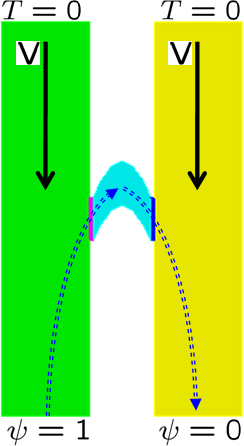
Figure 9: A front view of the geometry for the sliding electromagnetic contact application. The imposed gradient in potential $\psi$ causes electric current, Joule heating, and a magnetic field that propels the slider (which is not currently modeled).

The design problem to be investigated is to find the shape of the slider, with a given volume, that minimizes the maximum temperature achieved inside of it.

5.1 Governing Equations and Objective Function

In this demonstration, we simplify the system by decoupling the magnetics, and solve a quasi-steady model where the slider velocity v is given. The model is then reduced to two coupled PDEs. The first is a potential equation for the electric potential $\psi$. The second is a heat balance that accounts for conduction, convection, and Joule heating source term that depends on the current $\nabla\psi$:

$$-\nabla\cdot\sigma\nabla\psi = 0,$$ (11)

$$-\nabla\cdot\kappa\nabla T-{\mbox{v}}\cdot\nabla T = \sigma(\nabla\psi)^{2}.$$ (12)

The electrical conductivity, $\sigma$, varies as a function of the local temperature field based on a simplified version of Knoepfel’s model [13],

$$\sigma(T) = {\sigma_{0}}/[1+\beta(T-T_{0})],$$ (13)

where $\sigma_{0}$ can take different values in the slider, the conductor, and in the pads ($\sigma^{p}_{0}$). This dependency results in a coupled pair of equations.

By choosing the frame of reference that stays with the slider, we impose a fixed convective velocity $\mbox{v}_{0}$ in the beams, and $\mbox{v}=0$ in the slider. The Dirichlet boundary conditions for the potential and temperature are shown in Figure 9, with all others being natural boundary conditions. Since these equations and geometry are symmetric about the mid plane (a vertical line in this figure), we only solve for half of the geometry and impose $\psi=0.5$ along this axis.

This PDE model was implemented using Phalanx evaluators. By specifying the dependencies with the evaluators, such as $\sigma(T)$, the evaluation tree is automatically constructed. The full graph for this problem is shown in Figure 10. As with the ODE example in the previous paper [19], only the Gather and Scatter functions need to be written with template specialization for the Seed and Extract phases. All the intermediate Compute quantities can be written once on a generic evaluation type.

As an example of how to interpret this graph: the oval marked $T_{q}$ computes the temperature field at the quadrature points using the Basis Functions and $T_{n}$, the Temperature field at the nodes (implementing Equation 3); $T_{q}$ is subsequently used to compute $\kappa$ and $\sigma$ in another evaluator (which implements Equation 13).

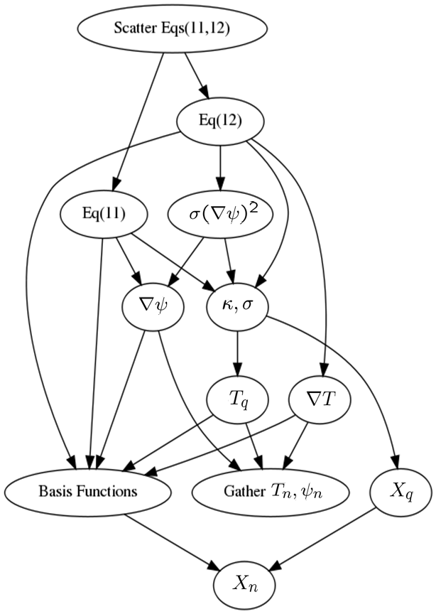
Figure 10: The dependency graph for the Phalanx evaluators that build the thermo-electric equation set is shown. Each box represents a separate class. The quantities at the bottom must be computed before those above. Derivatives are automatically propagated by the chain rule using the Sacado Automatic Differentiation data types. Here $X$ is the coordinate vector, $T$ the temperature, and $\psi$ the potential, and subscript $n$ and $q$ indicating to node and quadrature point data.

The objective function $g$, which is to be minimized by the design problem, is simply

$$g(\psi,T)=\|T\|_{\infty}.$$ (14)

The design parameters $p$ modify the shape of the slider. Its shape is fixed to match the rectangular pads at each end, and its volume is fixed to be that of the rectangular box between them. In between, the shape is allowed to vary parabolically. For a one-parameter optimization problem, the matched parabolic profiles of the top and bottom of the slider are free to vary by a single maximum deflection parameter. Because of the symmetry of the problem, this defines the parabola. For two-parameter optimization problem, these two parabolas are allowed to vary independently and a third, the bulge of the slider out of the plane of the figure, is adjusted so that the volume constraint is met.

5.2 Gradient-based Optimization

The optimization problem is solved using a gradient-based optimization algorithm from the Dakota framework. Dakota can be built as part of Trilinos using the build system and adaptors in the TriKota package.

The goal is to minimize the objective function $g(p)$ from Equation 14 as a function of the shape parameters $p$. In addition, the problem is constrained so that the discretized PDEs are satisfied, $f(x)=0$ where $f$ represents the finite element residuals for the equation set specified in Equations 11–12 and the solution vector $x$ is the combined vector of the discretized potential and temperature fields. The shape parameters do not appear explicitly in the objective function, or even in the governing equations (11–12), but instead effect the geometry of the problem. They appear in the discretization, and can be written as $f(x,X(p)))$, where $X$ is the vector of coordinates of nodes in the mesh.

In addition to the objective function $g(p)$, the gradient-based algorithm depends on the reduced gradient of the objective function with respect to the parameters. The formula for this term can be expanded as,

$$\frac{dg}{dp}=\frac{\partial g}{\partial p}-{\frac{\partial g}{\partial x}}^{T}{\frac{\partial f}{\partial x}}^{-1}\frac{\partial f}{\partial X}\frac{dX}{dp}.$$ (15)

Each of these terms is computed in a different way. Starting at the end, the multi-vector $X_{p}=\frac{dX}{dp}$ is computed with finite differences around the mesh morphing algorithm, as described in Section 4.5. The sensitivity of the residual vector with respect to the shape parameters is the directional derivative $\frac{\partial f}{\partial X}$ in the direction $X_{p}$. This is computed using Automatic Differentiation using the infrastructure described in Section 4.5, where the Sacado automatic derivative data type for the coordinate vector $X$ is seeded with the derivative vectors $X_{p}$. The result is a multi-vector $f_{p}$.

The Jacobian matrix $\frac{\partial f}{\partial x}$ is computed with automatic differentiation. All the Sacado data types are allocated with derivative arrays of length $16$, which is the number of independent variables in a hexahedral element with trilinear basis functions and two degrees of freedom per node. The local element solution vector $x$ is seeded with $\frac{\partial x_{i}}{\partial x_{j}}=1$ when $i=j$. The action of the inverse of the Jacobian on $f_{p}$ is performed with a preconditioned iterative linear solver using the Belos and Ifpack packages in Trilinos.

The gradient of the objective function $\frac{\partial g}{\partial x}$ is computed by hand, since $g$ is the max operator on the half of $x$ corresponding to the temperature unknown. The non-differentiability of the max operator with respect to changes in parameter can in general be an issue. However, no problems were encountered in this application since the location of the maximum did nor move significantly over itrations. Finally, the term $\frac{\partial g}{\partial p}$ was identically zero because the parameters did not appear explicitly in the objective function.

First, a one-parameter optimization problem was run to find the parabolic deflection of the top and bottom of the slider that minimized the maximum temperature. In addition to the gradient-based optimization algorithm described above, a continuation run was performed using the LOCA package [24] in Trilinos. The results are shown in Figure 11. The continuation run shows the smooth response surface for a wide range if deflections, both positive and negative. The optimization iteration rapidly converges to the minimum. The optimum occurs for a small positive value of the deflection parameter, corresponding to a shape that is slightly arched upwards but rather near the nominal shape of a rectangular box.

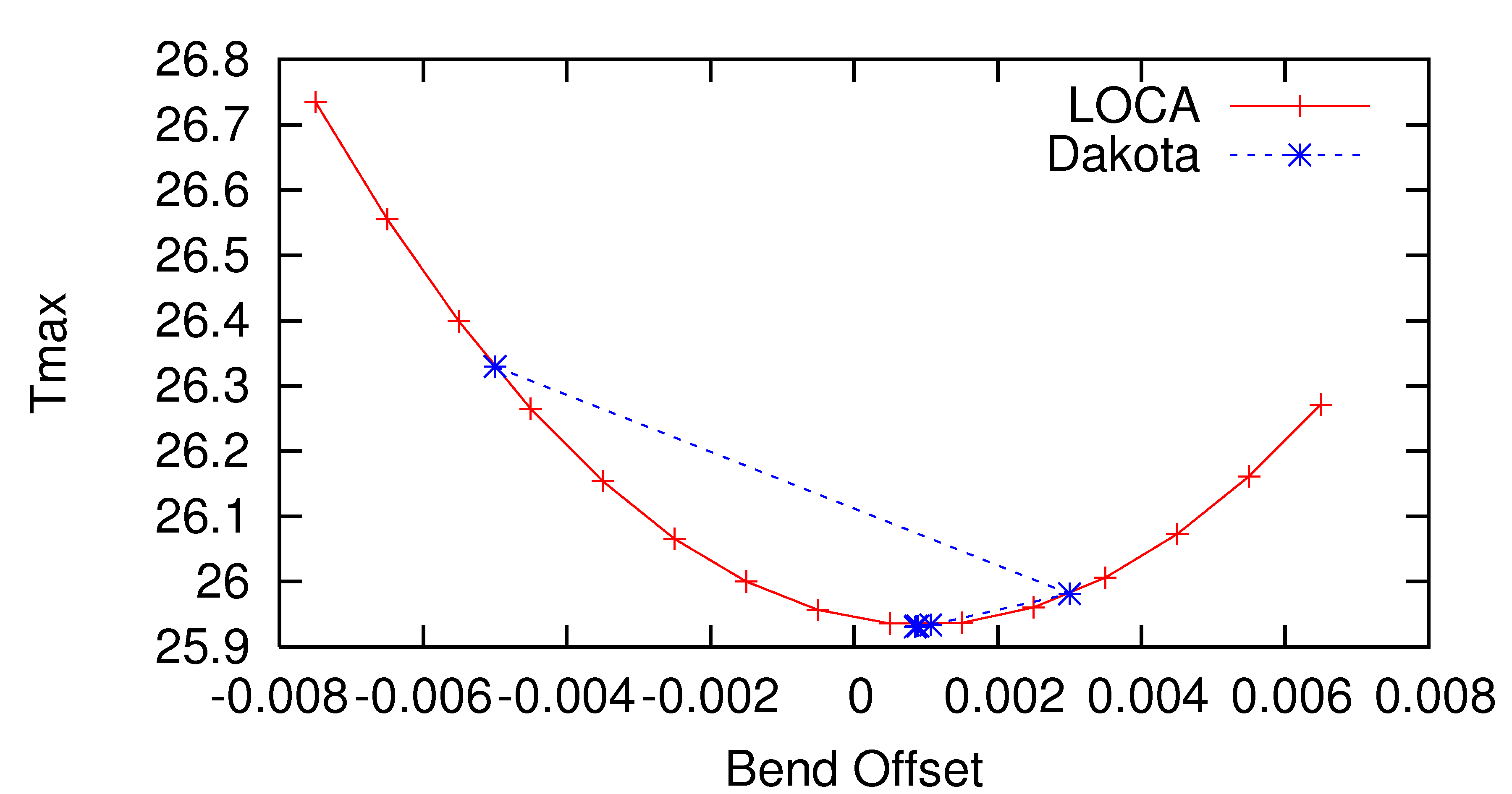
Figure 11: Results for a continuation run with LOCA and a minimization run using Dakota, for a one-parameter shape optimization problem.

A two-parameter optimization run was also performed, where the top and bottom parabolas were freed to vary independently, and the bulge of the slider was adjusted to conserve the volume of the mesh. Figure 12 shows the initial configuration, with a rather arched bottom surface, and nearly flat upper surfaces, and a moderate bulge. The optimal shape is shown in Figure 13. As with the one-parameter case, the optimal shape was found to be close to a rectangular box. The temperature contouring of the two figures, which share a color map, shows a noticeable reduction in the temperature at the optimal shape.

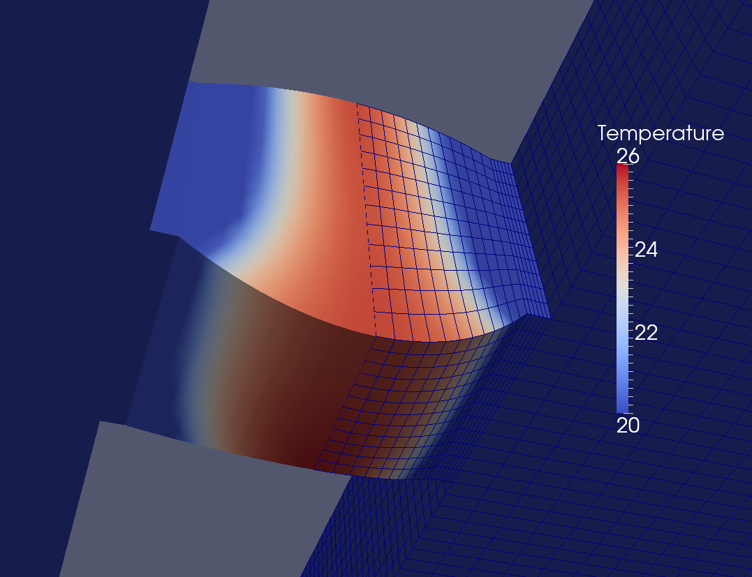
Figure 12: Initial mesh configuration and steady-state temperature profiles for the two-parameter optimization problem. The deflections of the top and bottom surface of the slider are varied independently, and the deflection (bulge) out of the plane is chosen to constrain the volume to that of a rectangular brick.

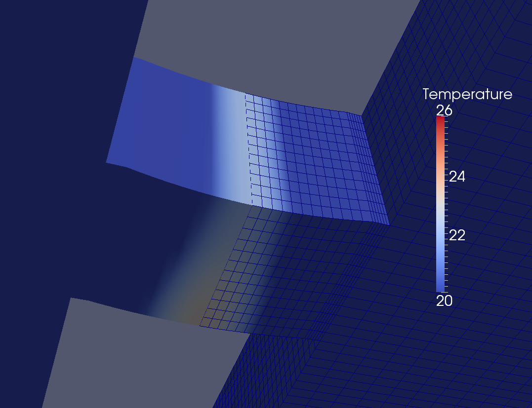
Figure 13: Final configuration and color map for the two-parameter optimization problem. The maximum temperature was significantly decreased.

5.3 UQ Results

In addition to optimization runs, embedded uncertainty quantification was performed on the same model. The ScalarT data type for the stochastic Galerkin residual evaluation hold polynomial coefficients for the expansion of all quantities with a spectral basis. By nesting the stochastic Galerkin and Automatic Differentiation data types, a Jacobian for the stochastic Galerkin expansions can also be calculated. The Seed and Extract phases of this computation, as well as the subsequent nonlinear solve of the stochastic FEM system required significant development. However, with the template-based generic programming approach, this work is completely orthogonal to the implementation of the PDEs. So, there was no additional coding needed to perform embedded UQ for this application over that needed for the residuals for the governing equations  (11–12).

As a demonstration, we chose the electrical conductivity in the pad ${\sigma^{p}_{0}}$ as the uncertain variable. The pad region is the thin rectangular region at the edge of the slider with fixed shape. In this run, ${\sigma^{p}_{0}}$ was chosen to be a uniform distribution within $15$ of the nominal value of $35$,

$${\sigma^{p}_{0}}=[35.0P_{0}(\xi)+15.0P_{1}(\xi)].$$ (16)

Here, the $P$ variables are Legendre polynomials. The computation was run with degree-3 polynomial basis. A Newton iteration was performed on the nonlinear system from the discretized 4D domain (3D FEM in space + 1 Stochastic Dimension with a spectral basis). The resulting probability distribution on the maximum temperature unknown was computed to be

$$T_{Max}=25.87P_{0}(\xi)+0.61P_{1}(\xi)-0.17P_{2}(\xi)+0.04P_{3}(\xi).$$ (17)

Figure 14 shows the mean temperature profile for this distribution. Figure 15 show the variation of the temperature with respect to this parameter. (Note the reduced range of the color bar.) The results show that the variation of the electrical conductivity in the pad region has a large effect on the temperature in the middle of the slider (which has a large dependence on the total current), and not in the pad region itself (which is strongly controlled by the convective cooling from the beam due to the moving frame of reference).

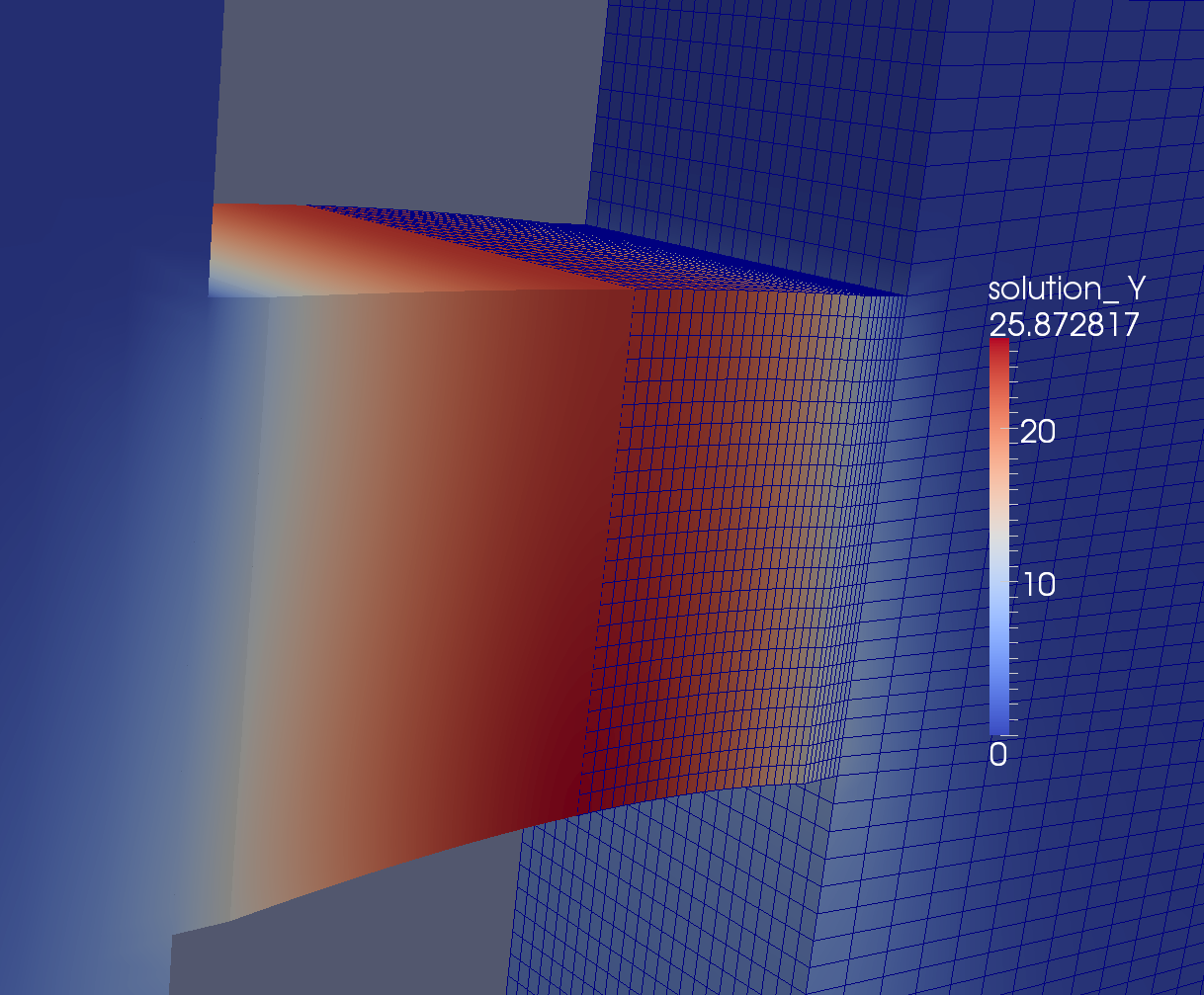
Figure 14: The results of an embedded uncertainty quantification using Stokhos. The electrical conductivity in the thin pad region is given as a distribution. In this figure, the temperature profile for the mean solution is shown.

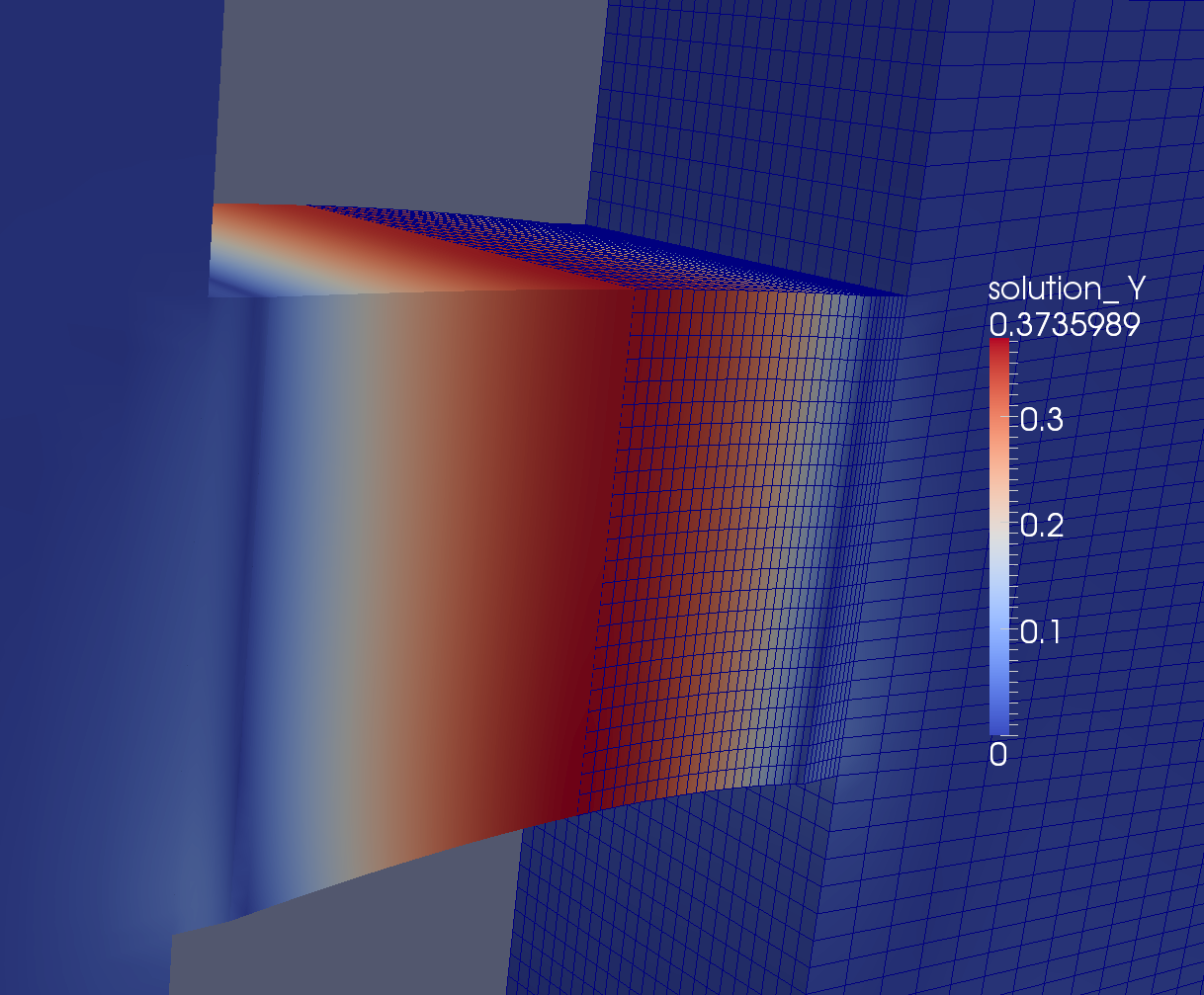
Figure 15: The variation in the temperature field is shown, for the same embedded uncertainty quantification calculation as the previous figure.

6 Conclusions

In this paper, we have related our experience in using the template-based generic programming (TBGP) approach for PDEs in a finite element code. We have used this approach at a local element level, where the dependencies for Jacobian evaluations are small and dense. By combining the Gather phase of a finite element calculation with the Seed phase of the TBGP approach, and the Scatter with Extract, the infrastructure for TBGP is well contained. Once this infrastructure is in place, transformational analysis capabilities such as optimization and embedded UQ are immediately available for any new PDE modes that are implemented.

We have also presented some of the implementation details in our approach. This includes infrastructure for dealing with parameters, for dealing with a templated code stack, and dealing with non-templated code. We demonstrated this approach on an example sliding electromagnetic contact problem, which is a pair of coupled nonlinear steady-state equations. We performed optimization algorithms with embedded gradients, and also embedded Stochastic Finite Element calculations.

As this paper is to appear in a special issue along with other Trilinos capabilities, we would like to mention explicitly which Trilinos packages (underlined) were used in these calculations. This paper centered on the use of Phalanx assembly engine, Sacado for automatic differentiation, and Stokhos for embedded UQ. For linear algebra, we used the Epetra data structures, Ifpack preconditioners, and Belos iterative solver. The linear algebra was accessed through the Stratimikos linear algebra strategy layer using the Thyra abstraction layer. The STK Mesh package was used for the parallel mesh database, and the STK IO packages, together with Ioss, Exodus, and SEACAS were used for IO and partitioning of the mesh. The Intrepid package was used for the finite element discretization, operating on multidimensional arrays from the Shards package. The utility packages Teuchos was used for parameter list specification and reference-counted memory management.

The Piro package managed the solver and analysis algorithms, and makes heavy use of the EpetraExt Model Evaluator abstraction. Piro in turn calls the NOX nonlinear solver, the LOCA library of continuation algorithms, the TriKota interface to the Dakota optimization algorithms, and Stokhos for presenting the stochastic Galerkin system as a single nonlinear problem. These results also relied on several products outside of Trilinos, including the Cubit mesh generator and associated mesh morphing software, the Dakota framework, ParaView visualization package and netcdf mesh I/O library.

References

- Abrahams and Gurtovoy [2004] D. Abrahams and A. Gurtovoy. C++ Template Metaprogramming: Concepts, Tools, and Techniques from Boost and Beyond. Addison-Wesley, 2004.
- Bischof et al. [1996] C. H. Bischof, A. Carle, P. Khademi, and A. Mauer. ADIFOR 2.0: Automatic differentiation of Fortran 77 programs. IEEE Computational Science & Engineering, 3(3):18–32, 1996.
- Bochev et al. [2012] P. Bochev, H. Edwards, R. Kirby, K. Peterson, and D. Ridzal. Solving pdes with intrepid. Scientific Programming, In print., 2012.
- Brooks and Hughes [1982] A. N. Brooks and T. Hughes. Streamline upwind/petrov-galerkin formulations for convection dominated flows with particular emphasis on the incompressible Navier-stokes equations. Comp. Meth. Appl. Mech. and Eng., 32:199–259, 1982.
- Dawes and Abrahams [2011] B. Dawes and D. Abrahams. http://www.boost.org, 2011.
- Donea and Huerta [2003] J. Donea and A. Huerta. Finite Element Methhods for Flow Problems. Wiley, 2003.
- Edwards [2011] H. C. Edwards. http://trilinos.sandia.gov/packages/shards/, 2011.
- Ghanem and Spanos [1990] R. Ghanem and P. D. Spanos. Polynomial chaos in stochastic finite elements. Journal of Applied Mechanics, 57, Jan 1990.
- Ghanem and Spanos [1991] R. G. Ghanem and P. D. Spanos. Stochastic finite elements: a spectral approach. Springer-Verlag, New York, 1991. ISBN 0-387-97456-3.
- Griewank [2000] A. Griewank. Evaluating Derivatives: Principles and Techniques of Algorithmic Differentiation. Number 19 in Frontiers in Appl. Math. SIAM, Philadelphia, PA, 2000. ISBN 0–89871–451–6.
- Heroux et al. [2005] M. A. Heroux, R. A. Bartlett, V. E. Howle, R. J. Hoekstra, J. J. Hu, T. G. Kolda, R. B. Lehoucq, K. R. Long, R. P. Pawlowski, E. T. Phipps, A. G. Salinger, H. K. Thornquist, R. S. Tuminaro, J. M. Willenbring, A. B. Williams, and K. S. Stanley. An overview of the Trilinos package. ACM Trans. Math. Softw., 31(3), 2005. http://trilinos.sandia.gov/.
- Hughes and Brooks [1979] T. Hughes and A. N. Brooks. A multidimensional upwind scheme with no cross-wind diffusion. in T.J.R. Hughes (ed.), Finite Element Methods for Convection Dominated Flows, AMD Vol. 34, ASME, New York 19-35, 1979.
- Knoepfel [1970] H. Knoepfel. Pulsed high magnetic fields: Physical Effects and Generation Methods Concerning Pulsed Fields Up to the Megaoersted Level. North-Holland Publishing Company, Amsterdam, 1970.
- Logg [2007] A. Logg. Automating the finite element method. Arch. Comput. Methods Eng., 14(2):93–138, 2007.
- Logg et al. [2012] A. Logg, K.-A. Mardal, G. N. Wells, et al. Automated Solution of Differential Equations by the Finite Element Method. Springer, 2012. ISBN 978-3-642-23098-1.
- Long et al. [2010] K. Long, R. Kirby, and B. van Bloemen Waanders. Unified embedded parallel finite element computations via software-based frechet differentiation. SIAM J. Sci. Comput., 32(6):3323–3351, 2010.
- of a Unified C++ Implementation of the Finite et al. [2007] L. O. of a Unified C++ Implementation of the Finite, D. Spectral Element Methods in 1D, and 3D. In Applied Parallel Computing. State of the Art in Scientific Computing, volume 4699 of Lecture Notes in Computer Science, pages 712–721. Springer, 2007.
- Pawlowski [2011] R. P. Pawlowski. http://trilinos.sandia.gov/packages/phalanx/, 2011.
- Pawlowski et al. [2011] R. P. Pawlowski, E. T. Phipps, and A. G. Salinger. Automating embedded analysis capabilities and managing software complexity in multiphysics simulation part I: template-based generic programming. Scientific Programming, 2011. In press.
- Phipps and Pawlowski [2012] E. Phipps and R. Pawlowski. Efficient expression templates for operator overloading-based automatic differentiation. In S. Forth, P. Hovland, E.Phipps, J. Utke, and A. Walther, editors, Recent Advances in Algorithmic Differentiation. Springer, 2012.
- Phipps [2011] E. T. Phipps. http://trilinos.sandia.gov/packages/sacado/, 2011.
- Prud’Homme [2006] C. Prud’Homme. A domain specific embedded language in C++ for automatic differentiation, projection, integration and variational formulations. Scientific Programming, 14(2):81–110, 2006.
- Reagan et al. [2003] M. Reagan, H. Najm, R. Ghanem, and O. Knio. Uncertainty quantification in reacting-flow simulations through non-intrusive spectral projection. Combustion and Flame, 132(3):545–555, Jan 2003. doi: 10.1016/S0010-2180(02)00503-5.
- Salinger et al. [2005] A. G. Salinger, E. A. Burroughs, R. P. Pawlowski, E. T. Phipps, and L. A. Romero. Bifurcation tracking algorithms and software for large scale applications. Int J Bifurcat Chaos, 15(3):1015–1032, 2005.
- Shontz and Vavasis [2010] S. M. Shontz and S. A. Vavasis. Analysis of and workarounds for element rever- sal for a finite element-based algorithm for warping triangular and tetrahedral meshes. BIT Numerical Mathematics, 50:863–884, 2010.
- Staten et al. [2011] M. L. Staten, S. J. Owen, S. M. Shontz, A. G. Salinger, and T. S. Coffey. A comparison of mesh morphing methods for 3D shape optimization. Proceedings of the 20th International Meshing Rountable, Oct. 23–26 2011. Submitted.
- Vandevoorde and Josuttis [2003] D. Vandevoorde and N. M. Josuttis. C++ Templates, The Complete Guide. Addison-Wesley, 2003.
- Veldhuizen [1995] T. Veldhuizen. Expression templates. C++ Report, 7(5):26–31, 1995.
- Wiener [1938] N. Wiener. The homogeneous chaos. Am J Math, 60:897–936, Jan 1938.
- Xiu and Karniadakis [2002] D. Xiu and G. Karniadakis. The wiener-askey polynomial chaos for stochastic differential equations. Siam J Sci Comput, 24(2):619–644, Jan 2002.