The Green Bank Telescope HII Region Discovery Survey:
III. Kinematic Distances

Abstract

Using the H I Emission/Absorption method, we resolve the kinematic distance ambiguity and derive distances for 149 of 182 (82%) H II regions discovered by the Green Bank Telescope H II Region Discovery Survey (GBT HRDS). The HRDS is an X-band (9 GHz, 3 cm) GBT survey of 448 previously unknown H II regions in radio recombination line and radio continuum emission. Here we focus on HRDS sources from $67\arcdeg\geq\ell\geq 18\arcdeg$, where kinematic distances are more reliable. The 25 HRDS sources in this zone that have negative recombination line velocities are unambiguously beyond the orbit of the Sun, up to 20 kpc distant. They are the most distant H II regions yet discovered. We find that 61% of HRDS sources are located at the far distance, 31% at the tangent point distance, and only 7% at the near distance. “Bubble” H II regions are not preferentially at the near distance (as was assumed previously) but average 10 kpc from the Sun. The HRDS nebulae, when combined with a large sample of H II regions with previously known distances, show evidence of spiral structure in two circular arc segments of mean Galactocentric radii of 4.25 and 6.0 kpc. We perform a thorough uncertainty analysis to analyze the effect of using different rotation curves, streaming motions, and a change to the Solar circular rotation speed. The median distance uncertainty for our sample of H II regions is only 0.5 kpc, or 5%. This is significantly less than the median difference between the near and far kinematic distances, 6 kpc. The basic Galactic structure results are unchanged after considering these sources of uncertainty.

1 Introduction

H II regions, the zones of ionized gas surrounding massive OB stars, have been instrumental to our understanding of the star formation history, structure, and composition of our Milky Way Galaxy. While there are many extant catalogs of H II regions, distance information is frequently lacking. Accurate distances are required to turn the measured properties of flux and angular size into the physical properties of luminosity and physical size. Because OB stars have very brief lifetimes, H II regions trace star formation at the present epoch. They therefore are found only in locations of active star formation, primarily in spiral arms. Their chemical composition is that of the present-day interstellar medium, after billions of years of stellar processing. Distances are required if we are to use H II regions to trace Galactic structure or to learn about the chemical evolution of our Galaxy.

Measured radial velocities can be used to compute kinematic distances using a rotation curve model for the Galaxy. Rotation curves usually assume circular rotation about the Galactic center such that a model radial velocity is a function only of its Galactocentric distance. Galactic rotation curves have in general been derived using either CO (e.g., Clemens, 1985) or H I (e.g., Burton & Gordon, 1978). The different tracers employed and the different methodologies used to derive the rotation curves from measured velocity fields cause slightly different results.

Spectro-photometric distances (e.g., Russeil et al., 2007) and trigonometric parallax of associated masers (e.g., Reid et al., 2009) are potentially more accurate methods for calculating Galactic H II region distances compared to kinematic distances. Distances derived using maser parallax measurements typically have low uncertainties compared to kinematic distances. Reid et al. (2009) quote an average uncertainty of 10% for distances of 10 kpc and found for some sources discrepancies of over a factor of 2 between the kinematic and the maser parallax distances. In an extreme case, G9.62+0.20 has near and far kinematic distances of $\sim 0.5$ kpc and $\sim 16$ kpc, respectively, and Sanna et al. (2009) find a maser parallax distance of 5.2 kpc. The Galactic location of this source within 10$\,{}^{\circ}$ of the Galactic center direction, however, implies a priori that kinematic distances are not reliable.

The Green Bank Telescope H II region discovery survey (GBT HRDS; Bania et al., 2010; Anderson et al., 2011) discovered 448 Galactic H II regions by measuring their radio recombination line (RRL) velocities and radio continuum emission. The HRDS sources are found over $67\,^{\circ}\geq\ell\geq 343\,^{\circ}$, $|b|\leq 1\arcdeg$ and have doubled the number of previously known H II regions in this zone. Little is known about many of these regions.

Only kinematic distances are possible if we are to derive distances to the majority of the HRDS sample. One must locate the exciting star(s) in the optical or near infrared and assign a spectral type to derive a spectro-photometric distance. This is in general not possible for HRDS sources due to extinction as few of the HRDS nebulae are optically visible. Maser parallax distances rely on measurements using Very Long Baseline Interferometry (VLBI) of bright maser sources associated with massive star forming regions. Such maser spots are not uncommon, but are not present for all star-forming regions. Only about 10% of HRDS sources are associated with detected maser emission (Anderson et al., 2011). Our group just led an unsuccessful effort to find 12 GHz methanol masers associated with a sample of distant HRDS targets with the GBT (Anderson et al., 2012, in prep.).

Most HRDS sources lie in the portion of the Galaxy interior to the Solar orbit, the “inner Galaxy.” Each measured inner Galaxy velocity corresponds to two distinct kinematic distances, a near and a far distance. This problem is known as the kinematic distance ambiguity (KDA). Measured velocities for first-quadrant sources in the inner Galaxy increase with distance from the Sun until the tangent point, which is the location where the radial velocity is at a maximum along a given line of sight. Beyond the tangent point, radial velocities decrease. The near and far distance are spaced evenly along the line of sight about the tangent point. There are two cases over the Galactic range of the HRDS where there is no KDA: 1) sources whose velocity is the same as the tangent point velocity and 2) sources whose velocity places them unambiguously beyond the orbit of the Sun. In the first Galactic quadrant, sources beyond the orbit of the Sun have negative velocities whereas in the fourth Galactic quadrant the same is true for sources with positive velocities.

There are two common methods one can use to resolve the KDA for Galactic H II regions. Both of these methods involve the detection of a spectral line in absorption from foreground material in the direction of an H II region. H II regions emit broadband thermal continuum radiation and an absorption signal may be detected for any spectral line originating from foreground material with a lower brightness temperature than that of the H II region. The most robust such method uses H I as the absorbing material. This method is called the H I emission/absorption (H I E/A) method (Kuchar & Bania, 1994; Kolpak et al., 2003; Anderson & Bania, 2009; Urquhart et al., 2012) and it relies on the detection of H I absorption at 21 cm from the continuum emission of an H II region. A similar method uses intervening ${\rm H_{2}CO}$ clouds instead of H I to search for an absorption signal (Wilson, 1972; Downes et al., 1980; Araya et al., 2002; Watson et al., 2003; Sewilo et al., 2004). Because there is less ${\rm H_{2}CO}$ compared to H I, this method will more often resolve the KDA incorrectly and is applicable to a smaller number of H II regions. Along a given line of sight Watson et al. (2003) estimate that on average there is one ${\rm H_{2}CO}$ cloud every 2.9 kpc, whereas Bania & Lockman (1984) estimate that there is an H I feature every 0.7 kpc and Radhakrishnan & Goss (1972) estimate one H I “concentration” every 0.3 kpc. Thus, the ${\rm H_{2}CO}$ method is unreliable for sources within 2.9 kpc of the tangent point, and the H I E/A method is unreliable for sources within 0.7 kpc of the tangent point.

Anderson & Bania (2009, hereafter AB) used the H I E/A method to resolve the KDA for a sample of 291 H II regions from $55\arcdeg\geq\ell\geq 16\arcdeg$, $|b|\leq 1\arcdeg$, which represents all H II regions in this zone known prior to the HRDS. Excluding the sources with multiple velocity components and those with RRL velocities within 10 $\,{\rm km\,s^{-1}}$ of the tangent-point velocity, they were able to resolve the KDA for 72% of these sources using the H I E/A method. They found that for the angularly small ultra-compact and compact H II regions, their success rate was nearly $\sim 85\%$ whereas for larger low-surface brightness “diffuse” regions it was only $\sim 30\%$. This work built on Kuchar & Bania (1994), who used the H I E/A method to provide distances for 70 H II regions.

Here we resolve the KDA for 149 HRDS sources using the H I E/A method and data from the VLA Galactic Plane Survey (VGPS; Stil et al., 2006). The Galactic structure implications will be discussed in a companion paper (Bania et al., 2012, in preparation).

2 Galactic Plane Surveys

The VGPS is a survey of 21 cm H I emission that extends from $67\fdg 5\geq\ell\geq 17\fdg 9$ at a spatial resolution of $1\arcmin$ and a spectral resolution of 1.56 $\,{\rm km\,s^{-1}}$. The RMS noise in the VGPS is $\sim 2$ K per 0.824 $\,{\rm km\,s^{-1}}$ channel. To recover the large-scale emission, the VGPS fills in the zero-spacing information missed with the VLA with data from the GBT. In addition to the spectral line data, the VGPS provides $1\arcmin$-resolution 21 cm continuum maps from spectral channels with no line emission. These maps are vital for the H I E/A process employed here.

The HRDS contains RRL and radio continuum measurements for 448 newly identified H II regions. Bania et al. (2010, hereafter Paper I) give HRDS first science results and Anderson et al. (2011, hereafter Paper II) provide a catalog of the RRL and continuum properties of the HRDS nebulae. Over the extent of the VGPS there are 280 HRDS sources. Ninety-eight of these, however, have multiple RRL components along the line of sight. Without additional information, one cannot derive a kinematic distance to an HRDS source that has multiple velocity components. We exclude from the present analysis HRDS sources with multiple RRL velocity components. Our final sample of HRDS sources for the present work consists of 182 objects.

3 The H I E/A Method

The H I E/A method uses the absorption by foreground H I of the background broad-band H II region continuum emission, which is also bright at 21 cm, to resolve the KDA. H I is ubiquitous in the Galaxy and emits at all allowed velocities. If the H II region is at the near kinematic distance, it will show H I absorption features from 0 $\,{\rm km\,s^{-1}}$ to the H II region source velocity. If the H II region is at the far kinematic distance, it will show H I absorption features from 0 $\,{\rm km\,s^{-1}}$ to the tangent point velocity. Therefore, if H I absorption is detected between the H II region velocity and the tangent point velocity, the H II region must be at the far kinematic distance. If H I absorption it is not detected between the H II region velocity and the tangent point velocity, this favors the assignment of the near distance.

The above makes the assumption that every sight line has cool H I in between the near and the far distance. Testing this assumption would require extensive modeling to determine the number of sight lines for which this assumption may not be satisfied. Observed Galactic-scale HI emission properties are consistent with mean free path between HI featues of 0.7 kpc, so we may expect that on average the assumption is valid, and especially for sources with a large difference between the near and the far distances.

The spectrum in the direction of the H II region, the “on–source” spectrum, must be compared with a reference “off–source” spectrum to distinguish H I absorption from real fluctuations in H I intensity. We may express a “difference” spectrum:

$$\Delta T(v)=T_{\rm off}\,(v)-T_{\rm on}\,(v)=T_{\rm off}(v)-(T_{\rm off}(v)+T_{c}-T_{c}\,e^{-\tau(v)})=T_{\rm c}[1-e^{-\tau(v)}]\,,$$ (1)

where $T_{\rm on}(v)$ and $T_{\rm off}(v)$ are the on– and off–source H I intensity at velocity $v$, $T_{\rm c}$ is the continuum brightness temperature of the H II region, and $\tau(v)$ is the optical depth of the absorbing gas at velocity $v$ (see, e.g., Kuchar & Bania, 1994). This assumes that, aside from the continuum emission, for each velocity the “on” and the “off” directions have the same intensity. In this formulation, absorption features appear as positive values of $\Delta T(v)$. The method for creating the on– and off–source spectra employed here and explained below is the same as that used by AB.

We estimate the uncertainty in each $\Delta T(v)$ spectrum to help determine whether a given absorption signal is a real feature or whether it is caused by noise. There are two sources of noise that we consider: instrumental noise and real small-scale spatial fluctuations in the H I emission that can mimic absorption signals. Following AB, we use a single value of the receiver noise for all spectral channels, $\sigma_{rms}$. We calculate $\sigma_{rms}$ as the standard deviation of all off-source spectral channels devoid of emission. We estimate the noise from small-scale fluctuations in the H I emission, $\sigma_{T}$, by computing the standard deviation of values in the off–source spectrum at each velocity:

$$\sigma_{T}{\rm(}v{\rm)}=\left\{\frac{1}{N}\displaystyle\sum_{i=0}^{n}[T_{{\rm off,}i}(v)-\overline{T}_{\rm off}(v)]^{2}\right\}^{1/2},$$ (2)

where the summation is carried out over all spectra in the off–source region and $\overline{T}_{\rm off}(v)$ is the average value of the off–source spectra at velocity $v$. As AB did, we estimate the total uncertainty at each velocity as the greater of $5\sigma_{\rm rms}$ and $\sigma_{T}(v)$, similar to what has been used by other authors (Payne et al., 1980; Kuchar & Bania, 1994). To be considered a possible absorption signal, as opposed to instrumental noise or a background fluctuation, we require that any absorption is greater than this total uncertainty. We verify that all possible absorption features have the same morphology as the H II region radio continuum emission (see below), and so the true significance of a detection is greater than that implied by the error analysis.

Using the VGPS continuum images as a guide, we define on– and off–source apertures with the Kang software. This software allows the definition of completely arbitrary apertures, which is beneficial for sources with complex continuum geometries or that are in complicated regions of emission. There are two main goals when defining which ($\ell,b$) areas to use for the on– and off– source regions: the defined apertures should produce spectra with the strongest possible absorption signal and the lowest possible uncertainty due to the combination of instrumental noise and sky fluctuations. To some extent these goals are contradictory – the strongest absorption signal possible will be caused by extracting the spectra from the single location of brightest radio continuum emission, but this spectrum will have high instrumental noise. One can obtain spectra with low instrumental noise by averaging over a large area, but this will decrease any absorption signal. Through repeated trials we found that the best results were produced with small on-source areas, which maximize the absorption strength, and larger off–source areas, which minimize the RMS noise in the off–source spectra. As AB did, we select the off–source area such that it surrounds the on-source area but does not include emission from other discrete radio continuum sources. To minimize mis-characterizing real small-scale fluctuations as absorption, we define the on–source and off–source regions as close as possible on the sky. Example on– and off–source apertures are shown in Figure 1.

Using the Kang software we then calculate on– and off–source spectra by averaging the spectral line data at the $(\ell,{\it b})$ pixel locations falling within the on– and off–source apertures, respectively. We subtract the average on–source spectrum from the average off–source spectrum to create a difference spectrum, $\Delta T(v)$, that shows absorption as positive features and compute the uncertainties in the difference spectra as in Equation 2.

We do not perform a KDA resolution for sources whose velocity is within 10 $\,{\rm km\,s^{-1}}$ of the tangent point velocity, but instead assign these sources to the tangent point distance. This affects 36 HRDS sources. For sources near the tangent point, the distance between the H II region and the tangent point location is small and thus the reliability of the H I E/A method is compromised. At $\ell=18\arcdeg$, there is 0.8 kpc from the tangent point to the distance corresponding to 10 $\,{\rm km\,s^{-1}}$ from the tangent point, according the Brand (1986) curve. Since there is an H I feature on average every 0.7 kpc along a given line of sight (Bania & Lockman, 1984), a KDA resolution using the H I E/A method is not reliable for sources within 10 $\,{\rm km\,s^{-1}}$ of the tangent point velocity at $\ell=18\arcdeg$. At higher longitudes, this distance increases and the 10 $\,{\rm km\,s^{-1}}$ limit is more conservative.

We visually examine the difference spectra to determine the maximum velocity of H I absorption for each source, and thus the resolution of the KDA. We show example spectra in Figure 2 for the same four sources displayed in Figure 1. The top plot in each of the panels of Figure 2 is the on–source (solid line) and off–source (dotted line) average H I spectra. The bottom plot is the difference spectrum. The RRL velocity from Paper II is marked with a solid vertical line, as are the velocities $\pm 10$ $\,{\rm km\,s^{-1}}$ of the RRL velocity. The vertical dashed line shows the tangent point velocity as calculated with the Brand (1986) rotation curve. The dotted lines in the bottom panel show the error estimates, the maximum at each spectral channel of $5\sigma_{\rm rms}$ and $\sigma_{T}(v)$.

As AB did, we verify all identified features of maximum absorption using VGPS $(\ell,{\it b})$ H I channel maps at the velocity of maximum detected absorption. If there is no absorption seen in the $(\ell,{\it b})$ image with a similar morphology to the continuum emission of the HRDS source, we regard this absorption feature as spurious and repeat the analysis for an absorption feature detected at a lower velocity. If there are no lower velocities with detected absorption, we cannot resolve the KDA. This step is very important because H I self-absorption, the absorption of the emission from warm background H I by cold foreground H I at the same velocity (see Knapp, 1974; Liszt et al., 1981; Jackson et al., 2002; Gibson et al., 2005), can mimic H I E/A. In other words, not all absorption signals detected in the difference spectrum are caused by the continuum emission of the H II region. If the morphology of the absorption signal does not match that of the H II region continuum emission, this is a sign that the absorption signal in question is not caused by H I E/A. Example channel map plots are shown in Figure 3 for the same four regions displayed in Figures 1 and 2.

We assign for each source a quality factor (QF) based on our confidence that the KDA was resolved correctly. This qualitative factor takes into account the number of absorption signals detected, the strength of said signals, the distance from the source to the tangent point, and the morphological agreement between the absorption and the radio continuum emission from the source. As AB did, the QF can have a value of “A” or “B” for sources with resolved KDAs, or “C” for sources too faint for a KDA resolution. Sources for which we assign the tangent point distance have no QF. QF A sources are our most confident determinations and are characterized by strong absorption well above the noise estimates and a good morphological $(\ell,{\it b})$ match between the absorption signal and the source radio continuum emission. QF A sources at the far distance generally have multiple absorption features between the source velocity and the tangent point velocity. QF B sources have weaker absorption and the KDA resolution is frequently based on a single absorption feature. The morphological agreement between the absorption and the source radio continuum emission may be poor for a QF B source. Sources whose velocity is close to that of the tangent point velocity more frequently have B QF designations. We encourage other researchers who wish to consider only the most robust KDA resolutions to use only the QF A distances.

4 Results

We derive kinematic distances to 149 of 182 HRDS sources. Excluding sources for which we assigned the tangent point distance and negative-velocity sources for which there is no KDA, we were able to resolve the KDA for 85 of 118 HRDS H II regions (72%). Although they are fainter on average than the H II regions in AB, the small size of the HRDS nebulae allows us to resolve the KDA for a high percentage of sources. For small sources, we may define on– and off–source apertures near to each other in angle, and the two apertures therefore better sample the same gas along the line of sight. The sources for which we were unable to resolve the KDA have no absorption above our error estimates whose spatial morphology matches that of the source radio continuum emission, and thus no distance assignment can be made with confidence.

We give the KDA results in Table B.3, which lists for each source its name, Galactic longitude and latitude, LSR velocity from Paper II, maximum velocity of detected H I absorption, tangent point velocity, near and far distances, KDA resolution, QF, derived heliocentric distance, calculated uncertainties in the derived distance, Galactocentric radius, and distance from the Galactic plane, $z$. We calculate all kinematic distances and tangent point velocities using the Brand (1986, hereafter B86) rotation curve. We compute the distance uncertainties from our estimates of the uncertainties caused by the choice of rotation curve model, non-circular velocities, and a change to the circular rotation speed of the LSR (see §5).

HRDS sources are on average more distant than H II regions known previously. The average distance for the HRDS nebulae is 10.1 kpc whereas the average distance in the AB sample is 8.4 kpc. AB used the rotation curve of McClure-Griffiths & Dickey (2007). We have recomputed kinematic distances and Galacticentric radii for the H II regions in AB using the B86 rotation curve. We use these recomputed distances for all analyses involving the H II regions from AB. Thus all analyses discussed here are based on kinematic distances derived using the same B86 rotation curve. A Kolmagorov-Smirnov (K-S) test shows that the Heliocentric distances to the objects in the two samples are statistically distinct. In Figure 4 we show the distribution of heliocentric distances for the HRDS (gray filled) and AB samples (dotted line). Figure 4 shows that the HRDS nebulae are on average more distant from the Sun than the AB sample, and that almost nothing was known about the H II region population beyond 15 kpc from the Sun in this zone of the Galaxy. The relative lack of HRDS sources within 7 kpc of the Sun indicates that the sample of H II regions close to the Sun was more complete prior to the HRDS. The two samples share a similar distribution from $10-15$ kpc.

In addition to being on average more distant, the HRDS sample contains the most distant known H II regions. There are 19 HRDS regions whose kinematic distances derived here are greater than 15 kpc from the Sun, and nine with distances greater than 17 kpc. Prior to the HRDS, there were six known regions with distances calculated with the B86 curve greater than 15 kpc and just three with distances greater than 17 kpc. In this tally we used the “known” sample from Paper II, restricted the range to $70\,^{\circ}>\ell>-70\,^{\circ}$, and excluded sources within 15$\,{}^{\circ}$ of the Galactic center. The most distant regions detected in the HRDS are G031.727+0.698 and G032.928+0.607, which have heliocentric distances of 19.7 kpc and 19.2 kpc, respectively. Of the H II regions known prior to the HRDS, S83 (Sharpless, 1953) located at $(\ell,{\it b})$ = (55.114, +2.422), has the largest distance from the Sun. Its RRL velocity of $-$81.5 $\,{\rm km\,s^{-1}}$ (Lockman, 1989) places it 19.4 kpc from the Sun according to the B86 curve. This region is well off the Galactic plane. Vertical derivatives in rotational velocities are not taken into account in the B86 curve (although they are in other curves, e.g., Levine et al., 2008) and therefore for sources well off the Galactic plane the conversion from radial velocity to distance is more uncertain. While S83 is sure to be extremely distant, its distance derived with the B86 curve has larger error bars than a comparable source in the Galactic plane.

Nearly all HRDS sources are at the far kinematic distance: 61% of HRDS sources are located at their far distance, 31% are at the tangent point distance, and only 7% are at their near distance (excluding negative-velocity sources for which there is no distance ambiguity). Excluding sources for which we assign the tangent point distance, 89% are at the far kinematic distance and only 11% are at the near kinematic distance. This implies that the small angular size of the HRDS nebulae (see Paper II) is due to their large distance from the Sun and not to a small physical size. For comparison, AB assigned the far distance to approximately two thirds of their sample, and the near distance to one third (excluding tangent point distance sources).

If H II regions were evenly distributed out to a Galactocentric distance of 8.5 kpc, for the longitude limits of the present study we would expect to find two-thirds of all H II regions at the far distance and one-third at the near distance, as AB found. The combined AB and HRDS sample has 73% of all sources at the far distance and 27% at the near distance (again excluding negative-velocity sources and source at the tangent point distance). That we have such a large population at the far distance suggests the sample is complete to the same degree for near- and far-distance H II regions out to the Solar orbit.

“Bubble” H II regions that have an annulus of emission at 8.0 µm surrounding the ionized gas are not at the near distance as was assumed by Churchwell et al. (2006). Paper II classified all HRDS targets based on their 8.0 µm morphology. Since there are so few near-distance sources, it is not surprising that there is little difference in mean heliocentric distance between the classifications – all average $\sim\!10$ kpc. We derive distances to 55 Galactic bubbles (Paper II classifications of “Bubble”, “Bipolar Bubble”, “Partial Bubble”, and “Irregular Bubble”). Of these, 42 are at the far distance, 10 are at the tangent point distance, and only three are at the near distance. The average heliocentric distance for these 55 sources is 10.7 kpc; it is 11.1 kpc for the “Bubble” classification alone.

In Figure 5 we show the Galactocentric radius distrubution for the HRDS (gray filled) and AB nebulae (dotted line). There are two obvious peaks at 4.25 kpc and 6.0 kpc in both distributions. A K-S test shows that the two samples are not statistically distinct. Many previous authors have found peaks in tracers of star formation at these Galactocentric radii over similar areas of the Galactic plane: Mezger (1970), Lockman (1979), Downes et al. (1980), and AB for H II regions, Schlingman et al. (2011) for spectroscopic observations of sub-mm clumps identified in the Bolocam Galactic Plane Survey, and (less clearly) by Roman-Duval et al. (2010) for ${}^{\rm 13}{\rm CO}$ clouds identified by Rathborne et al. (2009) in the Galactic Ring Survey (Jackson et al., 2006). In Figure 5 these peaks are extremely narrow, just 1 kpc FWHM when modeled with a Gaussian (see Paper I), and are present with the same properties for both the AB and the HRDS samples, despite the different distances probed by the two studies. That the HRDS Galactocentric radius distribution is statistically similar to that of the previously known H II regions suggests that the HRDS nebulae are not a new population of H II region but rather are just fainter versions of H II regions previously identified.

We show in Figure 6 the face-on distribution of the 153 HRDS regions for which we derive kinematic distances, as well as the 261 previously known H II regions with derived distances from AB. In the left panel of Figure 6, we plot HRDS sources as triangles and the sources from AB as crosses. The Sun is located in the upper left corner and the Galactic center is located at (0, 0). In the right panel, we binned the data into 0.15 kpc pixels and smoothed the resultant distribution with a $5\times 5$ pixel Gaussian filter. The solid half-circle shows the tangent point locations and the dotted half-circle shows the Solar orbit. The solid lines show the longitude range of the present study.

Figure 6 shows signs of Galactic structure traced by H II regions. There are two circular arc segments centered at the Galactic Center with mean Galactocentric radii of 4.25 and 6.0 kpc; these map directly to the two peaks identified in Figure 5. These locations are near where the Scutum and Sagittarius arm are thought to be; for example, large streaming motions are found at these Galactocentric radii (McClure-Griffiths & Dickey, 2007). As have many previous authors (Burton & Gordon, 1976; Lockman, 1981, AB) we find a dearth of H II regions within 3.5 kpc of the Galactic center, although this region of the Galaxy is not well-sampled by the present study. AB hypothesized that this feature is due to a Galactic bar of half-length 4 kpc (see Benjamin et al., 2005). The extreme distances of the negative-velocity sources are clearly visible. It is unclear, however, whether their loose grouping is physical or due to difficulties applying a rotation curve model. Aside from the greater distances, there is little difference between the distribution of HRDS sources and that of AB.

5 Uncertainties in Kinematic Distances

There are many possible sources of uncertainty when computing kinematic distances. Errors in kinematic distances affect the interpretation of Galactic structure traced with H II regions, including derived electron temperature gradients (e.g., Balser et al., 2011). Here we consider three sources of kinematic distance uncertainty. First, there is uncertainty based on the choice of rotation curve model. Secondly, large-scale non-circular motions caused by streaming motions along spiral arms are generally not accounted for in axisymmetric circular rotation curve models, and this omission may cause significant uncertainty in derived distances. Finally, the standard parameters used when computing distances from a rotation curve (the Sun’s distance from the Galactic center and the Solar orbital speed) may need modification from the IAU standard values (e.g., Reid et al., 2009). Throughout, we compare all sources of uncertainty to the distances derived using the rotation curve of B86.

The full details of our analysis can be found in Appendix B. Briefly, we compute for a grid of $(\ell,v)$ locii the difference in distance between that of the B86 curve, and the distance found after accounting for a given source of uncertainty. We compute these distance differences separately for each of the three sources of uncertainty we consider.

We add the effect of these three sources of distance uncertainty in quadrature for each $(\ell,v)$ locus to compute a total uncertainty. We divide this total uncertainty by the distances derived using the B86 curve for each $(\ell,v)$ locus to compute a “percentage uncertainty.” We show this percentage uncertainty in the near (left panel) and far (right panel) distances in Figure 7. Each $(\ell,v)$ locus in Figure 7 has a corresponding uncertainty in both panels. For example, $(\ell,v)$ $=(50\,^{\circ},30\,\,{\rm km\,s^{-1}})$ has an uncertainty of 38% for the near distance and 9% for the far distance; this locus is marked in Figure 7 with an “x”.

We transform the data of Figure 7 into the face-on plot of distance uncertainties shown in Figure 8. To construct this figure, we find for each $(\ell,v)$ locus the corresponding distance using the B86 curve. We then use the corresponding percentage uncertainty from Figure 7 at each $(\ell,v)$ locus for the value in the face-on map. The white holes in Figure 8 correspond to $(\ell,v)$ locii that are not defined for all trials of the error analysis (see Appendix B). Only $\sim 20\%$ of the $(\ell,v)$ locii in Figure 8 have uncertainties $\leq 5\%$, but over 60% of the locii have uncertainties $\leq 10\%$ and $\sim\,90\%$ of the locii have uncertainties $\leq 20\%$. Uncertainties are greater near the Sun and at higher Galactic longitudes.

What effect do these uncertainties have on the Galactic distribution of H II regions? For each source in the combined HRDS and previously known (from AB) samples we compute the difference in the B86 distance caused by three effects: 1) when the Clemens (1985) curve is used 2) with non-circular motions of maximum 7 $\,{\rm km\,s^{-1}}$ and minimum $-7$ $\,{\rm km\,s^{-1}}$, drawn randomly from a uniform distribution; and 3) when the Solar rotation speed is changed to 250 $\,{\rm km\,s^{-1}}$. (Here we have scaled the Clemens (1985) curve so that it has a Solar rotation speed of 220 $\,{\rm km\,s^{-1}}$, instead of the 250 $\,{\rm km\,s^{-1}}$ value.) For each of these three sources of uncertainty, we compute the difference in derived distance from that calculated with the B86 curve, preserving the sign of the difference. We add these three differences to the B86 distance to create an adjusted distance. An alternate method would be to add differences in quadrature, as we did when estimating the uncertainties. Since the differences do not always have the same sign (they do not, for example, always increase the distance computed with the B86 curve), our method estimates what effect these distance uncertainties may have on the Galactic distribution of H II regions and is applicable for all Galactic locations. We stress that this is the worse-case scenario where we have assumed that both the rotation curve and also the Solar circular rotation speed are incorrect, and the rotation curve model does not account for a change in Solar rotation speed.

We find that the sources of uncertainty investigated here have a relatively minor effect on H II region distances. The median absolute differences in distance for our combined sample of H II regions are 0.2 kpc, 0.2 kpc, and 0.4 kpc for changes to the rotation curve model, non-circular motions, and the Solar rotation speed, respectively. The median percentage differences are respectively 2%, 4%, and 4%. The combined median absolute difference is 0.5 kpc, or 5%. Gómez (2006) found a similar result using a simulation of the velocity field of the Galaxy. He found that the difference between the distance inferred from a rotation curve and the true distance is $<0.5$ kpc for the majority of the Galactic disk. The median distance between the near and the far distances calculated using the B86 curve for our combined sample of H II regions is 6.0 kpc, after excluding sources at the tangent point and those beyond the Solar orbit. Thus, errors in kinematic distances are very small relative to the uncertainties associated with the KDA.

In Figure 9 we show graphically the effect of the above sources of uncertainty on our derived Galactic structure results, using the combined HRDS and previously known H II region samples. The top two panels in Figure 9 have the same format as Figure 6. The top left panel of Figure 9 is in fact identical to the right panel of Figure 6, where distances are calculated using the B86 curve, and the top right panel of Figure 9 shows the adjusted distances after applying the uncertainties discussed previously. The bottom two panels show the Galactocentric radius distribution; the bottom left panel has Galactocentric radii from the B86 curve for H II regions with derived distances and the bottom right panel has adjusted Galactocentric radii after examining the distance uncertainties.

While the distance calculated for individual HII regions may be uncertain by 10%, the overall distribution in this zone of the Galaxy is little effected by the uncertainties investigated here. The basic findings of this work are unchanged after accounting for these sources of uncertainty. We still find a dearth of H II regions within 3.5 kpc of the Galactic center and there are still concentrations of H II regions near 4.25 kpc and 6.0 kpc. The width of these peaks in Galactocentric radius has grown, and their height has decreased, after factoring in the sources of uncertainty. The overall face-on picture is visually similar.

6 Conclusions

Using the H I Emission/Absorption method, we resolved the kinematic distance ambiguity and derived kinematic distances for 149 of 182 (82%) H II regions discovered by the Green Bank Telescope H II Region Discovery Survey (HRDS). The HRDS sources are the most distant yet discovered, and some nebulae are up to 20 kpc from the Sun. Only 7% of the HRDS nebulae are located at the near kinematic distance and the average distance is 10.1 kpc. H II regions classified as “bubbles” have a similar distance distribution as other classifications, in contrast to what previous authors have assumed.

This work extends the spatial scale of previously known Galactic structures. The HRDS sources are concentrated at Galactocentric radii of 4.25 kpc and 6.0 kpc, as is the sample of H II regions known prior to the HRDS. When projected onto the Galactic plane, these Galactocentric radius peaks appear as two concentric arc segments. A more complete discussion of the Galactic structure implications of the present work is given in Bania et al. (2012, in prep.).

Kinematic distances are currently the only method for providing distances to a large number of distant H II regions. Kinematic distances are commonly thought to have large uncertainties. Here we assess the effect of three sources of uncertainty for kinematic distances: differences in rotation curve models, non-circular motions, and a change to the Solar circular rotation parameters. We provide quantitative maps of these uncertainties that will hopefully be of great utility to future Galactic structure researchers. The choice of rotation curve and non-circular motions of magnitude 7 $\,{\rm km\,s^{-1}}$ have a similar effect on computed distances, while changing the Solar circular rotation speed has a larger effect. The combined uncertainties are $\sim 10\%$ for most of the Galactic zone studied here ($67\,^{\circ}>\ell>18\,^{\circ}$).

None of the basic Galactic structure results change as a result of these uncertainties. We analyzed the effect these uncertainties would have on all known H II regions in this zone of the Galaxy. The median absolute uncertainty is 0.5 kpc, or $5\%$. The median difference between the near and the far distance is 6 kpc for our sample of H II regions and therefore the resolution of the kinematic distance ambiguity significantly improves our knowledge of the Galactic location of a given H II region. We conclude that kinematic distances are a reliable method for deriving distances over this zone of the Galaxy.

Appendix

Appendix A The HRDS Web Site

We have updated the HRDS website described in Paper II with results from the present work. The site now contains for each source the Figure 2 H I E/A spectra and Figure 3 single channel H I images, as well as data from Table B.3. We also provide an interactive plot of the face-on map in Figure 6, and maps of the total uncertainties in kinematic distances from Figures 7 and 8. We will continue to enhance this site as more is learned about the HRDS sources.

Appendix B Distance Uncertainty Analysis

We describe here our methodology for estimating kinematic distance uncertainties associated with the choice of rotation curve, streaming motions, and a change to the Solar rotation speed.

B.1 Uncertainties Caused by Choice of Rotation Curve

There are many extant rotation curve models that one may choose when deriving kinematic distances. Three rotation curves commonly in use today are those of B86, Clemens (1985, hereafter C85), and McClure-Griffiths & Dickey (2007, hereafter MGD07). AB used the MGD07 curve for their work. All three curves assume that the distance from the Sun to the Galactic center, $R_{0}$, is equal to 8.5 kpc.

All rotation curves have a Galactocentric range within which they are applicable. This range is set by the data that were used to create the rotation curve. C85 used CO data from the University of Massachusetts-Stoney Brook survey (Sanders et al., 1986), H I data from Burton & Gordon (1978), and CO data measured in the direction of H II regions from Blitz et al. (1982). The data span $\sim 1-14$ kpc. The uncertainty of their model at the high end of this range is large. B86 used spectro-photometric distances of H II regions from Brand & Wouterloot (1988), CO radial velocity measurements of molecular clouds associated with these H II regions from Brand et al. (1987) and Blitz et al. (1982), and H I tangent point data from Fich et al. (1989). They state that their curve is applicable within the range $1.7$ kpc to 17 kpc. MGD07 used H I tangent point data from the Southern Galactic Plane Survey (SGPS; McClure-Griffiths et al., 2005). Their model is applicable over 3 kpc – 8 kpc.

We plot in the bottom panel of Figure 10 the circular rotation speed versus Galactocentric distance for the B86 curve (solid line), the C85 curve (dashed line), and the MGD07 curve (dotted line). In the top panel we show the standard deviation of the three curves. The shaded area shows the range over which the MGD07 curve is defined, 3 kpc to 8 kpc. We extrapolate the MGD07 curve below 3 kpc and assume a flat rotation curve above 8 kpc. By extending this curve over the larger range of Galactocentric radii, we enable a comparison between the three rotation curves over a larger portion of the Galactic disk. We will use these extrapolations for the analysis below. We caution however that the results in the Galactocentric range over which we extrapolated should be viewed with some skepticism. Over 80% of the HRDS nebulae with derived distances are in the non-extrapolated region, as are 93% of the AB sample.

Rotation curve models give kinematic distances for a given $(\ell,v)$ pair and we may therefore estimate the uncertainties associated with the choice of a rotation curve for a grid of $(\ell,v)$ locii. We compute for each rotation curve a grid of near distances and a grid of far distances for a range of longitudes and velocities. Each $(\ell,v)$ grid point therefore has a corresponding distance for the C85, B86, and MGD07 rotation curves. We consider longitudes in the range $80\arcdeg\geq\ell\geq 10\arcdeg$ in increments of $0.1\arcdeg$ and velocities in the range $200\geq V_{\rm LSR}\geq-100\,\,{\rm km\,s^{-1}}$ in increments of $0.1\,{\rm km\,s^{-1}}$. We compute the standard deviation in the distances derived with the three rotation curves for each $(\ell,v)$ locus that is defined in all three curves. Finally, we calculate the percentage difference from the B86 distance by dividing the standard deviation by the B86 distance. We refer to this as the “percentage uncertainty” in a distance based on the different rotation curves.

In Figure 11 we plot the percentage uncertainty in the near (left panel) and the far (right panel) distances for our grid of longitudes and velocities. Each $(\ell,v)$ locus in Figure 11 has a corresponding uncertainty in both panels. For example, $(\ell,v)$ $=(50\,^{\circ},30\,\,{\rm km\,s^{-1}})$ has an uncertainty of 15% for the near distance and 4% for the far distance; this location is marked in Figure 11 with an “x”. There are two sets of curves shown in this figure. For both sets, the solid, dashed, and dotted curves represent the B86, C85, and MGD07 rotation curves, respectively. One set of curves, running from $(\ell,v)\simeq(10\,^{\circ},150\,\,{\rm km\,s^{-1}})$ to $(\ell,v)\simeq(80\,^{\circ},0\,\,{\rm km\,s^{-1}})$ shows the tangent point velocities for the three rotation curves. The other set of curves, spanning all longitudes near 0 $\,{\rm km\,s^{-1}}$, shows the $(\ell,v)$ locii where the near distance is zero for the three rotation curves. The $(\ell,v)$ locii enclosed in the gray area of Figure 11 are defined in all three rotation curves. The C85 and MGD07 curves are not defined for small LSR velocities at high Galactic longitudes (they have distances $\leq 0$ kpc). This effect causes the $(\ell,v)$ area defined for all three curves to slant away from $0\,\,{\rm km\,s^{-1}}$ in the left panel of Figure 11.

We find that the percentage uncertainties are generally greater for near distances than for far distances. Uncertainties are especially large, $>20\%$, near the Sun (at low LSR velocities) and at higher longitudes. Uncertainties in the far distance are mostly $<\,5\%$, but increase to about $\sim\,10\%$ at higher longitudes.

We plot the rotation curve uncertainties from Figure 11 projected onto the Galactic plane in Figure 12. To construct this face-on map, we find for each $(\ell,v)$ locus the corresponding distance using the B86 curve. We then use the corresponding percentage uncertainty from Figure 11 at each $(\ell,v)$ locus for the value in the face-on map. In Figure 12, the tangent point location is the solid black line and the Solar orbit is indicated with a dashed light gray line. We plot the longitude range of the HRDS with solid white lines. The white holes in Figure 12 correspond to $(\ell,v)$ locii in the B86 curve that are not defined by the other two rotation curves (see below).

Not all $(\ell,v)$ locii are defined for all three rotation curves. The regions undefined in other curves that are defined in the B86 curve are identifiable as the $(\ell,v)$ locii in Figure 11 in between the gray filled region and the B86 tangent point velocity curve. For example, the tangent point velocity for the C85 curve is significantly less than that of the B86 and MGD07 curves near $l=20\arcdeg$. This leads to one of the undefined white holes in Figure 12.

With the exception of locations within $\sim 1\,$kpc of the Sun and Galactic longitude $\gtrsim\,50\arcdeg$, the choice of rotation curve is not a significant source of uncertainty when computing kinematic distances. Distance variations associated with the choice of rotation curve are generally small; for $\sim 70\%$ of the defined Galactic locations considered, the differences in distance are $<5\%$. Over 94% of the defined locations have distance differences $\leq 10\%$, and over 99% of the defined locations have distance differences $\leq 20\%$.

B.2 Uncertainties Caused by Non-Circular Motions

There are two main sources of “non-circular motions”: systematic velocity fields within a source and ordered large-scale Galactic streaming motions. The Galactic Bar and the 3 Kpc Arm for example produce streaming motions that occur throughout the inner Galaxy. We estimate the uncertainties caused by non-circular motions by recomputing the distances found using the B86 curve using our grid of longitudes, but adding 7 $\,{\rm km\,s^{-1}}$ and subtracting 7 $\,{\rm km\,s^{-1}}$ to the velocity grid. We use 7 $\,{\rm km\,s^{-1}}$ as an estimate of the true streaming motions, which may be 5 to 10 $\,{\rm km\,s^{-1}}$ (Burton, 1966) and do not include any estimate of the contribution from systematic flows within the source.

Streaming motions are of course not random, as we have assumed here. They are associated with large-scale Galactic features and therefore are present for distinct areas of $(\ell,v)$-space. Our estimates give order-of-magnitude values for the effect of streaming motions. They do not, however, provide error estimates for any specific nebula in our sample.

We compute for each $(\ell,v)$ locus three grids of kinematic distances using the B86 curve: one grid with no velocity offset, one grid where each locus is shifted by $+7$ $\,{\rm km\,s^{-1}}$, and one grid where each locus is shifted by $-7$ $\,{\rm km\,s^{-1}}$. We then compute the percentage uncertainty for each $(\ell,v)$ locus as before by dividing the standard deviation at each $(\ell,v)$ grid locus by the B86 distance. As before, we project the $(\ell,v)$ percentage uncertainties onto the Galactic plane.

We plot in Figure 13 the uncertainties from random streaming motions of magnitude 7 $\,{\rm km\,s^{-1}}$. The shaded areas and curves here have the same meaning as in Figure 11, but we only plot the curves for the B86 rotation curve. Locations within 7 $\,{\rm km\,s^{-1}}$ of the tangent point velocity are undefined since adding $7\,\,{\rm km\,s^{-1}}$ results in a velocity greater than the tangent point velocity. As before, the uncertainties in the near distances are greater than those of the far distances, and uncertainties are greater near the Sun.

We transform the data of Figure 13 as before into the face-on plot of Figure 14. The lines and curves in Figure 14 are as in Figure 12. The zone corresponding to velocities within 7 $\,{\rm km\,s^{-1}}$ of the tangent point velocity is undefined and we therefore leave it blank. Although there are $(\ell,v)$ locii near 0 $\,{\rm km\,s^{-1}}$ that are similarly undefined for near distances in Figure 13, these locii are defined for the far distances and therefore there are no holes near the Solar orbit in Figure 14.

With the exception of distances within a few kpc of the Sun, randomly distributed $\pm$ 7 km s^-1 non-circular motions are not a significant source of uncertainty when computing kinematic distances over the longitude range studied here. For $\sim 85\%$ of the defined Galactic locations the distance uncertainties are $<10\%$. Over 95% of the defined locations have distance uncertainties $\leq 20\%$. Distance uncertainties associated with non-circular motions of 7 $\,{\rm km\,s^{-1}}$ are generally $5-10\%$. Both in magnitude, and in the $(\ell,v)$ locii, the uncertainties due to non-circular motions are similar to those associated with the choice of rotation curve.

B.3 Uncertainties Caused by a Change of Solar Rotation Parameters

Finally, we estimate the effect on the derived kinematic distances of a change in the IAU standard value for the Solar circular rotation speed, $\Theta_{0}$. Reid et al. (2009) recommended revised values for the distance from the Sun to the Galactic center, $R_{0}$, and for $\Theta_{0}$ based on their observations of the parallax of Galactic masers associated with massive star formation. Their observations support a distance from the Sun to the Galactic center of $8.4\pm 0.6$ kpc, and a Solar circular rotation speed of $254\pm 16\,\,{\rm km\,s^{-1}}$. Since their value for the distance to the Galactic center is consistent with the IAU standard value of 8.5 kpc, we do not include this change in the following analysis.

We compute for each $(\ell,v)$ locus two grids of kinematic distances using the B86 rotation curve: one with $\Theta_{0}=220\,\,{\rm km\,s^{-1}}$ and one with $\Theta_{0}=250\,\,{\rm km\,s^{-1}}$. We then compute the percentage uncertainty for each $(\ell,v)$ locus as before by dividing the standard deviation of these two $(\ell,v)$ grids by the distance computed with $\Theta_{0}=220\,\,{\rm km\,s^{-1}}$; we project these percentage uncertainty grids onto the Galactic plane.

We plot in Figure 15 the percentage uncertainty in the near (left panel) and far distances (right panel). The shaded areas have the same meaning as in Figure 11. The curves in Figure 15 show the tangent point velocities and velocities at which the near distance is zero, as before. The solid line plots the B86 curve with $\Theta_{0}=220\,\,{\rm km\,s^{-1}}$ and the dotted line plots the effect on the tangent point velocities and velocities at which the near distance is zero when $\Theta_{0}$ is changed to 250 $\,{\rm km\,s^{-1}}$.

We transform the data from in Figure 15 as before into the face-on plot of Figure 16. The lines and curves in Figure 16 are as in Figure 12. There are no undefined areas of this figure because all $(\ell,{\it b})$ locii defined with $\Theta_{0}=220$ $\,{\rm km\,s^{-1}}$ are defined with $\Theta_{0}$=250 $\,{\rm km\,s^{-1}}$ (the inverse is not true though).

In general, the uncertainties associated with changing the Solar rotation speed are greater than the uncertainties associated with either the selection of a rotation curve or with non-circular motions. Changing the IAU standard for $\Theta_{0}$ results in differences $\leq 10\%$ for most $(\ell,v)$ locii. Changing the Solar rotation speed results in distance uncertainties of up to 10% for $\sim 75\%$ of the defined Galactic locations. Almost 95% of the defined Galactic locations have distance uncertainties $\leq 20\%$. One of the main effects of changing the Solar rotation speed is that the tangent point velocity increases in the first Galactic quadrant. This leads to the large uncertainties near the tangent point distance. Changing the Solar circular rotation speed causes distance uncertainties of $\sim 10\%$, which is generally greater than the uncertainties associated with the choice of rotation curve and the effect of non-circular motions.

Table 1: HRDS Kinematic Distances

Source	$\ell$	$b$	$V_{\rm lsr}$	$V_{\rm max}$	$V_{\rm TP}$	DN	DF	N/F	QF	$D_{\sun}$	$\sigma_{D}$	Rgal	$z$
	deg.	deg.	$\,{\rm km\,s^{-1}}$	$\,{\rm km\,s^{-1}}$	$\,{\rm km\,s^{-1}}$	kpc	kpc			kpc	kpc	kpc	pc
G017.928$-$0.677	$17.928$	$-0.677$	$-$$39.1$	053	$145.7$	$3.4$	$12.8$	F	B	12.8	0.5	5.4	$-$150
G018.077+0.071	$18.077$	$-$$0.071$	$-$$58.2$	128	$145.2$	$4.4$	$11.8$	F	B	11.8	0.4	4.5	$-$015
G018.097$-$0.324	$18.097$	$-0.324$	$-$$50.8$	$\cdots$	$145.1$	$4.0$	$12.1$	$\cdots$	C	$\cdots$	$\cdots$	4.8	$\cdots$
G018.156+0.099	$18.156$	$-$$0.099$	$-$$53.0$	052	$145.0$	$4.1$	$12.0$	N	A	04.1	0.4	4.8	$-$071
G018.236+0.395	$18.236$	$-$$0.395$	0$-0.4$	051	$144.7$	$\cdots$	$16.3$	F	A	16.3	1.4	8.7	$-$110
G018.324+0.026	$18.324$	$-$$0.026$	$-$$50.4$	125	$144.4$	$4.0$	$12.2$	F	A	12.2	0.4	4.9	$-$055
G018.584+0.344	$18.584$	$-$$0.344$	$-$$10.8$	112	$143.6$	$1.1$	$15.0$	F	B	15.0	0.9	7.4	$-$090
G018.630+0.309	$18.630$	$-$$0.309$	$-$$14.0$	$\cdots$	$143.4$	$1.5$	$14.7$	$\cdots$	C	$\cdots$	$\cdots$	7.1	$\cdots$
G018.708$-$0.126	$18.708$	$-0.126$	$-$$60.5$	$\cdots$	$143.2$	$4.4$	$11.7$	$\cdots$	C	$\cdots$	$\cdots$	4.5	$\cdots$
G018.751+0.254	$18.751$	$-$$0.254$	$-$$19.1$	125	$143.0$	$1.9$	$14.2$	F	A	14.2	0.7	6.7	$-$063

Note. — Table B.3 is published in its entirety in the electronic edition of the Astrophysical Journal. A portion is shown here for guidance regarding its form and content.

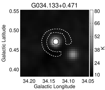
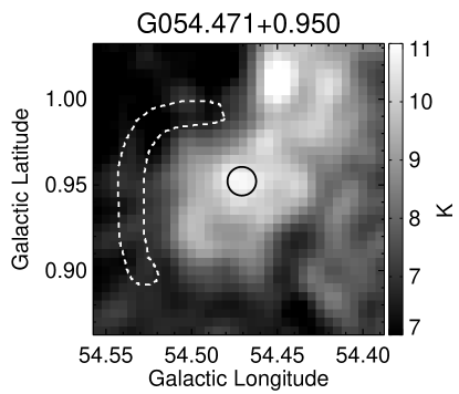
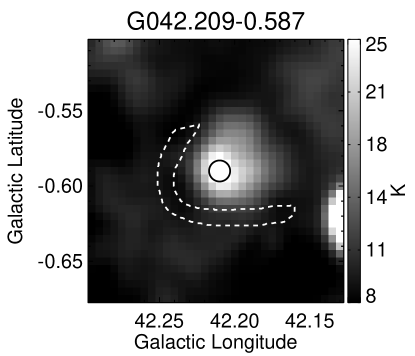
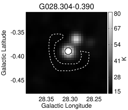
Figure 1: On– and off–source apertures for two H II regions. The on–source apertures are shown with solid lines and the off–source apertures with dashed lines. The background images are VGPS 21 cm continuum data.

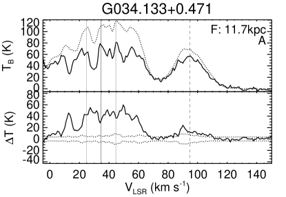
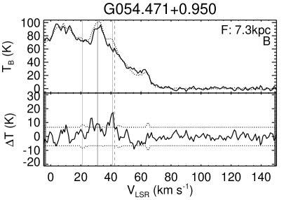
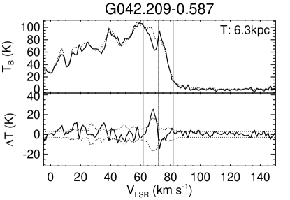
Figure 2: Example difference spectra for the same HRDS sources shown in Figure 1. The top panel of each plot shows the on– (solid line) and off– (dotted line) source average H I spectra. The bottom panel of each plot shows the difference between the off– and on–source spectra (solid line) and our error estimates (dotted lines; see §3). The three solid vertical lines mark the RRL velocity and $\pm$10 $\,{\rm km\,s^{-1}}$ of the RRL velocity, and the dashed vertical line marks the tangent point velocity. We assigned each source a qualitative quality factor (QF) of “A,” “B,” or “C” (see text). Clockwise from top-left are a far source of QF A, a far source of QF B, a near source of QF A, and a tangent point source (where no KDA resolution would be possible based on the difference spectrum, and no QF is assigned). In the top right corner of each plot we give the KDA resolution (“N,”, “F,”, or “T” for near, far, or tangent point), followed by the assigned distance in kpc. Below this we print the QF.

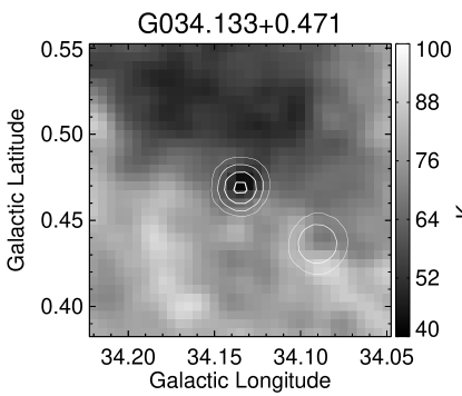
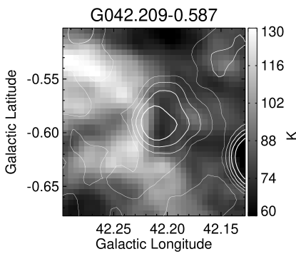
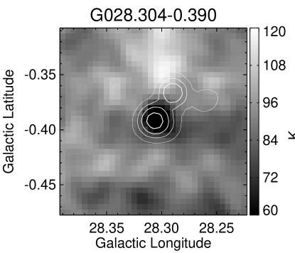
Figure 3: Example H I channel maps at the velocity of maximum absorption for the same sources shown in Figure 1. The contours are 21 cm VGPS continuum emission. The H II regions are at the center of their respective panels. The morphological agreement between the H I absorption and the radio continuum emission demonstrates that the absorption signals are likely real (although the situation is slightly ambiguous for G042.209$-$0.587, which is located at the tangent point).

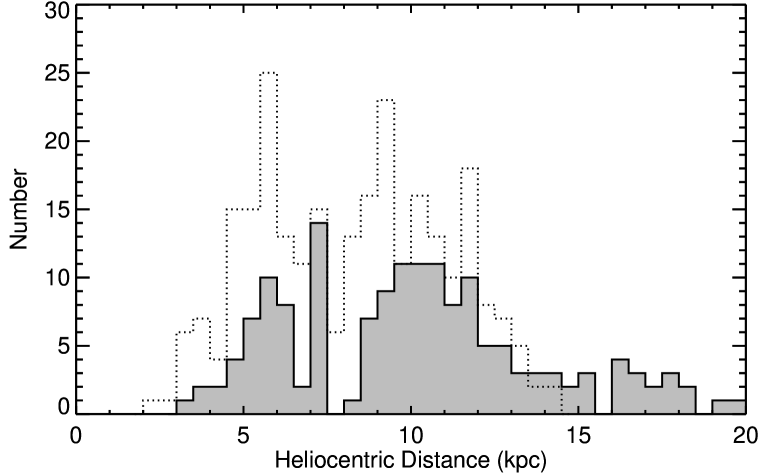
Figure 4: Distribution of Heliocentric distances HRDS (gray filled) and the AB sample (dotted line). The HRDS nebulae are on average more distant, and in fact the two samples are statistically distinct.

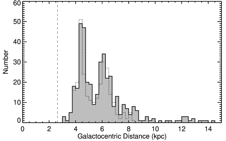
Figure 5: Distribution of Galactocentric radii for the HRDS (gray filled) and the AB sample (dotted line). The two samples are statistically similar. The vertical dashed line shows the minimum Galactocentric radius sampled by the present study. The peaks at 4.25 and 6.0 kpc are only about 1 kpc wide, for both samples.

Figure 6: Galactic distribution of H II regions. The Sun is located in the upper left corner and the Galactic center is at (0, 0). The plot contains both HRDS sources (triangles) and also H II regions known prior to the HRDS from AB (crosses). The straight solid lines show the longitude range of the present study, $17\fdg 9$ to $67\arcdeg$ (the longitude range of AB is different). The solid half-circle shows the tangent-point distance and the dotted half circle shows the Solar orbit. The left panel shows the positions for all regions with assigned distances. In the right panel, we binned these positions into $0.15\times 0.15$ $\,{\rm kpc}$ pixels, and smoothed the resultant image with a $5\times 5$ pixel Gaussian filter. The semicircular arc-segments correspond to the peaks in the Galactocentric radius distribution seen in Figure 5.

Figure 7: The total uncertainties associated with the choice of rotation curve, the effect of non-circular motions, and changing the Solar rotation speed for near distances (left panel) and far distances (right panel). We mark the example position mentioned in the text, $(\ell,v)$ $=(50\,^{\circ},30\,\,{\rm km\,s^{-1}})$, with an “x”.

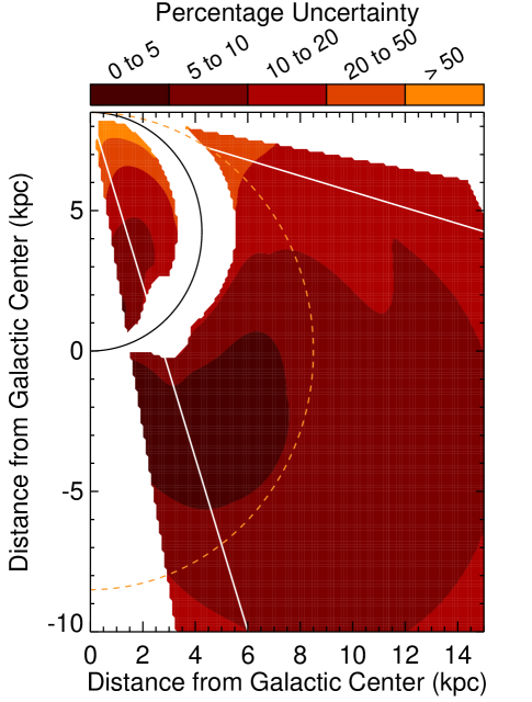
Figure 8: Face-on map of the total percentage uncertainty in kinematic distances caused by the choice of rotation curve, non-circular motions of 7 $\,{\rm km\,s^{-1}}$, and by changing the Solar circular rotation speed to 250 $\,{\rm km\,s^{-1}}$. The meaning of the curves and lines are as in Figure 12.

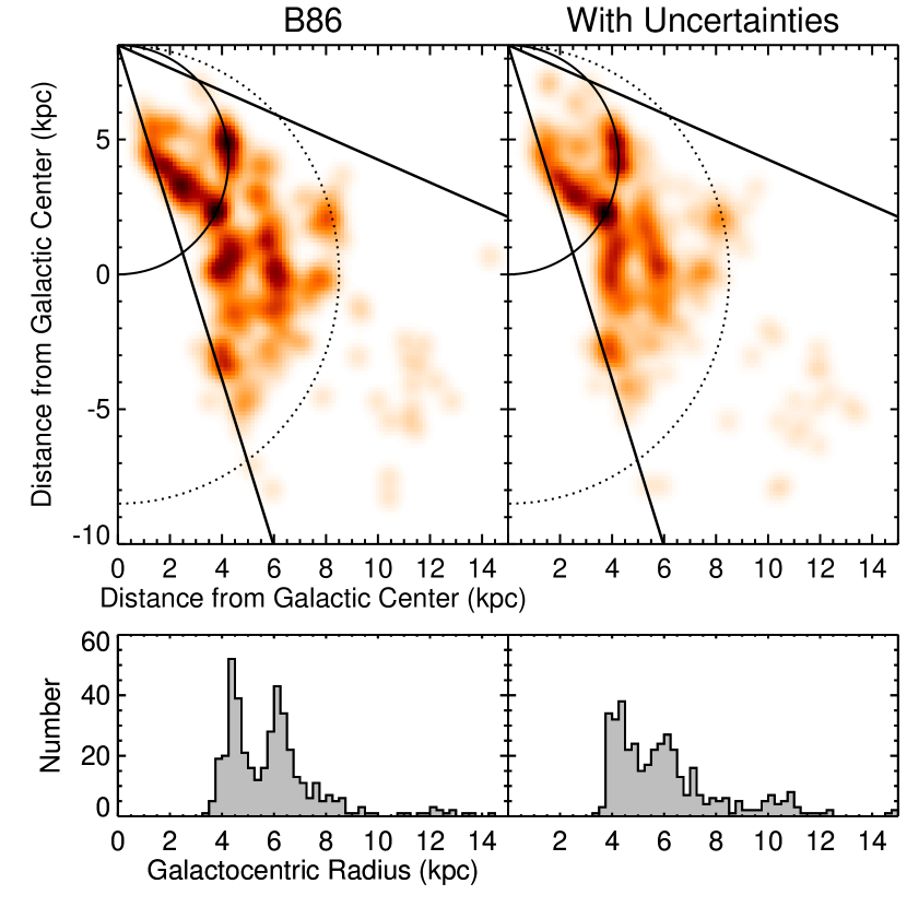
Figure 9: The effect of distance uncertainties on Figures 5 and 6. In the top row we show the smoothed face-on plot of the HRDS and previously known H II regions; in the top left panel we calculate the distances using the B86 curve and in the top right panel we have accounted for uncertainties caused by the choice of rotation curve, non-circular motions, and a change to the Solar circular rotation speed. The lines in the top panels are as in Figures 6. The bottom row shows the distribution of Galactocentric radii for the B86 curve (bottom left panel), and after accounting for these sources of distance uncertainty (bottom right panel), for the same sources shown in the top row. The basic structures are largely unchanged.

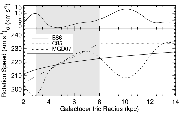
Figure 10: The circular rotation speed versus Galactocentric radius for the B86 curve (solid line), the C85 curve (dashed line), and the MGD07 curve (dotted line). In the upper panel, we show the standard deviation between the three curves. The shaded region shows the range of Galactocentric radii over which the MGD07 curve is defined, 3–8 kpc. We extrapolate the MGD07 curve below 3 kpc and assume a flat rotation curve above 8 kpc.

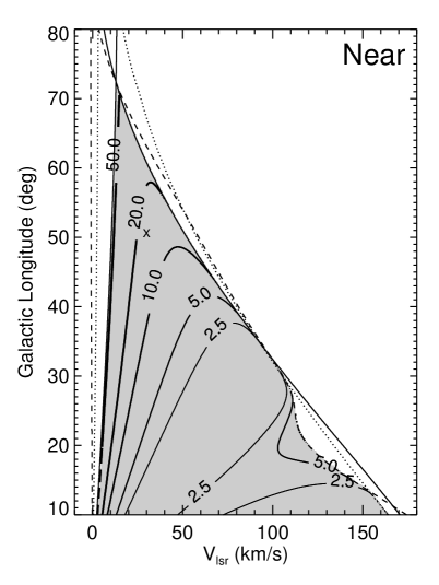
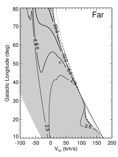
Figure 11: The percentage uncertainty in kinematic distances associated with the choice of rotation curve. Each $(\ell,v)$ locus gives the standard deviation in the distances computed using the C85, B86, and MGD07 rotation curves divided by the distance calculated using the B86 rotation curve. We mark the example position mentioned in the text, $(\ell,v)$ $=(50\,^{\circ},30\,\,{\rm km\,s^{-1}})$, with an “x”. The left panel shows the percentage uncertainty in near distances and the right panel shows the same for far distances. The gray area contains $(\ell,v)$ locii that are defined for all three rotation curves whereas white areas are undefined for one or more rotation curves. The three curved lines (not including the contours) show the $(\ell,v)$ locii where the near distance is zero, and also the $(\ell,v)$ locii of the tangent point for the B86 curve (solid), C85 curve (dashed), and the MGD07 curve (dotted).

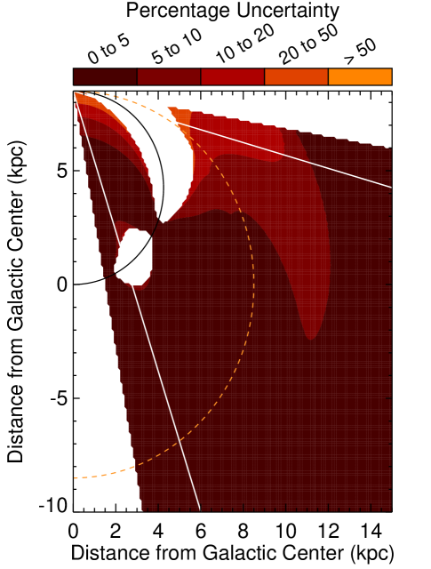
Figure 12: Face-on map of the percentage uncertainty in the three rotation curve models. The tangent point distance is shown as the solid curve and the Solar orbit is shown as the dashed curve. The range of the HRDS sources with assigned distances is shown with straight lines. The white holes in the figure shows areas that are not defined for all three rotation curves.

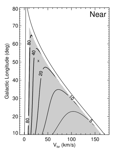
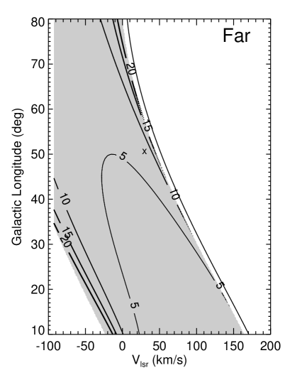
Figure 13: The percentage uncertainty in kinematic distances associated with non-circular motions of $7\,\,{\rm km\,s^{-1}}$ for near (left panel) and far distances (right panel). The solid black lines show the $(\ell,v)$ locii where the near distance is zero, and also the $(\ell,v)$ locii of the tangent point for the B86 curve. We mark the example position mentioned in the text, $(\ell,v)$ $=(50\,^{\circ},30\,\,{\rm km\,s^{-1}})$, with an “x”.

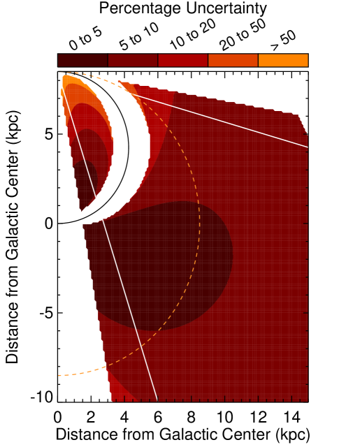
Figure 14: Face-on map of the percentage uncertainty in kinematic distances associated with non-circular motions of 7 $\,{\rm km\,s^{-1}}$. The meaning of the curves and lines are the same as in Figure 12. No comparison may be made within 7 $\,{\rm km\,s^{-1}}$ of the tangent point velocity, which leads to the white area surrounding the tangent point distance where no uncertainties are calculated.

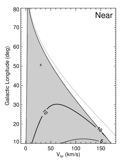
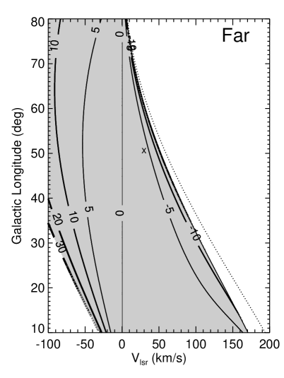
Figure 15: The percentage uncertainty associated with changing the circular Solar rotation speed from 220 $\,{\rm km\,s^{-1}}$ to 250 $\,{\rm km\,s^{-1}}$ for near (left panel) and far distances (right panel). The black lines show the $(\ell,v)$ locii where the near distance is zero, and also the $(\ell,v)$ locii of the tangent point for the B86 curve with $\Theta_{0}=220\,\,{\rm km\,s^{-1}}$. The dotted line shows the same for $\Theta_{0}=250\,\,{\rm km\,s^{-1}}$. We mark the example position mentioned in the text, $(\ell,v)$ $=(50\,^{\circ},30\,\,{\rm km\,s^{-1}})$, with an “x”.

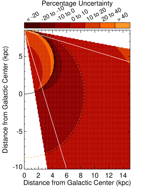
Figure 16: Face-on map of the percentage uncertainty caused by changing the Solar rotation speed to 250 $\,{\rm km\,s^{-1}}$. The meaning of the curves and lines are as in Figure 12.

References

- Anderson & Bania (2009) Anderson, L. D., & Bania, T. M. 2009, ApJ, 690, 706
- Anderson et al. (2011) Anderson, L. D., Bania, T. M., Balser, D. S., & Rood, R. T. 2011, ApJS, 194, 32 (Paper II)
- Araya et al. (2002) Araya, E., Hofner, P., Churchwell, E., & Kurtz, S. 2002, ApJS, 138, 63
- Balser et al. (2011) Balser, D. S., Rood, R. T., Bania, T. M., & Anderson, L. D. 2011, ApJ, 738, 27
- Bania et al. (2010) Bania, T. M., Anderson, L. D., Balser, D. S., & Rood, R. T. 2010, ApJ, 718, L106 (Paper I)
- Bania & Lockman (1984) Bania, T. M., & Lockman, F. J. 1984, ApJS, 54, 513
- Benjamin et al. (2005) Benjamin, R. A., et al. 2005, ApJ, 630, L149
- Blitz et al. (1982) Blitz, L., Fich, M., & Stark, A. A. 1982, ApJS, 49, 183
- Brand (1986) Brand, J. 1986, PhD thesis, Leiden Univ., Netherlands.
- Brand et al. (1987) Brand, J., Blitz, L., Wouterloot, J. G. A., & Kerr, F. J. 1987, A&AS, 68, 1
- Brand & Wouterloot (1988) Brand, J., & Wouterloot, J. G. A. 1988, A&AS, 75, 117
- Burton (1966) Burton, W. B. 1966, Bull. Astron. Inst. Netherlands, 18, 247
- Burton & Gordon (1976) Burton, W. B., & Gordon, M. A. 1976, ApJ, 207, L189
- Burton & Gordon (1978) —. 1978, A&A, 63, 7
- Churchwell et al. (2006) Churchwell, E., et al. 2006, ApJ, 649, 759
- Clemens (1985) Clemens, D. P. 1985, ApJ, 295, 422
- Downes et al. (1980) Downes, D., Wilson, T. L., Bieging, J., & Wink, J. 1980, A&AS, 40, 379
- Fich et al. (1989) Fich, M., Blitz, L., & Stark, A. A. 1989, ApJ, 342, 272
- Gibson et al. (2005) Gibson, S. J., Taylor, A. R., Higgs, L. A., Brunt, C. M., & Dewdney, P. E. 2005, ApJ, 626, 195
- Gómez (2006) Gómez, G. C. 2006, AJ, 132, 2376
- Jackson et al. (2002) Jackson, J. M., Bania, T. M., Simon, R., Kolpak, M., Clemens, D. P., & Heyer, M. 2002, ApJ, 566, L81
- Jackson et al. (2006) Jackson, J. M., et al. 2006, ApJS, 163, 145
- Knapp (1974) Knapp, G. R. 1974, AJ, 79, 527
- Kolpak et al. (2003) Kolpak, M. A., Jackson, J. M., Bania, T. M., Clemens, D. P., & Dickey, J. M. 2003, ApJ, 582, 756
- Kuchar & Bania (1994) Kuchar, T. A., & Bania, T. M. 1994, ApJ, 436, 117
- Levine et al. (2008) Levine, E. S., Heiles, C., & Blitz, L. 2008, ApJ, 679, 1288
- Liszt et al. (1981) Liszt, H. S., Burton, W. B., & Bania, T. M. 1981, ApJ, 246, 74
- Lockman (1979) Lockman, F. J. 1979, ApJ, 232, 761
- Lockman (1981) —. 1981, ApJ, 245, 459
- Lockman (1989) —. 1989, ApJS, 71, 469
- McClure-Griffiths & Dickey (2007) McClure-Griffiths, N. M., & Dickey, J. M. 2007, ApJ, 671, 427
- McClure-Griffiths et al. (2005) McClure-Griffiths, N. M., Dickey, J. M., Gaensler, B. M., Green, A. J., Haverkorn, M., & Strasser, S. 2005, ApJS, 158, 178
- Mezger (1970) Mezger, P. G. 1970, in IAU Symposium, Vol. 38, The Spiral Structure of our Galaxy, ed. W. Becker & G. I. Kontopoulos, 107
- Payne et al. (1980) Payne, H. E., Terzian, Y., & Salpeter, E. E. 1980, ApJ, 240, 499
- Radhakrishnan & Goss (1972) Radhakrishnan, V., & Goss, W. M. 1972, ApJS, 24, 161
- Rathborne et al. (2009) Rathborne, J. M., Johnson, A. M., Jackson, J. M., Shah, R. Y., & Simon, R. 2009, ApJS, 182, 131
- Reid et al. (2009) Reid, M. J., et al. 2009, ApJ, 700, 137
- Roman-Duval et al. (2010) Roman-Duval, J., Jackson, J. M., Heyer, M., Rathborne, J., & Simon, R. 2010, ApJ, 723, 492
- Russeil et al. (2007) Russeil, D., Adami, C., & Georgelin, Y. M. 2007, A&A, 470, 161
- Sanders et al. (1986) Sanders, D. B., Clemens, D. P., Scoville, N. Z., & Solomon, P. M. 1986, ApJS, 60, 1
- Sanna et al. (2009) Sanna, A., Reid, M. J., Moscadelli, L., Dame, T. M., Menten, K. M., Brunthaler, A., Zheng, X. W., & Xu, Y. 2009, ApJ, 706, 464
- Schlingman et al. (2011) Schlingman, W. M., et al. 2011, ApJS, 195, 14
- Sewilo et al. (2004) Sewilo, M., Churchwell, E., Kurtz, S., Goss, W. M., & Hofner, P. 2004, ApJ, 605, 285
- Sharpless (1953) Sharpless, S. 1953, ApJ, 118, 362
- Stil et al. (2006) Stil, J. M., et al. 2006, AJ, 132, 1158
- Urquhart et al. (2012) Urquhart, J. S., et al. 2012, MNRAS, 420, 1656
- Watson et al. (2003) Watson, C., Araya, E., Sewilo, M., Churchwell, E., Hofner, P., & Kurtz, S. 2003, ApJ, 587, 714
- Wilson (1972) Wilson, T. L. 1972, A&A, 19, 354