Impact cratering on Mercury: consequences for the spin evolution

Abstract

Impact basins identified by Mariner 10 and Messenger flyby images provide us a fossilized record of the impactor flux of asteroids on Mercury during the last stages of the early Solar System. The distribution of these basins is not uniform across the surface, and is consistent with a primordial synchronous rotation (Wieczorek et al., 2012). By analyzing the size of the impacts, we derive a simple collisional model coherent with the observations. When combining it with the secular evolution of the spin of Mercury, we are able to reproduce the present 3/2 spin-orbit resonance ($\sim$50% of chances), as well as a primordial synchronous rotation. This result is robust with respect to variations in the dissipation and collisional models, or in the initial spin state of the planet.

1. Introduction

Mercury is known to be in a 3/2 spin-orbit resonance (Pettengill & Dyce, 1965; Colombo, 1965; Goldreich & Peale, 1966). However, recent investigation on the locations of ancient impact basins on Mercury (pre-Caloris basin) has shown that they are not uniformly distributed across the surface, and that their distribution is consistent with the spatial variations that would arise if Mercury were once in a state of synchronous rotation (Wieczorek et al., 2012). Assuming an initial prograde rotation for Mercury, the 3/2 resonance arises naturally, but the synchronous rotations is almost impossible to achieve ($<4$% of chances) due to the high values of Mercury’s orbital eccentricity (Correia & Laskar, 2004, 2009). An alternate scenario for capture into the 1/1 resonance is to suppose that Mercury’s initial spin was retrograde, since planetary accretion models seem to allow terrestrial planets to have either prograde or retrograde initial spin rates (Dones & Tremaine, 1993; Kokubo & Ida, 2007). In this case, synchronous rotation becomes the most likely outcome, but a subsequent evolution into the presently observed 3/2 resonant rotation requires a large impact event (Wieczorek et al., 2012).

In the present Letter, we extend further the dynamical analysis of asteroid impacts on the planet surface. We obtain the impactor flux on Mercury from the present crater distribution (Sect. 2), and provide two simple models for collisions (Sect. 3). Then, using a secular spin evolution model for Mercury (Sect. 4) with collisions, we determine the chances of capture in each spin-orbit resonance (Sect. 5), and derive our conclusions (Sect. 6).

2. Impact cratering

Cratering is one of the most important geological processes that shape and modify the surfaces of terrestrial planets and satellites. The quantification of the impactor source population on Mercury and the observation of its surface help to understand the dynamical history of both the impactor population and the spin of the planet.

Impact basins identified by Mariner 10 based geological mapping (Spudis & Guest, 1988) and Messenger flyby images (Fassett et al., 2011; Herrick et al., 2011) provide us a fossilized record of the impactor flux of asteroids during the last stages of the early Solar System. The spatial density of craters smaller than 100 km in diameter have been affected by more recent geologic processes and the numerous craters that are somewhat larger than this might also be in saturation (Fassett et al., 2011). In addition, the minimal crater size to escape the presently observed 3/2 spin-orbit resonance is estimated to be 300 km (Wieczorek et al., 2012). Therefore, here we restrict our analysis to those basins that are larger than 300 km (Table 1).

Table 1Impact basins on Mercury with diameters greater than 300 km (Wieczorek et al., 2012).

Crater	Lat.	Long.	$D_{\mathrm{basin}}$	$D$
(name)	(∘N)	(∘E)	(km)	(km)
Caloris	$+30.9$	$+159.7$	1456.7	188.9
Andal-Coleridge	$-43.0$	$-49.0$	1300.0	163.8
Tir	$+6.0$	$-168.0$	1250.0	156.0
Eitoku-Milton	$-23.0$	$-171.0$	1180.0	145.2
Bartok-Ives	$-33.0$	$-115.0$	1175.0	144.4
Donne-Moliere	$+4.0$	$-10.0$	1060.0	126.9
Sadi-Scopas	$-83.0$	$-44,0$	930.0	107.8
Budh	$-17.0$	$-151.0$	850.0	96.3
Matisse-Repin	$-23.4$	$-75.2$	843.2	95.4
Mena-Theophanes	$-2.3$	$-126.7$	836.1	94.4
Sobkou	$+33.4$	$-133.5$	785.3	87.3
Borealis	$+72.1$	$-80.9$	785.2	87.2
Rembrandt	$-33.1$	$+87.7$	696.7	75.1
Vincente-Yakovlev	$-52.6$	$-162.1$	692.5	74.6
Ibsen-Petrarch	$-31.0$	$-30.0$	640.0	67.6
Beethoven	$-20.8$	$-123.9$	632.5	66.6
Brahams-Zola	$+59.0$	$-172.0$	620.0	64.9
(unnamed)	$+4.7$	$+74.1$	529.6	53.3
Tolstoj	$-17.1$	$-164.6$	500.6	49.7
Hawthorne-Riemen.	$-56.0$	$-105.0$	500.0	49.6
Gluck-Holbein	$+35.0$	$-19.0$	500.0	49.6
(unnamed)	$+0.6$	$+93.4$	428.4	40.9
(unnamed)	$-39.0$	$-101.4$	420.3	39.9
Dostoevskij	$-44.8$	$-177.1$	413.9	39.2
(unnamed)	$-44.5$	$-93.2$	411.4	38.9
Derzhavin-Sor Juana	$+50.8$	$-26.9$	406.3	38.3
(unnamed)	$-2.6$	$-56.1$	392.6	36.7
(unnamed)	$+27.9$	$-158.6$	389.0	36.3
Vyasa	$+50.7$	$-85.1$	379.9	35.2
Shakespeare	$+48.9$	$-152.3$	357.2	32.6
Hiroshige-Mahler	$-17.0$	$-23.0$	340.3	30.7
Chong-Gauguin	$+57.1$	$-107.9$	325.6	29.0
Raphael	$-20.3$	$-76.1$	320.4	28.5
Goethe	$+81.5$	$-54.3$	319.0	28.3
(unnamed)	$-2.5$	$-44.6$	311.4	27.5
(unnamed)	$+28,9$	$-113.8$	307.9	27.1
(unnamed)	$-25.0$	$-98.8$	307.6	27.0
(unnamed)	$-17.3$	$-96.8$	$303.4$	26.6

Cratering processes have been extensively studied through impact and explosion experiments (e.g. Schmidt & Housen, 1987). By interpreting the observations of the Deep Impact event, Holsapple & Housen (2007) derived an expression that allow us to estimate the diameter of a basin, $D_{\mathrm{basin}}$, as a function of the diameter of the impactor, $D$. For non porous rocks, we have (Le Feuvre & Wieczorek, 2011):

$$D_{\mathrm{basin}}\approx 1.92\,D\left(\frac{u^{2}}{gD}\right)^{0.22}\left(\frac{\rho_{a}}{\rho}\right)^{0.31}\ ,$$ (1)

where $\rho$ and $\rho_{a}$ are respectively the densities of the planet and the impactor, $g$ is the surface gravity of the planet, and $u$ the normal impact velocity component. Adopting Mercury’s values for $\rho$ and $g$, a mean density for the asteroids $\rho_{a}=2.5$ g/cm³ (Fienga et al., 2011), and an average speed of $u=42.5$ km/s (Le Feuvre & Wieczorek, 2008), we can estimate the size of the bodies that opened the basins currently observed (Table 1):

$${D}_{\mathrm{[km]}}\approx\left(\frac{{D_{\mathrm{basin}}}_{\mathrm{[km]}}}{22}\right)^{1.25}\ .$$ (2)

We can now derive the cumulative distribution of the impact number on Mercury as a function of the size of the bodies. In Figure 1 we used bins of 5 km and each dot gives the position of the bin. This distribution provides a reliable estimation of the impactor flux during the late heavy bombardment some 3.8 Gyr ago (Kring & Cohen, 2002). We simultaneously plot the present size distribution in the asteroid-belt (e.g. Jedicke et al., 2002), normalized by a factor 50, such that the number of largest bodies coincide with the observed number of impacts on Mercury. Although the two populations distributions are quite similar for $D_{\mathrm{crit}}>110$ km, for smaller diameters it appears that the number of impacts is clearly smaller.

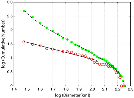
Figure 1.— Cumulative number of impacts observed on Mercury’s surface (IMD, red), and normalized size distribution in the asteroid-belt (ABD, green). The diameter of the bodies is binned in classes of 5 km.

3. Collisional models

A realistic long-term evolution of the spin of Mercury can only be complete if one takes into account the effect from collisions during the early stages of its evolution. Escape from spin-orbit resonances can occur by variations in the eccentricity (Correia & Laskar, 2004, 2009), but evolution beyond these states is also possible through the momentum imparted to the planet during a basin-forming impact event (e.g. Melosh, 1975). In particular, the synchronous resonance can only be unlocked by this method (Lissauer, 1985; Wieczorek & Le Feuvre, 2009).

The presently observed craters on the planet’s surface provide us important information on the size and distribution of the impacts, but few on their consequences to the spin of the planet. Therefore, we adopt here a simple model to take into account large impacts on Mercury, that uses either the observed crater or asteroid distributions to generate similar random impacts.

We assume that the impact probability is uniformly distributed over the whole surface of the planet. The rotational angular momentum of Mercury prior to the collision is given by $\mathbf{L}_{0}=C\omega_{0}\mathbf{k}_{0}$, where $C$ is the principal moment of inertia, $\omega$ the rotation rate, and $\mathbf{k}$ a unit-vector along the spin axis. The impactor has mass $m_{i}$ and hits the planet at a point of the surface given by $\mathbf{R}$.The planet has mass $m$, and assuming $m_{i}\ll m$ the angular momentum change is simply obtained by

$$\mathbf{L}=C\omega\mathbf{k}=C\omega_{0}\mathbf{k}_{0}+m_{i}\mathbf{R}\times\mathbf{u}\ ,$$ (3)

where $\mathbf{u}$ is the differential velocity between Mercury and the impactor.

We assume also for simplicity that the orbit of Mercury is circular $(r=a)$ and coplanar with the orbit of the impactor. Whenever the position of the impactor $\mathbf{r}_{i}$ crosses the orbit of Mercury, a collision can occur, that is, when $r_{i}=a$. Thus, we compute the relative velocity as

$$u=na\sqrt{3-\frac{a}{a_{i}}-2\sqrt{\frac{a_{i}}{a}(1-e_{i}^{2})}}\ ,$$ (4)

where $a$ is the semimajor axis, $e$ the eccentricity, and $n$ the mean motion. Based on the present distribution of Mercury-crossing objects, we assume that the impactor has origin in the asteroid belt, thus $a_{i}=a_{A}/(1+e_{i})$, and $e_{i}\geq(a_{A}-a)/(a_{A}+a)$, where $a_{A}\approx 2.5$ AU.

Finally, we assume that the initial obliquity of the planet is zero, i.e., $\mathbf{k}_{0}$ is normal to the orbital plane. Using for simplicity the reference frame $(\mathbf{i}_{0},\mathbf{j}_{0},\mathbf{k}_{0})$ linked to the orbital plane of Mercury, where $\mathbf{j}_{0}$ is along the direction of $\mathbf{u}$, we have

$$\mathbf{R}\times\mathbf{u}=-R_{a}u\sin\phi\,\mathbf{i}_{0}+R_{a}u\cos\phi\,\mathbf{k}_{0}\ ,$$ (5)

where $R_{a}=||\mathbf{R}\times\mathbf{u}||/u$ is the moment arm, which is perpendicular to $\mathbf{u}$, and $\phi$ is the angle between $\mathbf{i}_{0}$ and the impact point direction. Using expression (3), the change in the rotation rate after impact is

$$\left(\frac{\omega}{\omega_{0}}\right)^{2}=1+\ell^{2}+2\ell\cos\phi\ ,$$ (6)

where $\ell=m_{i}R_{a}u/(C\omega_{0})$. In Table 2 we list the minimal impactor diameter needed to disrupt each spin-orbit resonance for different eccentricities ($R_{a}=R$ and $\phi=0^{\circ}$) with an average speed of $u=42.5$ km/s (Le Feuvre & Wieczorek, 2008).

Table 2Critical eccentricity and minimal impactor diameter needed to destabilize each spin-orbit resonance.

$p$	$e_{\mathrm{crit.}}$	$D$ (km)
		$e=0.1$	$e=0.2$	$e=0.3$
5/1	0.211334	$-$	$-$	20.4
9/2	0.174269	$-$	14.9	23.0
4/1	0.135506	$-$	17.9	26.2
7/2	0.095959	12.2	21.4	29.4
3/1	0.057675	16.3	25.5	32.7
5/2	0.024877	21.5	30.0	36.0
2/1	0.004602	27.9	34.8	39.1
3/2	0.000026	35.4	39.3	41.2
1/1	$-$	40.6	41.6	42.1
1/2	0.000180	25.7	28.8	30.8

The quantities $(m_{i},e_{i})$ depend on the impactor and $(R_{a},\phi)$ on the impact point. They are the only variables unknown in the model and they need to be randomized in order to simulate the collisions.

We assumed that impacts over the surface of Mercury are uniformly distributed. Thus, the probability density function (PDF) for $\phi$ is constant in the interval $[0,2\pi]$, while for the moment arm $R_{a}$ the PDF is linear in the interval $[0,R]$ (Laskar et al., 2011). If $x$ is a random variable uniform in the interval $[0,1]$ we then compute:

$$\phi=2\pi x\ ,\quad R_{a}=R\sqrt{x}\ .$$ (7)

For the periastron of the impactor $p_{i}=a_{A}(1-e_{i})/(1+e_{i})$, we use a similar distribution as for $R_{a}$, that is, we assume that the PDF for $p_{i}$ is linear in the interval $[0,a]$:

$$p_{i}=a\sqrt{x}\quad\Rightarrow\quad e_{i}=\frac{a_{A}-a\sqrt{x}}{a_{A}+a\sqrt{x}}\ .$$ (8)

Finally, for the mass distribution we use either the present asteroid-belt distribution (ABD), or the observed impacts on Mercury distribution (IMD). The total number of collisions $N$ is a parameter that can be adjusted in the model, and the corresponding distribution of the masses is given by $m_{i}=\pi\rho_{a}D^{3}/6$.

The ABD can be fitted by a polynomial curve of degree three (dashed line, Fig. 1):

$$\log D=0.06\,y^{3}-0.28\,y^{2}+0.03\,y+2.25\ ,$$ (9)

where $y=\log(xN)$.

The IMD appears to have a bump near $D_{\mathrm{crit}}\sim 110$ km, that can be explained by different collisional regimes in the asteroid-belt (e.g. Bottke et al., 2005). We fitted an incremental power-law to the two different regions and obtained an index of $-1.2$ for sizes $D_{\mathrm{crit}}<110$ km (solid line, Fig. 1), and $-4.5$ for $D_{\mathrm{crit}}>110$ km. The cumulative distribution functions is then given by

$$P_{cum.}=\left\{\begin{array}[]{l c r}\left(\frac{D_{0}}{D}\right)^{1.2}&\mathrm{if}&D_{0}\leq D\leq D_{\mathrm{crit}}\ ,\cr\vskip 6.0pt plus 2.0pt minus 2.0pt\cr\left(\frac{D_{1}}{D}\right)^{4.5}&\mathrm{if}&D_{\mathrm{crit}}<D\leq 200\mathrm{~{}km}\ ,\end{array}\right.$$ (10)

with

$$D_{0}=\left(\frac{40}{N}\right)^{\frac{1}{1.2}}\times\mathrm{30~{}km}\quad\mathrm{and}\quad D_{1}=\left(\frac{D_{0}}{D_{\mathrm{crit}}}\right)^{\frac{1.2}{4.5}}\times D_{\mathrm{crit}}\ ,$$ (11)

where $D_{\mathrm{crit}}=110$ km, and 30 km is the approximate size of a body needed to open a 300 km diameter crater on Mercury (Eq. 2). Thus,

$$D=\left\{\begin{array}[]{l c r}D_{1}\,x^{-\frac{1}{4.5}}&\mathrm{if}&x\in[0,x_{0}[\ ,\cr\vskip 6.0pt plus 2.0pt minus 2.0pt\cr D_{0}\,x^{-\frac{1}{1.2}}&\mathrm{if}&x\in[x_{0},1]\ ,\end{array}\right.$$ (12)

where $x_{0}=(D_{0}/D_{1})^{\frac{5.4}{3.3}}$.

In our simulations we set $N=100$, which gives $\log(xN)=\log x+2$, $D_{0}\approx 14$ km, $D_{1}\approx 64$ km, and $x_{0}\approx 8.4\times 10^{-2}$. For both ABD and IMD, if $D>200$ km we repeat the interaction given by expressions (9) and (12), respectively.

Table 3Capture probabilities in several spin-orbit resonances (in percentage).

$p$	previous studies				IMD		ABD
	GP66	CL04	CL09	Wi12	prograde	retrograde	prograde	retrograde
4/1	$-$	$-$	$-$	$-$	$-$	$-$	$-$	$-$
7/2	0.1	$-$	4.7	$-$	$-$	$-$	$-$	$-$
3/1	0.4	$-$	11.6	$-$	$-$	0.1	$-$	0.2
5/2	1.4	$-$	22.1	0.1	0.3	$-$	0.2	0.2
2/1	1.7	3.6	31.6	0.4	3.7	2.5	2.9	2.7
3/2	7.2	55.4	25.9	2.4	49.4	52.2	50.6	50.1
1/1	$-$	2.2	3.9	68.2	26.9	25.9	24.2	25.1
1/2	$-$	$-$	$-$	28.9	0.1	$-$	$-$	$-$
none	89.2	38.3	0.2	$-$	19.6	19.3	22.1	21.7

4. Spin dynamics model

Tidal dissipation and core-mantle friction drive the obliquity of Mercury close to $0^{\circ}$ or $180^{\circ}$ (Correia & Laskar, 2010). For zero degree obliquity, and in absence of dissipation, the averaged equation for the rotational motion near the $p$ resonance (where $p$ is a half-integer) writes (Goldreich & Peale, 1966; Correia, 2006):

$$\dot{\omega}=-\frac{3}{2}n^{2}\frac{B-A}{C}H(p,e)\sin 2(\theta-pM)\ ,$$ (13)

where $M$ is the mean anomaly, $\omega=\dot{\theta}$, $H(p,e)$ are Hansen coefficients, and $A<B<C$ are the moments of inertia.

For tidal dissipation we adopt a linear viscous model (e.g. Mignard, 1979) in agreement with a Maxwell rheology for slow rotations. Its contribution to the rotation rate is given by (e.g. Correia, 2009):

$$\dot{\omega}=-K\left[\Omega(e)\omega-N(e)n\right]\ ,$$ (14)

with

$$\Omega(e)=\frac{1+3e^{2}+3e^{4}/8}{(1-e^{2})^{9/2}}\ ,$$ (15)

$$N(e)=\frac{1+15e^{2}/2+45e^{4}/8+5e^{6}/16}{(1-e^{2})^{6}}\ ,$$ (16)

and

$$K=3n\frac{k_{2}}{\xi\,Q}\left(\frac{R}{a}\right)^{3}\left(\frac{m_{\odot}}{m}\right)\ ,$$ (17)

where $m_{\odot}$ is the solar mass, $k_{2}$ is the second Love number, $Q$ the quality factor, and $\xi=C/mR^{2}$.

The Mariner 10 flyby of Mercury and subsequent observations made with Earth-based radar provided strong evidence of a conducting existent fluid core (Ness, 1978; Margot et al., 2007). The resulting core-mantle friction (CMF) may be expressed by an effective torque (Goldreich & Peale, 1967; Correia & Laskar, 2010):

$$\dot{\omega}=-c_{c}\kappa(\omega-\omega_{c})\quad\mathrm{and}\quad\dot{\omega}_{c}=c_{m}\kappa(\omega-\omega_{c})\ ,$$ (18)

where $\kappa$ is an effective coupling parameter, $\omega_{c}$ the core’s rotation rate, and $c_{c}=C_{c}/C=1-c_{m}=0.45$ (Margot et al., 2007). We also have $\kappa=2.62\sqrt{\nu\omega}/(c_{m}R_{c})$ (Mathews & Guo, 2005), where $R_{c}$ is the core radius and $\nu$ is the kinematic effective viscosity of the core.

When considering the perturbations of the other planets, the eccentricity of Mercury undergoes strong chaotic variations in time (Laskar, 1994, 2008; Correia & Laskar, 2004, 2009). These variations are modeled using the averaging of the equations for the motion of the Solar System, that have been compared to numerical integrations, with very good agreement (Laskar et al., 2004a, b). The mean value of the eccentricity is $0.198$, slightly lower than the present value, but we also observe a wide range for the eccentricity variations, from nearly zero to more than 0.45. Even if some of these episodes do not last for a long time, they will allow additional capture into and escape from spin-orbit resonances (Table 2 and 3).

5. Numerical simulations

Assuming an initial rotation period of Mercury of 8 h, we estimated the time needed to despin the planet to the slow rotations to about 300 million years. This motivates that our starting time is $-4$ Gyr, although this value is not critical. Due to the chaotic behavior of the eccentricity (Laskar, 1989, 1990), we have performed a statistical study of the past evolutions of Mercury’s orbit, with the integration of 1000 orbits in the past, starting with very close initial conditions, within the uncertainty of the present ones. For each of these 1000 orbital solutions, we have integrated numerically the rotation motion of Mercury, taking into account the resonant terms (Eq.13), for $p=k/2;k=-14,\dots,14$, the tidal dissipation (Eq.14), the CMF (Eq.18), and the planetary perturbations. We adopted for all model parameters the same values as in Correia & Laskar (2009). The effect from the collisions (Sect. 3) is only considered between $-4.0$ and $-3.8$ Gyr in the past.

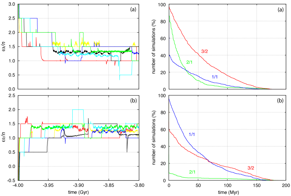
Figure 2.— Left: Some examples of Mercury’s rotation rate evolution during the collisional period. Right: Cumulative time spent in each spin-orbit resonance (IMD). (a) For initial prograde rotation. (b) For initial retrograde rotation.

In a first experiment, we use the IMD for collisions, and the initial rotation period of Mercury is set at 10 day (prograde rotation). As in previous studies, the spin encounters higher order resonances first, and capture often occurs (Fig. 2a). Small impacts cause the planet to librate in longitude about the resonance center, with the amplitude damping with time, but for sufficiently large impacts, escape from all resonances may occur (Tab. 2). Half of these breaking events increase the rotation rate and the spin can be recaptured in the same resonance again. For the other half, the spin progressively reaches its equilibrium position $\omega/n\sim N(e)/\Omega(e)$ (Eq. 14), which corresponds to $\omega/n\sim 1.25$ for the average eccentricity of Mercury. Therefore, the final impacts more likely drive the spin into the the closest resonances, i.e., the 1/1 or the 3/2 resonance. As a consequence, contrarily to previous studies (Table 3), it becomes possible to reach the synchronous resonance starting with prograde rotation (Fig. 2a).

After the end of the collisional period (at $-3.8$ Gyr), about half of the simulations follow the equilibrium rotation rate (i.e., they are not trapped). However, the subsequent evolution due to the chaotic behavior of the eccentricity still leads many of these solutions to capture (Correia & Laskar, 2004). At the end of the simulations, the 3/2 resonance presently observed becomes the most probable outcome (half of the simulations), followed by one quarter in the synchronous resonance (Table 3). Notice also that about 40% of the final captures in the present equilibrium experienced some time in the synchronous resonance (Fig. 2a), a scenario compatible with the observed crater distribution (Wieczorek et al., 2012).

Keeping the IMD for collisions, we then repeated all the 1000 simulations, but starting the rotation period of Mercury at $-10$ day (retrograde rotation). Now, lower order resonances are encountered first. We did not observe any capture in negative resonances, and the 1/2 resonance is easily destabilized by collisions (Table 2). However, there is a strong chance of capture in the 1/1 resonance, and about 95% of the simulations spend some time there (Fig. 2b). Once in the synchronous resonance, half of the impacts tend to increase the rotation rate to higher values, so higher order resonances are also achievable for initial retrograde planets. Again, after the end of the collisions (at $-3.8$ Gyr), about half of the simulations are following the equilibrium rotation rate, so the subsequent evolution is very similar to initial prograde rotation. As a consequence, the final distribution of capture probabilities are identical in the two scenarios (Table 3).

Finally, we repeated the 1000 simulations for both initial prograde and retrograde rotation, but using the ABD for collisions. Here, spin-orbit resonances are destabilized more often, since the ABD increases the size of the bodies that collide with Mercury for $D<D_{\mathrm{crit}}$. However, the final statistics are very close (Table 3), showing that the collisional model is not a critical parameter for the spin evolution.

6. Consclusion

The observed impact basins on Mercury’s surface allows us to reconstruct the consequences of the late heavy bombardment on this planet. Using a collisional model based on two different size distributions, we simulate the effect of the impacts on the spin evolution of the planet. We observe that the present 3/2 resonant state becomes the most probable outcome for the rotation (about 50% of chances). This value is twice larger than when collisions are not considered (Correia & Laskar, 2009), but very similar to the case where CMF is also neglected (Correia & Laskar, 2004). The final distribution in each spin-orbit resonance is then more sensitive to the orbital solution statistics, rather than to the tidal, CMF, or collisional models that we use. Indeed, when collisions are taken into account, all initial captures in spin-orbit resonances are destabilized, and the final evolution of the eccentricity preferably sets the rotation of the planet between the present state and the synchronous resonance. Therefore, we do not expect that the capture probability values given in this paper will change much if other dissipative models are adopted in the future (e.g. Makarov, 2012). In addition, the collisional model presented here is also able to reproduce a temporary capture of the planet in the synchronous resonance (Wieczorek et al., 2012), without needing any particular assumption on the initial orientation of the spin.

References

- Bottke et al. (2005) Bottke, W. F., Durda, D. D., Nesvorný, D., Jedicke, R., Morbidelli, A., Vokrouhlický, D., & Levison, H. 2005, Icarus, 175, 111
- Colombo (1965) Colombo, G. 1965, Nature , 208, 575
- Correia (2006) Correia, A. C. M. 2006, Earth Planet. Sci. Lett. , 252, 398
- Correia (2009) Correia, A. C. M. 2009, Astrophys. J. , 704, L1
- Correia & Laskar (2004) Correia, A. C. M., & Laskar, J. 2004, Nature , 429, 848
- Correia & Laskar (2009) Correia, A. C. M., & Laskar, J. 2009, Icarus, 201, 1
- Correia & Laskar (2010) Correia, A. C. M., & Laskar, J. 2010, Icarus, 205, 338
- Dones & Tremaine (1993) Dones, L., & Tremaine, S. 1993, Icarus, 103, 67
- Fassett et al. (2011) Fassett, C. I., Kadish, S. J., Head, J. W., Solomon, S. C., & Strom, R. G. 2011, Geophys. Res. Lett. , 38, 10202
- Fienga et al. (2011) Fienga, A., Laskar, J., Kuchynka, P., Manche, H., Desvignes, G., Gastineau, M., Cognard, I., & Theureau, G. 2011, Celestial Mechanics and Dynamical Astronomy, 111, 363
- Goldreich & Peale (1966) Goldreich, P., & Peale, S. 1966, Astron. J. , 71, 425
- Goldreich & Peale (1967) Goldreich, P., & Peale, S. 1967, Astron. J. , 72, 662
- Herrick et al. (2011) Herrick, R. R., Curran, L. L., & Baer, A. T. 2011, Icarus, 215, 452
- Holsapple & Housen (2007) Holsapple, K. A., & Housen, K. R. 2007, Icarus, 187, 345
- Jedicke et al. (2002) Jedicke, R., Larsen, J., & Spahr, T. 2002, Observational Selection Effects in Asteroid Surveys, ed. Bottke, W. F.., Cellino, A., Paolicchi, P. and Binzel, R. P. 71
- Kokubo & Ida (2007) Kokubo, E., & Ida, S. 2007, Astrophys. J. , 671, 2082
- Kring & Cohen (2002) Kring, D. A., & Cohen, B. A. 2002, Journal of Geophysical Research (Planets), 107, 5009
- Laskar (1989) Laskar, J. 1989, Nature , 338, 237
- Laskar (1990) Laskar, J. 1990, Icarus, 88, 266
- Laskar (1994) Laskar, J. 1994, Astron. Astrophys. , 287, L9
- Laskar (2008) Laskar, J. 2008, Icarus, 196, 1
- Laskar et al. (2004a) Laskar, J., Correia, A. C. M., Gastineau, M., Joutel, F., Levrard, B., & Robutel, P. 2004a, Icarus, 170, 343
- Laskar et al. (2011) Laskar, J., Gastineau, M., Delisle, J.-B., Farrés, A., & Fienga, A. 2011, Astron. Astrophys. , 532, L4
- Laskar et al. (2004b) Laskar, J., Robutel, P., Joutel, F., Gastineau, M., Correia, A. C. M., & Levrard, B. 2004b, Astron. Astrophys. , 428, 261
- Le Feuvre & Wieczorek (2008) Le Feuvre, M., & Wieczorek, M. A. 2008, Icarus, 197, 291
- Le Feuvre & Wieczorek (2011) Le Feuvre, M., & Wieczorek, M. A. 2011, Icarus, 214, 1
- Lissauer (1985) Lissauer, J. J. 1985, J. Geophys. Res. , 90, 11289
- Makarov (2012) Makarov, V. V. 2012, arXiv:1110.2658v3
- Margot et al. (2007) Margot, J. L., Peale, S. J., Jurgens, R. F., Slade, M. A., & Holin, I. V. 2007, Science, 316, 710
- Mathews & Guo (2005) Mathews, P. M., & Guo, J. Y. 2005, J. Geophys. Res. (Solid Earth), 110, B02402
- Melosh (1975) Melosh, H. J. 1975, Earth and Planetary Science Letters, 26, 353
- Mignard (1979) Mignard, F. 1979, Moon and Planets, 20, 301
- Ness (1978) Ness, N. F. 1978, Space Science Reviews, 21, 527
- Pettengill & Dyce (1965) Pettengill, G. H., & Dyce, R. B. 1965, Nature , 206, 1240
- Schmidt & Housen (1987) Schmidt, R. M., & Housen, K. R. 1987, International Journal of Impact Engineering, 5, 543
- Spudis & Guest (1988) Spudis, P. D., & Guest, J. E. 1988, Stratigraphy and geologic history of Mercury, ed. Vilas, F., Chapman, C. R., & Matthews, M. S. 118
- Wieczorek et al. (2012) Wieczorek, M. A., Correia, A. C. M., Le Feuvre, M., Laskar, J., & Rambaux, N. 2012, Nature Geoscience, 5, 18
- Wieczorek & Le Feuvre (2009) Wieczorek, M. A., & Le Feuvre, M. 2009, Icarus, 200, 358