Single-detector searches for a stochastic background of gravitational radiation

Abstract

We propose a data processing technique that allows searches for a stochastic background of gravitational radiation with data from a single detector. Our technique exploits the difference between the coherence time of the gravitational wave (GW) signal and that of the instrumental noise affecting the measurements. By estimating the auto-correlation function of the data at an off-set time that is longer than the coherence time of the noise but shorter than the coherence time of the GW signal, we can effectively enhance the power signal-to-noise ratio (SNR) by the square-root of the integration time. The resulting SNR is comparable in magnitude to that achievable by cross-correlating the data from two co-located and co-aligned detectors whose noises are uncorrelated. Our method is general and it can be applied to data from ground- and space-based detectors, as well as from pulsar timing experiments.

I Introduction

The direct detection of gravitational radiation is one of the most pressing challenges in the physics of this century. Predicted by Einstein shortly after formulating his general theory of relativity, gravitational waves (GW) will allow us to probe regions of space-time otherwise unobservable in the electromagnetic spectrum Thorne1987 . Several experimental efforts have been underway for awhile, both on the ground and in space LIGO ; VIRGO ; GEO ; TAMA ; DOPPLER ; PPA98 ; Pulsar ; JAT2011 , and only recently kilometer-size ground-based interferometers have been able to identify the most stringent upper-limits to date for the amplitudes of the radiation expected from several classes of GW sources. Although present-generation instruments have not been able yet to unambiguously observe GWs, next-generation Earth-based interferometers and pulsar-timing experiments Pulsar ; JAT2011 , as well as newly envisioned space-based detectors PPA98 , are expected to achieve this goal.

The physical characteristics of the astrophysical sources emitting gravitational radiation varies significantly over the observational frequency bands of these detectors. Depending on the specific detector design, we will observe GWs emitted during cataclysmic events such as supernova explosions and coalescences of binary systems containing neutron stars and black-holes, spiraling white-dwarfs binaries in our Galaxy and binary black-holes across the Universe, and a stochastic background of astrophysical or cosmological origin Thorne1987 .

The detection of a stochastic background of cosmological origin, in particular, will allow us to infer properties about the very early Universe and probe various cosmological models predicting the formation mechanism of the background. Since the characteristic strength of such stochastic backgrounds is expected to be smaller than the instrumental noise level of present and of foreseeable future detectors, it is imperative to identify data processing techniques capable of enhancing the likelihood of detection.

The most general and robust of such techniques relies on cross-correlating the data from pairs of detectors operating in coincidence and whose noises are uncorrelated. By virtue of observing the same GW signal while being affected by noise sources that are uncorrelated, the cross-correlation technique increases the resulting SNR to a stochastic background by the square-root power of the integration time. By relying on a network of $N$ operating detectors, the overall sensitivity can be further enhanced by a factor that depends on $N$ AllenRomano1999 .

Although the cross-correlation technique for detecting a background of gravitational radiation can be applied to ground-based detectors as they are large in number and widely separated on Earth (so their noises can be regarded as uncorrelated), it is presently unthinkable to extend it to space-based interferometers as only one might become operational in the next decade. Although it might be argued that space-based interferometers such as LISA, for example, can generate up to three Time-Delay Interferometric (TDI) combinations TD2005 that could be cross-correlated, it is easy to see that their noises would be correlated making the cross-correlation technique ineffective (in simple terms, a TDI combination has some of its noises correlated to those affecting the other TDI responses by virtue of sharing with them at least “one-arm”).

These considerations imply that a data processing technique for detecting a background of gravitational radiation with a single-detector response is required. Although some work in this direction has already appeared in the literature for the LISA mission and based on the use of the “null-stream” data combination TAE2000 ; RRV2008 , further work is still needed. It is within this perspective that the present article proposes a new approach to this problem based on the use of the auto-correlation function. Our method provides a statistic for enhancing the likelihood of detection of a GW stochastic background with a single detector. As we will show below, the resulting SNR is comparable to that obtainable by cross-correlating the data from two co-located and co-aligned detectors whose noises are assumed uncorrelated.

The paper is organized as follows. In section II we derive the expression of the SNR associated with the auto-correlation function of the data, estimated at an off-set time $\tau$ that is longer than the coherence time of the instrumental noise but shorter than that of the stochastic background. After noticing that the SNR can be further enhanced by introducing a weighting function, $Q(\tau)$, in the auto-correlation function, we derive the expression for $Q$ that results into an optimal SNR. Finally in section III we present our comments and conclusions, and emphasize that our auto-correlation technique can be applied not only to the data from a forthcoming space-based interferometers, but also to those from a network of ground-based interferometers and pulsar timing.

II The auto-correlation function

Let us denote with $R(t)$ the time-series of the detector output data, which we will assume to include a random process, $n(t)$, associated with the noise and also a random process associated with a GW stochastic background, $h(t)$, in the following form

$$R(t)\equiv h(t)+n(t)\ .$$ (1)

In what follows we will assume the GW stochastic background to be an unpolarized, stationary, and Gaussian random process with zero mean. As a consequence of these assumptions such a background is characterized by a one-sided power spectral density, $P_{h}(|f|)$ defined by the following expression AllenRomano1999 ; Papoulis2002

$$\langle{\widetilde{h}}(f)\ {\widetilde{h^{*}}}(f^{\prime})\rangle\equiv\frac{1}{2}\delta(f-f^{\prime})\ P_{h}(|f|)\ ,$$ (2)

where the symbol $\ {\widetilde{}}\$ represents the operation of Fourier transform, the ^∗ symbol denotes the usual operation of complex conjugation, and the angle-brackets, $\langle\rangle$, denote the operation of ensemble average of the random process. We will further assume $n$ to be stationary, Gaussian distributed with zero-mean, and characterized by a one-sided power spectral density, $P_{n}(|f|)$, defined as follows

$$\langle{\widetilde{n}}(f)\ {\widetilde{n^{*}}}(f^{\prime})\rangle\equiv\frac{1}{2}\delta(f-f^{\prime})\ P_{n}(|f|)\ .$$ (3)

Let us denote with $\tau_{\rm gw}$ and $\tau_{n}$ the coherence time of the GW stochastic background and of the instrumental noise respectively, and let us also assume $\tau_{\rm gw}>\tau_{n}$. This assumption is rather general since, by being true for white noise and any colored GW background, it must remain true in general as the data can always be pre-whitened .

The sample auto-correlation function, $S(\tau)$, of the data, $R(t)$, can be written in the following form

$$S(\tau)\equiv\int^{T/2}_{-T/2}R(t)\ R(t+\tau)\ dt\ ,$$ (4)

where $T$ is the time interval in seconds over which the auto-correlation is computed. The interval of interest for our method is when $\tau_{n}<\tau<\tau_{\rm gw}$; in this region the instrumental noise has decorrelated, leaving the correlation function of the signal. Figure 1 shows the situation schematically. This signal correlation then competes with the estimation error statistics of the correlation function for detection, as discussed below. Very similarly to the cross-correlation technique discussed in AllenRomano1999 ; Mitraetal2008 we can rely on $S(\tau)$ for building a decision rule for the detection of a GW stochastic background.

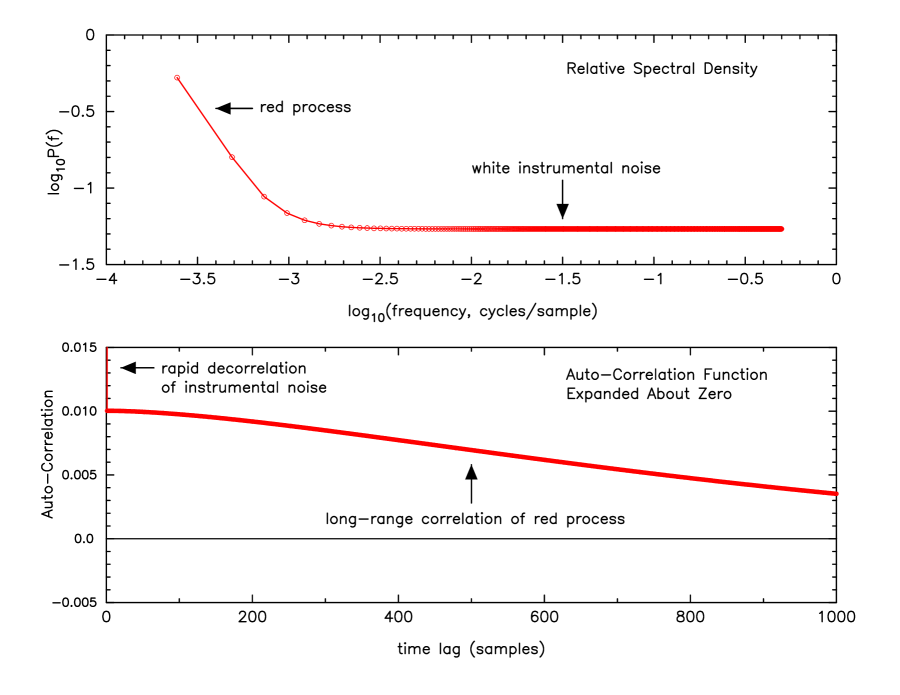
Figure 1: Schematic illustration of the method. The upper panel shows the power spectrum of (assumed-white) instrumental noise plus a low-frequency excess (”red”) signal power. The lower panel shows the auto-correlation function of the spectrum in the upper panel, expanded around zero correlation. The white component decorrelates rapidly from unity, while the red process gives rise to long-range correlations. The detection of these correlations competes with estimation error statistics of the correlation function, with an SNR increasing like $T^{1/2}$, as described in the text.

From the statistical properties of both the GW stochastic background and the noise, and by taking into account the central-limit theorem (for $\tau_{\rm gw}<<T$, $S(\tau)$ is equal to the sum of many uncorrelated products) it follows that $S(\tau)$ is also a Gaussian random process Papoulis2002 . In order to fully characterize it we can estimate its mean and variance, which must be functions of only the spectra of the two random processes $h(t)$ and $n(t)$.

By taking the ensemble average of $S$ and $S^{2}$ over many noise and GW signal realizations and for $T>>\tau_{\rm gw}$, after some long but straightforward calculations we get the following expressions for the mean and variance of $S(\tau)$ (see Appendix A for details)

$$\mu_{S}\equiv\langle S\rangle=\frac{T}{2}\ \int^{\infty}_{-\infty}P_{h}(|f|)e^{2\pi if\tau}\ df\ ,$$ (5)

$$\sigma^{2}_{S}\equiv\langle S^{2}\rangle-\langle S\rangle^{2}=\frac{T}{2}\ \int^{\infty}_{-\infty}\cos^{2}(2\pi f\tau)\ [P_{h}(|f|)+P_{n}(|f|)]^{2}\ df\ .$$ (6)

Eqs.(5, 6) can then be used for deriving the following expression for the Signal-to-Noise Ratio ($SNR_{auto}$)

$$SNR_{auto}\equiv\frac{\mu_{S}}{\sigma_{S}}=\sqrt{\frac{T}{2}}\ \frac{\int^{\infty}_{-\infty}P_{h}(|f|)e^{2\pi if\tau}\ df}{\left[\int^{\infty}_{-\infty}\cos^{2}(2\pi f\tau)\ [P_{h}(|f|)+P_{n}(|f|)]^{2}\ df\right]^{1/2}}\ .$$ (7)

In order to get a quantitative understanding of the above expression for the SNR of the auto-correlation at lag $\tau$, we may compare it against the SNR associated with the cross-correlation (computed also at time-lag $\tau$) of the data from two co-aligned and co-located detectors whose noises are assumed to be uncorrelated (see AllenRomano1999 for details). It is straightforward to obtain the following expression for the cross-correlation signal-to-noise ratio $SNR_{2d}$

$$SNR_{2d}=\sqrt{\frac{T}{2}}\ \frac{\int^{\infty}_{-\infty}P_{h}(|f|)e^{2\pi if\tau}\ df}{\left[\int^{\infty}_{-\infty}\left[P_{h}^{2}(|f|)\cos^{2}(2\pi f\tau)+\frac{1}{2}P_{h}(|f|)\ (P_{1n}(|f|)+P_{2n}(|f|))+\frac{1}{2}P_{1n}(|f|)P_{2n}(|f|)\right]\right]^{1/2}}\ ,$$ (8)

where we have denoted with $P_{in}(|f|)$ the one-sided power spectral density of the noise in detector $i=1,2$. In order to compare the two expressions given in Eqs. (7, 8), let us assume the two noise power spectral densities $P_{in}$ to be equal to each other and to a white spectrum having spectral level equal to $A$ per unit bandwidth. By taking the ratio between $SNR_{2d}$ and $SNR_{auto}$ we get

$$\frac{SNR_{2d}}{SNR_{auto}}=\frac{\left[\int^{\infty}_{-\infty}\cos^{2}(2\pi f\tau)\ [P_{h}(|f|)+A]^{2}\ df\right]^{1/2}}{\left[\int^{\infty}_{-\infty}\left[P_{h}^{2}(|f|)\cos^{2}(2\pi f\tau)+P_{h}(|f|)\ A+\frac{1}{2}A^{2}\right]\right]^{1/2}}\ .$$ (9)

Since current estimates for the likely amplitudes of cosmological gravitational wave backgrounds indicate them to be significantly smaller than the instrumental noise levels of current and future detectors, if we take $P_{h}<<A$ in Eq. (9) in this limit we find $SNR_{2d}/SNR_{auto}\rightarrow 1$.

II.1 The optimal filter

Although the physical reasons underlying the selection of the time interval within which the time-lag $\tau$ should be selected are quite clear, they do not allow us to uniquely identify a value for it. In particular, since the number of possible time lags we could use for estimating the auto-correlation function can be in general rather large, it is natural to look for the optimal way of combining all possible auto-correlation functions. In analogy with the cross-correlation technique AllenRomano1999 in which an optimal filter $Q(t,t^{\prime})$ maximizing the SNR could be identified, here we show that also for the auto-correlation technique there exists such a filter. Since the stochastic background and the instrumental noise have been assumed to be stationary, we introduce a time-invariant filter function and write the following linear combination of all possible sample auto-correlation functions lags

$${\mathcal{S}}\equiv\int^{T/2}_{-T/2}\ \int^{+\infty}_{-\infty}\ R(t)R(t+\tau)Q(\tau)\ dt\ d\tau\ ,$$ (10)

where the auto-correlation is computed over the time interval $T$, and the filter function $Q(\tau)$ at the time-lag $\tau$ is non-zero in the interval $\tau_{n}<|\tau|<\tau_{gw}$ and zero everywhere else (a property that we have already taken into account in Eq. (10) by extending the $\tau$-integration over the entire real axis).

From the statistical properties of both the GW stochastic background and the noise, and by virtue of the central-limit theorem, it follows that $\mathcal{S}$ is also a Gaussian random process Papoulis2002 that can be fully characterized by estimating its mean $\mu_{\mathcal{S}}$ and variance, $\sigma^{2}_{\mathcal{S}}$. Although their derivations are quite long, they are straightforward and result into the two following expressions

$$\mu_{\mathcal{S}}=\frac{T}{2}\int^{+\infty}_{-\infty}P_{h}(|f|)\ {\widetilde{Q}}(f)\ df\ ,$$ (11)

$$\sigma^{2}_{\mathcal{S}}=\frac{T}{2}\int^{+\infty}_{-\infty}[P_{h}(|f|)+P_{n}(|f|)]^{2}\ |{\widetilde{Q}}(f)|^{2}\ df\ .$$ (12)

By simple inspection of Eq. (12), and following AllenRomano1999 , it is convenient to define the following operation of inner product between two arbitrary complex functions, say $A$, and $B$

$$(A,B)\equiv\int^{+\infty}_{-\infty}A(f)B^{*}(f)[P_{h}(|f|)+P_{n}(|f|)]^{2}\ df\ .$$ (13)

With this newly defined inner product, $\mu_{\mathcal{S}}$ and $\sigma_{\mathcal{S}}$ can be rewritten in the following form

$$\mu_{\mathcal{S}}=\frac{T}{2}({\widetilde{Q}},\frac{P_{h}}{[P_{h}+P_{n}]^{2}})\ \ \ \ ;\ \ \ \ \sigma^{2}_{\mathcal{S}}=\frac{T}{2}(Q,Q)\ ,$$ (14)

while the squared signal-to-noise ratio of $\mathcal{S}$, $SNR^{2}$ is equal to

$$SNR^{2}\equiv\frac{\mu_{\mathcal{S}}^{2}}{\sigma^{2}_{\mathcal{S}}}=\frac{T}{2}\ \frac{({\widetilde{Q}},\frac{P_{h}}{[P_{h}+P_{n}]^{2}})^{2}}{(Q,Q)}\ .$$ (15)

From a simple geometrical interpretation of the inner product defined through Eq. (13), from Eq. (15) it is easy to see that the maximum of the SNR of $\mathcal{S}$ is achieved by choosing the filter function ${\widetilde{Q}}$ to be equal to

$${\widetilde{Q}}(f)=\lambda\ \frac{P_{h}(|f|)}{[P_{h}(|f|)+P_{n}(|f|)]^{2}}\ ,$$ (16)

where $\lambda$ can be any arbitrary real number. The above expression for the filter $Q$ implies the following maximum SNR achievable by the auto-correlation technique

$$SNR^{2}_{max}=\frac{T}{2}\int^{+\infty}_{-\infty}\frac{P_{h}^{2}(|f|)}{[P_{h}(|f|)+P_{n}(|f|)]^{2}}\ df\ .$$ (17)

III Discussions and conclusions

The main result of our work has been to show that the auto-correlation function of the data measured by a single detector of gravitational radiation can be used for searching for a stochastic gravitational wave background. This is possible when there is a difference between the spectral properties of the GW background and of the instrumental noise. By estimating the auto-correlation function of the data at a time-lag at which the auto-correlation of the noise has decayed to a value smaller than that of the auto-correlation function of the GW background, one can enhance the resulting power signal-to-noise ratio by the square-root of the integration time.

We have assessed the effectiveness of our technique by comparing the expression of its SNR against that achievable by cross-correlating the data from two co-located and co-aligned detectors whose noises are assumed to be uncorrelated. We found the two expressions to coincide in the expected limit of the noise power spectrum larger than that of the GW background. In order to further enhance the SNR associated with the auto-correlation technique we have derived the expression of an optimal filter function that reflects any prior knowledge we might have about the spectrum of GW background.

The auto-correlation technique can be used when searching for a stochastic background of gravitational radiation with (i) networks of ground-based interferometer as it will further enhance the likelihood of detection achievable with the cross-correlation method, (ii) with a single space-based interferometer, and (iii) with pulsar timing data.

Appendix A Derivation of the mean and variance of $S(\tau)$

In what follows we derive the expressions of the mean and variance of the auto-correlation function $S(\tau)$ (Eqs. (5, 6) given in Section (II)). We will assume the instrumental noise to be characterized by a random process $n(t)$ that is Gaussian-distributed with zero-mean, and has one-sided power-spectral density $P_{n}(|f|)$. We will also take the GW stochastic background to be a Gaussian random process of zero-mean, unpolarized, and stationary. As a consequence of these assumptions such a background is uniquely characterized by a one-sided power spectral density, $P_{h}(|f|)$ as given by Eq. (2).

From the definitions of the data, $R(t)$, and of the auto-correlation function, $S(\tau)$, calculated at a time-lag $\tau$ such that $\tau_{n}<\tau<\tau_{\rm gw}$, we have

$$S(\tau)\equiv\int^{T/2}_{-T/2}[h(t)+n(t)]\ [h(t+\tau)+n(t+\tau)]\ dt\ ,$$ (18)

where $T$ is the time interval in seconds over which the auto-correlation function is computed and it is assumed to be longer than $\tau_{\rm gw}$. After taking the ensemble average of both sides of Eq. (18), we get

$$\langle S(\tau)\rangle=\int^{T/2}_{-T/2}\left[\langle h(t)h(t+\tau)\rangle+\langle h(t)n(t+\tau)\rangle+\langle n(t)h(t+\tau)\rangle+\langle n(t)n(t+\tau)\rangle\right]\ dt\ .$$ (19)

Note that the second and third terms on the right-hand-side of Eq. (19) are equal to zero because the random process associated with the stochastic GW background and that associated with the instrumental noise are uncorrelated. The fourth term instead can also be regarded to be zero because is the auto-correlation function of the noise estimated at an off-set time longer than its coherence time. From these considerations we find the following expression for the mean of $S$

$$\mu_{S}\equiv\langle S(\tau)\rangle=\int^{T/2}_{-T/2}\left[\langle h(t)h(t+\tau)\rangle\right]\ dt\ =\frac{T}{2}\int_{-\infty}^{+\infty}P_{h}(|f|)e^{2\pi if\tau}\ df\ .$$ (20)

In order to derive the expression for the variance of $S$ (Eq. (6)) we need to calculate $\langle S^{2}\rangle$. Since $S^{2}(\tau)$ can be written as

$$S^{2}(\tau) = \int^{T/2}_{-T/2}\int^{T/2}_{-T/2}\left[h(t)h(t+\tau)+h(t)n(t+\tau)+n(t)h(t+\tau)+n(t)n(t+\tau)\right]$$ (21)

$$\times \left[h(t^{\prime})h(t^{\prime}+\tau)+h(t^{\prime})n(t^{\prime}+\tau)+n(t^{\prime})h(t^{\prime}+\tau)+n(t^{\prime})n(t^{\prime}+\tau)\right]\ dt\ dt^{\prime}\ ,$$

by taking the ensemble average of both sides of Eq. (21) only nine of the sixteen terms present are different from zero. This follows from the Gaussian nature of both random processes and because terms such as $\langle x(t)y(t^{\prime})z(t+\tau)w(t^{\prime}+\tau)\rangle$ (where $x,y,z,w$ can be either $h$ or $n$) can be expressed in the following form Papoulis2002

$$\langle x(t)y(t^{\prime})z(t+\tau)w(t^{\prime}+\tau)\rangle = \langle x(t)y(t^{\prime})\rangle\langle z(t+\tau)w(t^{\prime}+\tau)\rangle+\langle x(t)z(t+\tau)\rangle\langle y(t^{\prime})w(t^{\prime}+\tau)\rangle$$ (22)

$$+ \langle x(t)w(t^{\prime}+\tau)\rangle\langle y(t^{\prime})z(t+\tau)\rangle$$

From the above considerations we get the following expression for $\langle S^{2}(\tau)\rangle$

$$\langle S^{2}(\tau)\rangle = \int^{T/2}_{-T/2}\int^{T/2}_{-T/2}\left[\langle h(t)h(t+\tau)\rangle\langle h(t^{\prime})h(t^{\prime}+\tau)\rangle+\langle h(t)h(t^{\prime})\rangle\langle h(t+\tau)h(t^{\prime}+\tau)\rangle\right.$$ (23)

$$+ \left.\langle h(t)h(t^{\prime}+\tau)\rangle\langle h(t^{\prime})h(t+\tau)\rangle+\langle h(t)h(t^{\prime})\rangle\langle n(t+\tau)n(t^{\prime}+\tau)\rangle\right.$$

$$+ \left.\langle h(t)h(t^{\prime}+\tau)\rangle\langle n(t+\tau)n(t^{\prime})\rangle+\langle h(t^{\prime})h(t+\tau)\rangle\langle n(t)n(t^{\prime}+\tau)\rangle\right.$$

$$+ \left.\langle h(t+\tau)h(t^{\prime}+\tau)\rangle\langle n(t)n(t^{\prime})\rangle+\langle n(t)n(t^{\prime})\rangle\langle n(t+\tau)n(t^{\prime}+\tau)\rangle\right.$$

$$+ \left.\langle n(t)n(t^{\prime}+\tau)\rangle\langle n(t^{\prime})n(t+\tau)\rangle\right]\ dt\ dt^{\prime}\ ,$$

which can further be rewritten in the following form

$$\langle S^{2}(\tau)\rangle = \frac{T^{2}}{4}\int^{+\infty}_{-\infty}\int^{+\infty}_{-\infty}P_{h}(|f|)P_{h}(|f^{\prime}|)\ e^{2\pi i(f-f^{\prime})\tau}\ df\ df^{\prime}+\frac{T}{4}\int^{+\infty}_{-\infty}P^{2}_{h}(|f|)\ df$$ (24)

$$+ \frac{T}{4}\int^{+\infty}_{-\infty}P^{2}_{h}(|f|)e^{4\pi if\tau}\ df+\frac{T}{4}\int^{+\infty}_{-\infty}P_{h}(|f|)P_{n}(|f|)\ df$$

$$+ \frac{T}{4}\int^{+\infty}_{-\infty}P_{h}(|f|)P_{n}(|f|)e^{4\pi if\tau}\ df+\frac{T}{4}\int^{+\infty}_{-\infty}P_{h}(|f|)P_{n}(|f|)e^{-4\pi if\tau}\ df$$

$$+ \frac{T}{4}\int^{+\infty}_{-\infty}P_{h}(|f|)P_{n}(|f|)\ df+\frac{T}{4}\int^{+\infty}_{-\infty}P^{2}_{n}(|f|)\ df$$

$$+ \frac{T}{4}\int^{+\infty}_{-\infty}P^{2}_{n}(|f|)e^{4\pi if\tau}\ df\ .$$

If we now square both sides of Eq. (20) and subtract it from Eq. (24) to obtain the expression for the variance $\sigma^{2}_{S}$, after some rearrangement of the remaining terms we get the following result

$$\sigma^{2}_{S}=\frac{T}{2}\int^{+\infty}_{-\infty}\cos^{2}(2\pi f\tau)[P_{h}(|f|)+P_{n}(|f|)]^{2}\ df\ .$$ (25)

References

- (1) K.S. Thorne. In: Three Hundred Years of Gravitation, 330-458, Eds. S.W. Hawking, and W. Israel (Cambridge University Press: New York), (1987).
- (2) http://www.ligo.caltech.edu/ .
- (3) http://www.virgo.infn.it/ .
- (4) http://www.geo600.uni-hannover.de/ .
- (5) http://tamago.mtk.nao.ac.jp/ .
- (6) J.W. Armstrong, Living Rev. Relativity, 9, (2006).
- (7) P. Bender, K. Danzmann, & the LISA Study Team, Laser Interferometer Space Antenna for the Detection of Gravitational Waves, Pre-Phase A Report, MPQ233 (Max-Planck- Institüt für Quantenoptik, Garching), July 1998.
- (8) S. Detweiler, Ap. J., 234, 1100-1104 (1979).
- (9) F.A. Jenet, J.W. Armstrong and M. Tinto, Phys. Rev. D, 83, 081301, (2011).
- (10) B. Allen, and J.D. Romano, Phys. Rev. D, 59, 102001 (1999).
- (11) M. Tinto, and S.V. Dhurandhar, Living Rev. Relativity, 8 (2005), 4.
- (12) T.A. Prince, M. Tinto, S.L. Larson, and J.W. Armstrong, Phys. Rev. D, 66, 122002, (2002).
- (13) M. Tinto, J.W. Armstrong, and F.B. Estabrook, Phys. Rev. D, 63 021101, (2000).
- (14) E.L. Robinson, J.D. Romano, and A. Vecchio, Class. Quantum Grav., 25, 184019, (2008).
- (15) A. Papoulis, Probability, random variables, and stochastic processes, third edition, McGraw-Hill, Inc, New York (1991)
- (16) S. Mitra, S. Dhurandhar, T. Souradeep, A. Lazzarini, V. Mandic, S. Bose, and S. Ballmer, Phys. Rev. D, 77, 042002, (2008).
- (17) G.M. Jenkins and D.G. Watts, Spectral Analysis and its Applications, Holden-Day, Inc., New York (1968)