The role of the supermassive black hole spin in the estimation of the EMRI event rate

Abstract

One of the main channels of interactions in galactic nuclei between stars and the central massive black hole (MBH) is the gradual inspiral of compact remnants into the MBH due to the emission of gravitational radiation. This process is known as an “Extreme Mass Ratio Inspiral” (EMRI). Previous works about the estimation of how many events space observatories such as LISA will be able to observe during its operational time differ in orders of magnitude, due to the complexity of the problem. Nevertheless, a common result to all investigations is that the possibility that a compact object merges with the MBH after only one intense burst of GWs is much more likely than a slow adiabatic inspiral, an EMRI. The later is referred to as a “plunge” because the compact object dives into the MBH, crosses the horizon and is lost as a probe of strong gravity for eLISA. The event rates for plunges are orders of magnitude larger than slow inspirals. On the other hand, nature MBH’s are most likely Kerr and the magnitude of the spin has been sized up to be high. We calculate the number of periapsis passages that a compact object set on to an extremely radial orbit goes through before being actually swallowed by the Kerr MBH and we then translate it into an event rate for a LISA-like observatory, such as the proposed ESA mission eLISA/NGO. We prove that a “plunging” compact object is conceptually indistinguishable from an adiabatic, slow inspiral; plunges spend on average up to hundred of thousands of cycles in the bandwidth of the detector for a two years mission. This has an important impact on the event rate, enhancing in some cases significantly, depending on the spin of the MBH and the inclination: If the orbit of the EMRI is prograde, the effective size of the MBH becomes smaller the larger the spin is, whilst if retrograde, it becomes bigger. However, this situation is not symmetric, resulting in an effective enhancement of the rates. The effect of vectorial resonant relaxation on the sense of the orbit does not affect the enhancement. Moreover, it has been recently proved that the production of low-eccentricity EMRIs is severely blocked by the presence of a blockade in the rate at which orbital angular momenta change takes place. This is the result of relativistic precession on to the stellar potential torques and hence affects EMRIs originating via resonant relaxation at distances of about $\sim 10^{-2}$ pc from the MBH. Since high-eccentricity EMRIs are a result of two-body relaxation, they are not affected by this phenomenon. Therefore we predict that eLISA EMRI event rates will be dominated by high-eccentricity binaries, as we present here.

1 Motivation

We know, mostly through high-resolution observations of the kinematics of stars and gas, that most, if not all, nearby bright galaxies harbour a dark, massive, compact object at their centres. (Ferrarese & Ford 2005; Kormendy 2004). The most spectacular case is our own galaxy, the Milky Way. By tracking and interpreting the stellar dynamics at the centre of our galaxy, we have the most well-established evidence for the existence of a massive black hole (MBH) (Eisenhauer et al. 2005; Ghez et al. 2005, 2008; Gillessen et al. 2009). Observations of other galaxies indicate that the masses of MBH can reach a few billion solar masses ($M_{\odot}$). The existence of such a MBH population in the present-day universe is strongly supported by Sołtan’s argument that the average mass density of these MBHs agrees with expectations from integrated luminosity of quasars (Sołtan 1982; Yu & Tremaine 2002). Many correlations linking the MBH’s mass and overall properties of its host spheroid (bulge or elliptical galaxy) have been discovered. The tightest are with the spheroid mass (Häring & Rix 2004), its velocity dispersion ($M-\sigma$ relation, Tremaine et al. 2002) and degree of concentration (Erwin et al. 2004). Consequently, understanding the origin and evolution of these MBHs necessitates their study in the context of their surrounding stellar systems.

The ideal probe of these regions is the gravitational radiation (GWs) that is emitted by some compact stars very close to the black holes, and which will be surveyed by eLISA/NGO (evolved Laser Interferometer Space Antenna / New Gravitational Wave Observatory Amaro-Seoane et al. 2012a, b). This mission will scrutinise the range of masses fundamental to the understanding of the origin and growth of supermassive black holes; i.e. MBHs with masses below $10^{7}\,M_{\odot}$.

2 EMRIs and direct plunges

For a binary of a MBH and a stellar black hole to be in a LISA-like band, it has to have a frequency of between roughly $1$ and $10^{-5}$ Hz. The emission of GWs is more efficient as they approach the LSO, so that the observatory will detect the sources when they are close to the LSO line. The total mass required to observe systems with frequencies between $0.1$ Hz and $10^{-4}$ Hz is of $10^{4}-10^{7}\,M_{\odot}$. For masses larger than $10^{7}\,M_{\odot}$ the frequencies close to the LSO will be too low, so that their detection will be very difficult. On the other hand, for a total mass of less than $10^{3}\,M_{\odot}$ we could in principal detect them at an early stage, but then the amplitude of the GW would be rather low.

To interact closely with the central MBH, stars have to find themselves on “loss-cone” orbits, which are orbits elongated enough to have a very close-in periapsis (Frank & Rees 1976; Lightman & Shapiro 1977; Amaro-Seoane & Spurzem 2001). The rate of tidal disruptions can be established semi-/analytically if the phase space distribution of stars around the MBH is known (Magorrian & Tremaine 1999; Syer & Ulmer 1999; Wang & Merritt 2004, for estimates in models of observed nearby nuclei). To account for the complex influence of mass segregation, collisions and the evolution of the nucleus over billions of years, detailed numerical simulations are required, however (David et al. 1987a, b; Murphy et al. 1991; Freitag & Benz 2002; Baumgardt et al. 2004; Amaro-Seoane 2004; Freitag et al. 2006; Khalisi et al. 2007; Preto & Amaro-Seoane 2010; Amaro-Seoane & Preto 2011).

As the star spirals down towards the MBH, it has many opportunities to be deflected back by two-body encounters onto a “safer orbit” (Alexander & Hopman 2003; Amaro-Seoane et al. 2007), hence even the definition of a loss cone is not straightforward. Once again, the problem is compounded by the effects of mass segregation and resonant relaxation, to mention two main complications. As a result, considerable uncertainties are attached to the (semi-)analytical predictions of capture rates and orbital parameters of EMRIs.

Naively one could assume that the inspiral time is dominated by GW emission and that if this is shorter than a Hubble time, the compact object will become an EMRI. This is wrong, because one has to take into account the relaxation of the stellar system. Whilst it certainly can increase the eccentricity of the compact object, it can also perturb the orbit and circularise it, so that the required time to inspiral in, $t_{\rm GW}$, becomes larger than a Hubble time. The condition for the small compact object to be an EMRI is that it is on an orbit for which $t_{\rm GW}\ll(1-e)\,t_{\rm r}$ (Amaro-Seoane et al. 2007), with $t_{\rm r}$ the local relaxation time. When the binary has a semi-major axis for which the condition is not fulfilled, the small compact object will have to be already on a so-called “plunging orbit”, with $e\geq e_{\rm plunge}\equiv 1-4\,R_{\rm Schw}/a$, where $R_{\rm Schw}$ is the Schwarzschild radius of the MBH, i.e. $R_{\rm Schw}=2GM_{\bullet}/c^{2}$, with $M_{\bullet}$ being the MBH mass. It has been claimed a number of times by different authors that this would result in a too short burst of gravitational radiation which could only be detected if it was originated in our own Galactic Center (Hopman et al. 2007), because one needs a coherent integration of some few thousands repeated passages through the periapsis in the eLISA bandwidth.

Therefore, such “plunging” objects would then be lost for the GW signal, since they would be plunging “directly” through the horizon of the MBH and only a final burst of GWs would be emitted, and such burst would be (i) very difficult to recover, since the very short signal would be buried in a sea of instrumental and confusion noise and (ii) the information contained in the signal would be practically nil. There has been some work on the detectability of such bursts (Rubbo et al. 2006; Hopman et al. 2007; Yunes et al. 2008; Berry & Gair 2012), but they would only be detectable in our galaxy or in the close neighborhood, but the event rates are rather low, even in the most optimistic scenarios.

The typical size of the central MBH can be associated with the gravitational radius (radial horizon location) of the MBH, which in the case of the Milky Way MBH corresponds to approximately $R_{\rm Schw}\sim 1.3\times 10^{7}$ km $\approx 4.1\times 10^{-7}$ pc (neglecting spin contributions). This number gives a good indication of how small are these MBHs in size, which means they have a small cross section and hence, the chances a star has to “plunge” through the horizon of the MBH directly are very small.

To quantify the probability for star absorption by a MBH it is crucial to take into account the location of the Last Stable Orbit (LSO) of a test massive body in terms of the MBH parameters. According to General Relativity, these are the mass $M_{\bullet}$ and its intrinsic angular momentum or spin $S_{\bullet}=a_{\bullet}\,M_{\bullet}c$, where $a_{\bullet}$ is the spin parameter with length dimension and subject to the constraints $0\leq a_{\bullet}c^{2}/(GM_{\bullet})\leq 1$. The LSO location is given by a surface in the orbital configuration space that can be described in terms of the parameters $(p,e,\iota)$, where $p$ is the dimensionless semilatus rectum, $e$ is the eccentricity, and $\iota$ is the orbital inclination (with respect to the MBH spin axis) of the orbit. Equivalently one can also use the semimajor axis $a$, or the periapsis location $r_{\rm peri}$, instead of $p$. The periapsis and apoapsis radii are given then by:

$$r_{\rm peri} =\frac{GM_{\bullet}\,p}{c^{2}(1+e)}\,,$$

$$r_{\rm apo} =\frac{GM_{\bullet}\,p}{c^{2}(1-e)}\,.$$ (1)

It is well-known (see e.g. Bardeen 1970) that the LSO, for the case of circular orbits, lies at $3\,R_{\rm Schw}$ for non-spinning MBHs, while it is shifted out to $9GM_{\bullet}/c^{2}$ for retrograde orbits and down to $GM_{\bullet}/c^{2}$ for prograde orbits, and these values correspond to the case of “extremal” MBHs, characterized by maximal spins, i.e. $a_{\bullet}c^{2}/(GM_{\bullet})=1\,$. Despite this fact, traditional EMRI event rate estimations are based on considerations that neglect the spin of the MBH. Taking into account the spin one would expect (considering the asymmetry between prograde and retrograde orbits) an increase of the number of EMRIs since some of the traditionally neglected “direct plunges” can actually be disguised EMRIs.

3 Orbital geodesic motion around a Kerr MBH

In order to show the importance of the effect of the spin in the estimation of the number of EMRIs that will produce a significant amount of GW cycles in the band of eLISA, we present here two types of calculations. The first one is to adapt known results about the stability of orbits of massive objects around a MBH to our discussion. The second is an estimation of the number of cycles for for orbits which would be plunging orbits for a Schwarzschild MBH, or orbits with no sufficient cycles when the MBH was assumed to be non-spinning for the case with spin. We show that a significant fraction of them are actually EMRIs with sufficient cycles to be detected by a space-based observatory like eLISA. Parts of these calculations, mainly due to the high eccentricities involved, require numerical computations.

At this point it is useful to review some basic characteristics of the orbital geodesic motion of massive bodies around a Kerr MBH. First of all, the geometry of a Kerr MBH is axisymmetric (with respect to the spin axis) instead of spherically-symmetric as in the case of Schwarzschild MBHs, and this means that the inclination of the orbit with respect to the spin axis, $\iota$, plays an important role in the dynamics. Actually, orbits outside the equatorial plane are not planar, like in Keplerian motion or orbits around a Schwarzschild MBH, but instead they would precess around a plane with a certain inclination $\iota$ with a frequency that we call $f_{\theta}$, where $\theta$ refers to the polar Boyer-Lindquist coordinate of the MBH (Boyer & Lindquist 1967; Misner et al. 1973). In addition, relativistic effects cause precession of the periapsis, and this already happens for Schwarzschild MBHs, so that we have to consider two more frequencies, $f_{r}$ and $f_{\varphi}$. The first one, $f_{r}$, is associated with the radial motion and the time to go from periapsis, $r_{\rm peri}$, to apoapsis, $r_{\rm apo}$, and back. The second one, $f_{\varphi}$, is associated with the azimuthal motion around the spin axis and the time to complete a full turn ($2\,\pi$) around this axis, or in other words, the time for the azimuthal angle $\varphi$ to increase $2\pi$ radians.

In summary, generic bound motion around a Kerr MBH exhibits three fundamental frequencies, $(f_{r},\,f_{\theta},\,f_{\varphi})$ and this implies that the GW emission of an EMRI will be quite rich in structure (not only these GWs will contain features with these frequencies but also with a number of harmonics of them), encoding the detailed geometry of the central Kerr MBH. The GW emission will back react on to the system and this translates in particular in a change of the orbital parameters $(p,\,e,\,\iota)$ of the orbit. These changes can be estimated by considering the energy and angular momentum carried away from the extreme-mass-ratio binary by the GWs emitted. More specifically, the GW emission changes the constants of motion of the geodesic motion, namely the energy per unit mass (normalized with respect to the star mass, $m$), $E$, the angular momentum along the spin axis per unit mass, $L_{z}$, and the so-called Carter constant per unit mass square, $C$, which is associated with an extra symmetry of the Kerr geometry, similar to what happens in certain axisymmetric Newtonian potentials (Binney & Tremaine 1987). Actually, the set of constants $(E,L_{z},C)$ parametrizes the geodesic orbit in the same way as the set of orbital parameters $(p,e,\iota)$ does. Therefore, there is a mapping between these two sets (see Schmidt 2002) which is going to be crucial in the calculations that we present here. The explicit form of this mapping is quite complex and we do not include it here, we just mention that we used the implementation described in Sopuerta & Yunes (2011).

In the case of a non-spinning Schwarzschild MBH, where $\iota$ and $C$ do not play any role, the mapping is much more simple and is given by:

$$\frac{E^{2}}{c^{2}}= \frac{(p-2-2e)(p-2+2e)}{p\,(p-3-e^{2})}\,,$$ (2)

$$L^{2}_{z}= \frac{G^{2}M^{2}_{\bullet}\,p^{2}}{c^{2}(p-3-e^{2})}\,.$$ (3)

Using the symmetries of the geometry of a Kerr MBH we can separate the equations for geodesic orbital motion so that the trajectory of a massive body, described in terms of Boyer-Lindquist coordinates $\{t,r,\theta,\varphi\}$, can be written as follows

$$\rho^{2}\,\frac{d{t}}{d\tau} =\frac{1}{\Delta}\left(\Sigma^{2}\frac{E}{c}-2a_{\bullet}r_{\bullet}\frac{{L}_{z}}{c}r\right)$$ (4)

$$\rho^{4}\,\left(\frac{d{r}}{d\tau}\right)^{2} =\left[\left(r^{2}+a^{2}_{\bullet}\right)\frac{E}{c}-a_{\bullet}\frac{L_{z}}{c}\right]^{2}-$$

$$\left(\frac{Q}{c^{2}}+r^{2}\right)\Delta\equiv R(r)$$ (5)

$$\rho^{4}\,\left(\frac{d{\theta}}{d\tau}\right)^{2} =\frac{C}{c^{2}}-\frac{{L}^{2}_{z}}{c^{2}}\cot^{2}{\theta}-a^{2}_{\bullet}\left(1-\frac{{E}^{2}}{c^{2}}\right)\cos^{2}{\theta}$$ (6)

$$\rho^{2}\,\frac{d\varphi}{d{\tau}} =\frac{1}{\Delta}\left[2a_{\bullet}r_{\bullet}\frac{E}{c}r+\frac{{L}_{z}}{c}\frac{\Delta-a^{2}_{\bullet}{\sin^{2}{\theta}}}{\sin^{2}\theta}\right].$$ (7)

In the last set of equations we have introduced the following definitions:

$$r_{\bullet} \equiv\frac{GM_{\bullet}}{c^{2}},$$

$$Q \equiv C+\left(L_{z}-a_{\bullet}E\right)^{2},$$

$$\rho^{2} \equiv r^{2}+a^{2}_{\bullet}\cos^{2}{\theta}$$

$$\Delta \equiv r^{2}-2r_{\bullet}r+a^{2}_{\bullet}=r^{2}f+a^{2}_{\bullet},{\rm~{}with~{}}f\equiv 1-\frac{2\,r_{\bullet}}{r}.$$ (8)

For convenience, we also define the quantity $\Sigma^{2}\equiv(r^{2}+a^{2}_{\bullet})^{2}-a^{2}_{\bullet}\Delta\,\sin^{2}\theta\,$. The first equation tells us how the coordinate time $t$ changes with respect to the proper time $\tau$ and the other three describe the trajectory in space. One can combine the four equations to obtain the spatial trajectory in terms of coordinate time $t$, the time of observers at infinity, i.e. $(r(t),\theta(t),\varphi(t))$.

4 Kerr and Schwarzschild separatrices

In figures 1 and 2 we show plots of the location of the LSO in the plane $a$ (pc) - $(1-e)$, including the Schwarzschild separatrix between stable and unstable orbits, $p-6-2e=0$, for both prograde and retrograde orbits and for different values of the inclination $\iota$. Each plot corresponds to a different value of the spin, showing how increasing the spin makes a difference in shifting the location of the separatrix between stable and unstable orbits, pushing prograde orbits near $GM_{\bullet}/c^{2}$ while retrograde orbits are pushed out towards $9GM_{\bullet}/c^{2}$. The procedure we have used to build these plots is a standard one. Briefly, given a value of the dimensionless spin parameter $s\equiv a_{\bullet}c^{2}/(GM_{\bullet})$ and a value of the eccentricity $e$ and inclination angle $\iota$ we apply the following algorithm:

1. We start from an initial value of the semilatus rectum $p$ which, together with the value of the eccentricity fixes the apoapsis and periapsis radii through the equations in (1). On the other hand, the inclination of the orbital plane can also be described in terms of the polar angle $\theta$, so that $\theta_{\rm inc}$ represents the inclination angle and is closely related to $\iota$ (see e.g., Drasco & Hughes 2004). The advantage of using $\theta_{\rm inc}$ is that it is related in a simple way to the extrema of $\theta$, $\theta_{\rm min}$ satisfying –see equation (6)

   $$\left(\frac{d\theta}{d\tau}\right)_{\theta=\theta_{\rm min}}=0\,,$$ (9)

   by $\theta_{\rm inc}={\rm sign}(L_{z})\left(\frac{\pi}{2}-\theta_{\rm min}\right)$, with

   $${\rm sign}(L_{z})=\begin{cases}+1&\text{for prograde orbits\,,}\\ -1&\text{for retrograde orbits\,.}\end{cases}$$ (10)

   Then, from the condition of extrema of $\theta_{\rm min}$ and its relation to $\theta_{\rm inc}$, we can find the value of the Carter constant $C$ in terms of the energy $E$ and angular momentum along the spin axis $L_{z}$.

2. From the conditions of extrema of periapsis and apoapsis,

   $$\left(\frac{dr}{d\tau}\right)_{r=r_{\rm peri}}=\left(\frac{dr}{d\tau}\right)_{r=r_{\rm apo}}=0,$$ (11)

   [see equation (5)], and using the expression of $C$ in terms of $(E,L_{z})$ from the previous point, we find the values of $(E,L_{z})$ (and hence of $C$ too).

3. The radial motion for geodesic orbits around Kerr has four extrema, the periapsis and apoapsis locations and two more radii, $r_{3}$ and $r_{4}$, such that

   $$r_{\rm apo}\geq r_{\rm peri}\geq r_{\rm 3}>r_{4}.$$ (12)

   Actually, $r_{4}$ always lies inside the horizon radius,

   $$r_{\rm H}=\left(\frac{GM_{\bullet}}{c^{2}}\right)\left(1+\sqrt{1-s^{2}}\right),$$ (13)

   i.e. $r_{4}<r_{\rm H}$. For any stable orbit, it is obvious that the radial motion happens inside the interval $[r_{\rm peri},\,r_{\rm apo}]$. However, for orbital configurations with $r_{\rm peri}=r_{3}$, the potential of the MBH changes its shape and the orbits become unstable, marking the location of the LSO. In this case, we have that

   $$\left(\frac{dR(r)}{dr}\right)_{r=r_{3}}=0,$$ (14)

   where $R(r)$ denotes the right-hand side of the evolution equation for the radial position $r$ (see equation 5).

The calculations in this algorithm are done numerically, so we check whether this condition is satisfied to some tolerance level. In the case it is not satisfied, we use this information to prescribe the next value of $p$ and come back to the first point in the algorithm. The process is repeated until we identify the LSO with the desired accuracy.

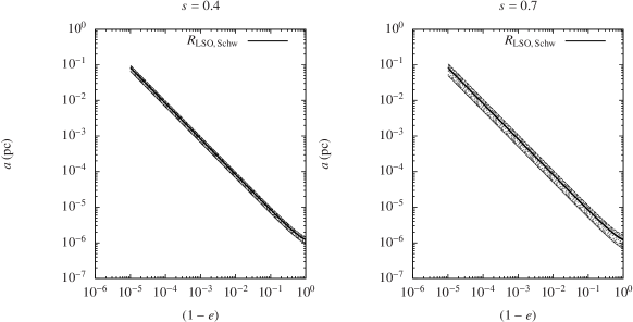
Figure 1: LSO for a MBH of mass $4\times 10^{4}\,M_{\odot}$ and a SBH of mass $m_{\bullet}=10\,M_{\odot}$ for a Kerr MBH of spin $s=0.4$ (left) and $s=0.7$ (right). The Schwarzschild separatrix is given as a solid black line. Curves above it correspond to retrograde orbits and inclinations of $\iota=5.72,\,22.91,\,40.10,\,57.29,\,74.48$ and $89.95^{\circ}$ starting from the last value ($89.95^{\circ}$). In the left panel we can barely see any difference from the different inclinations due to the low value of the spin.

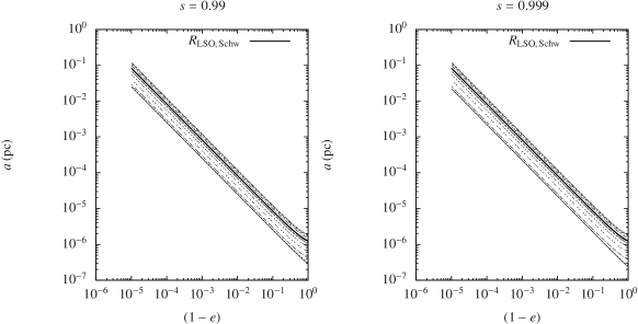
Figure 2: As in figure 1 but for a spin of $s=0.99$ (left) and $s=0.999$ (right panel). The larger the spin, the “further away” the Kerr LSO gets from the Schwarzschild LSO.

5 Number of cycles

The second type of relativistic computations that we have performed concerns the estimation of the number of cycles that certain EMRI orbital configurations that were thought to be plunging orbits (or orbits with no sufficient cycles) in the case of non-spinning MBHs can spend in a frequency regime of $f\in[10^{-4},1]$ Hz during their last year(s) of inspiral before plunging into the MBH. This is important to assess how many of these EMRIs will have sufficient Signal-to-Noise Ratio (SNR) to be detectable. The way in which these estimations have been done is the following. We start with a certain orbital configuration characterized by the orbital parameters $(p_{(0)},e_{(0)},\iota_{(0)})$. Equivalently, we can characterise the initial orbital configuration by the constant of motions $(E_{(0)},L_{z(0)},C_{(0)})$. Hence, the idea is to track the inspiral without actually integrating the equations of geodesic motion of section 3 or any other type of equations that follow the trajectory. Instead, we picture the inspiral as a sequence of geodesic orbits, each of them characterized by orbital parameters $(p_{(i)},e_{(i)},\iota_{(i)})$ (or equivalently, constants of motion $(E_{(i)},L_{z(i)},C_{(i)})$) with $i=0,\ldots,N_{\rm plunge}$, being $N_{\rm plunge}$ the final plunging configuration. The transition between each orbital configuration is governed by the GW emission. Our particular algorithm to follow the inspiral goes as follows (our implementation uses the formulæ in the appendices of Sopuerta & Yunes 2011 and the formulae derived by Gair & Glampedakis 2006):

1. Given an orbital configuration $(p_{(i)},e_{(i)},\iota_{(i)})$ and its associated constants of motion $(E_{(i)},L_{z(i)},C_{(i)})$, we compute the averaged evolution of the constants of motion, $(\dot{E},\dot{L}_{z},\dot{C})$, using the formulæ of (Gair & Glampedakis 2006), which combine post-Newtonian calculations at the 2PN order with fits to results for the GW emission based on the Teukolsky formalism (Teukolsky 1973) (for details see Hughes (2000, 2001); Glampedakis et al. (2002); Drasco & Hughes (2006); Hughes et al. (2005)).

2. For the given orbital parameters we estimate the radial period $T_{r}$, that is the time to go from apoapsis to periapsis and back to apoapsis (see Schmidt 2002; Fujita & Hikida 2009 for details of this computation. In Fujita & Hikida 2009 there is a typo in one of the relevant formulae for our computations fixed in the appendices of Sopuerta & Yunes 2011).

3. We compute the change in the constants of motion. To that end, due to the fact that the GW emission by an EMRI is relatively weak, we do not consider in general just one passage through periapsis, but several of them, say $N^{\rm peri}_{(i)}$. Thus, the change in the constants of motion is:

   $$(\Delta E_{(i)},\Delta L_{z(i)},\Delta C_{(i)}) =(\dot{E}_{(i)},\dot{L}_{z(i)},\dot{C}_{(i)})$$

   $$\times N^{\rm peri}_{(i)}\times T_{r}.$$ (15)

   And from here,

   $$(E_{(i+1)},L_{z(i+1)},C_{(i+1)}) =(E_{(i)},L_{z(i)},C_{(i)})+$$

   $$(\Delta E_{(i)},\Delta L_{z(i)},\Delta C_{(i)}).$$ (16)

4. From these new constants of motion and using similar techniques to the ones described above for the LSO computation we can find the new orbital parameters $(p_{(i+1)},e_{(i+1)},\iota_{(i+1)})$. We then go back to the first step and follow the inspiral until we detect that the new configuration corresponds to an unstable orbit corresponding to the plunge. We estimate the number of cycles as the number of times that the stellar object turned around the spin axis, $N^{\,\rm cycles}_{\varphi}$.

In Table 1 we show some results for a series of inspirals whose initial orbital parameters are such that the pair $(e,p)$ lies on the separatrix between stable and unstable orbits in the case of non-spinning MBHs (i.e. $p=6+2e$). Therefore, these are inspirals that under the assumption that spin can be neglected would have no cycles in the eLISA band. However, we can see from the values for the number of cycles in the table that many of those systems actually perform a significant number of cycles, more than sufficient to be detectable with good SNR. The number of cycles has been associated with $N_{\varphi}$ (the number of times that the azimuthal angle $\varphi$ advances $2\pi$) which is usual for binary systems. However, as we have discussed above the structure of the waveforms from EMRIs is quite rich since they contain harmonics of three different frequencies. Therefore the waveforms have cycles associated with the three frequencies $(f_{r},f_{\theta},f_{\varphi})$ which makes them quite complex and in principle this is good for detectability (assuming we have the correct waveform templates). Another fact that is worth mentioning is that the cycles quoted in Table 1 happen just before plunge and take place in the strong field region very near the MBH horizon. Then, these cycles should contribute more to the SNR than cycles taking place farther away from the MBH horizon. Regarding the accuracy of these estimations, the main sources of error are the approximations made for the radiation-reaction effects, which are based on a post-Newtonian expansions and fits to results from black hole perturbation theory. Corrections from higher-order terms will introduce corrections to these results that depend on the EMRI configuration, but those corrections should not affect the magnitude of these numbers. In the Table we quote the integers that are closer to the numerical result.

MBH mass	MBH Spin	Semimajor axis	Eccentricity	Inclination	Time to plunge	Time in band	Cycles in band
$M_{\bullet}\;(M_{\odot})$	$s$	$a_{(0)}$ (pc)	$1-e_{(0)}$	$\iota_{(0)}$ (rad)	$T_{\rm plunge}$ (yrs)	$T_{\rm band}$ (yrs)	$N_{\varphi}$
$5.0\cdot 10^{4}$	$0.30$	$9.57\cdot 10^{-3}$	$10^{-6}$	$0.00$	$3.92\cdot 10^{2}$	$0.06$	$914$
$5.0\cdot 10^{4}$	$0.30$	$9.57\cdot 10^{-3}$	$10^{-6}$	$0.70$	$3.92\cdot 10^{2}$	$0.06$	$625$
$5.0\cdot 10^{4}$	$0.90$	$9.57\cdot 10^{-3}$	$10^{-6}$	$0.00$	$3.92\cdot 10^{2}$	$0.11$	$4174$
$5.0\cdot 10^{4}$	$0.90$	$9.57\cdot 10^{-3}$	$10^{-6}$	$1.00$	$3.92\cdot 10^{2}$	$0.08$	$2646$
$1.0\cdot 10^{5}$	$0.70$	$1.91\cdot 10^{-2}$	$10^{-6}$	$0.00$	$7.87\cdot 10^{2}$	$0.29$	$6968$
$1.0\cdot 10^{5}$	$0.70$	$1.91\cdot 10^{-2}$	$10^{-6}$	$1.00$	$7.86\cdot 10^{2}$	$0.23$	$3411$
$1.0\cdot 10^{5}$	$0.99$	$1.91\cdot 10^{-2}$	$10^{-6}$	$0.00$	$4.70\cdot 10^{3}$	$0.38$	$8938$
$1.0\cdot 10^{5}$	$0.99$	$1.91\cdot 10^{-2}$	$10^{-6}$	$0.70$	$3.92\cdot 10^{3}$	$0.32$	$7892$
$5.0\cdot 10^{5}$	$0.30$	$9.57\cdot 10^{-2}$	$10^{-6}$	$0.00$	$4.31\cdot 10^{4}$	$1.98$	$8246$
$5.0\cdot 10^{5}$	$0.30$	$9.57\cdot 10^{-2}$	$10^{-6}$	$1.00$	$4.31\cdot 10^{4}$	$1.61$	$3061$
$5.0\cdot 10^{5}$	$0.95$	$9.57\cdot 10^{-2}$	$10^{-6}$	$0.00$	$5.10\cdot 10^{4}$	$2.00$	$40093$
$5.0\cdot 10^{5}$	$0.95$	$9.57\cdot 10^{-2}$	$10^{-6}$	$1.00$	$4.31\cdot 10^{4}$	$2.00$	$27600$
$1.0\cdot 10^{6}$	$0.30$	$1.91\cdot 10^{-2}$	$10^{-5}$	$0.00$	$1.27\cdot 10^{4}$	$1.98$	$10943$
$1.0\cdot 10^{6}$	$0.30$	$1.91\cdot 10^{-2}$	$10^{-5}$	$1.00$	$1.19\cdot 10^{4}$	$1.91$	$3552$
$1.0\cdot 10^{6}$	$0.70$	$1.91\cdot 10^{-2}$	$10^{-5}$	$0.00$	$1.35\cdot 10^{4}$	$1.99$	$51308$
$1.0\cdot 10^{6}$	$0.70$	$1.91\cdot 10^{-2}$	$10^{-5}$	$1.00$	$1.20\cdot 10^{4}$	$1.99$	$23291$
$1.0\cdot 10^{6}$	$0.90$	$1.91\cdot 10^{-2}$	$10^{-5}$	$0.00$	$1.40\cdot 10^{4}$	$1.99$	$58841$
$1.0\cdot 10^{6}$	$0.90$	$1.91\cdot 10^{-2}$	$10^{-5}$	$1.00$	$1.17\cdot 10^{4}$	$2.00$	$38245$
$1.0\cdot 10^{6}$	$0.99$	$1.91\cdot 10^{-2}$	$10^{-5}$	$0.00$	$1.43\cdot 10^{4}$	$2.00$	$61726$
$1.0\cdot 10^{6}$	$0.99$	$1.91\cdot 10^{-2}$	$10^{-5}$	$1.00$	$1.17\cdot 10^{4}$	$2.00$	$47678$
$5.0\cdot 10^{6}$	$0.30$	$9.57\cdot 10^{-2}$	$10^{-5}$	$0.00$	$1.44\cdot 10^{5}$	$1.93$	$5258$
$5.0\cdot 10^{6}$	$0.30$	$9.57\cdot 10^{-2}$	$10^{-5}$	$1.00$	$1.36\cdot 10^{5}$	$0.00$	$0$
$5.0\cdot 10^{6}$	$0.70$	$9.57\cdot 10^{-2}$	$10^{-5}$	$0.00$	$1.55\cdot 10^{5}$	$2.00$	$40687$
$5.0\cdot 10^{6}$	$0.70$	$9.57\cdot 10^{-2}$	$10^{-5}$	$1.00$	$1.36\cdot 10^{5}$	$2.00$	$14936$
$5.0\cdot 10^{6}$	$0.90$	$9.57\cdot 10^{-2}$	$10^{-5}$	$0.00$	$1.61\cdot 10^{5}$	$2.00$	$41369$
$5.0\cdot 10^{6}$	$0.90$	$9.57\cdot 10^{-2}$	$10^{-5}$	$1.00$	$1.35\cdot 10^{5}$	$1.99$	$30695$
$1.0\cdot 10^{7}$	$0.30$	$1.91$	$10^{-6}$	$0.00$	$4.02\cdot 10^{6}$	$1.99$	$3089$
$1.0\cdot 10^{7}$	$0.30$	$1.91$	$10^{-6}$	$1.00$	$3.78\cdot 10^{6}$	$0.00$	$0$
$1.0\cdot 10^{7}$	$0.70$	$1.91$	$10^{-6}$	$0.00$	$4.27\cdot 10^{6}$	$2.00$	$23425$
$1.0\cdot 10^{7}$	$0.70$	$1.91$	$10^{-6}$	$1.00$	$3.79\cdot 10^{6}$	$1.98$	$8747$
$1.0\cdot 10^{7}$	$0.99$	$1.91\cdot 10^{-1}$	$10^{-5}$	$0.00$	$1.44\cdot 10^{6}$	$1.98$	$22455$
$1.0\cdot 10^{7}$	$0.99$	$1.91\cdot 10^{-1}$	$10^{-5}$	$1.00$	$1.18\cdot 10^{6}$	$1.99$	$28589$
$5.0\cdot 10^{7}$	$0.30$	$9.57\cdot 10^{-1}$	$10^{-5}$	$0.00$	$1.44\cdot 10^{7}$	$0.00$	$0$
$5.0\cdot 10^{7}$	$0.30$	$9.57\cdot 10^{-1}$	$10^{-5}$	$1.00$	$1.36\cdot 10^{7}$	$0.00$	$0$
$5.0\cdot 10^{7}$	$0.70$	$9.57\cdot 10^{-1}$	$10^{-5}$	$0.00$	$1.55\cdot 10^{7}$	$1.72$	$4247$
$5.0\cdot 10^{7}$	$0.70$	$9.57\cdot 10^{-1}$	$10^{-5}$	$1.00$	$1.35\cdot 10^{7}$	$0.00$	$0$
$5.0\cdot 10^{7}$	$0.99$	$9.57\cdot 10^{-1}$	$10^{-5}$	$0.00$	$1.65\cdot 10^{7}$	$1.88$	$4422$
$5.0\cdot 10^{7}$	$0.99$	$9.57\cdot 10^{-1}$	$10^{-5}$	$1.00$	$1.35\cdot 10^{7}$	$1.52$	$4625$

Table 1: This table shows the main properties of some (prograde) inspirals that initially lie on the separatrix (LSO) of non-spinning MBHs and hence they would not be detectable in the eLISA band. The numbers in the first five columns have been already introduced in the text. The sixth column gives the time it takes for each inspiral to get to plunge. The seventh column shows how much time it spends in band assuming the plunge occurs at the end of the eLISA mission time (assumed to be $2\,$ yrs here). The last column show the number of orbital cycles in band (during $T_{\rm band}$), defined as the number of times that the azimuthal angle $\varphi$ advances $2\pi$ during the last two years before plunge. The number of GW cycles can be then defined as twice this number.

6 Impact on event rates

Only a certain fraction of stars in phase space will come close enough to interact with the MBH. These stars are said to belong to the “loss-cone” (see e.g. Frank & Rees 1976; Amaro-Seoane & Spurzem 2001).

For radii larger than $0.01$ pc the main leading mechanism for producing EMRIs is two-body relaxation (Hopman & Alexander 2005; Amaro-Seoane et al. 2007; Amaro-Seoane 2012), and this is the region of phase-space in which our analysis is applied with priority, since for a Schwarzschild MBH one has just direct plunges. For radii below $0.01$ pc we note that the enhancement in the EMRI event rate due to resonant relaxation predicted by Hopman & Alexander (2005) is severely affected by the presence of a blockade in the rate at which orbital angular momenta change takes place. This so-called “Schwarzschild barrier” is a result of the impact of relativistic precession on to the stellar potential torques, as recently shown by Merritt et al. (2011) with a few direct-summation $N-$body simulations expanded with a statistical Monte-Carlo study. Indeed, this “Schwarzschild barrier” has been corroborated in an independent work with a statistical study based on a sample of some 2,500 direct-summation $N-$body simulations by Brem et al. (2012) in which the authors include post-Newtonian corrections and also, for the first time, the implementation of a solver of geodesic equations in the same code. This barrier poses a real problem for the production of low-eccentricity EMRIs. However, high-eccentricity EMRIs, which had been classified until now wrongly of “plunges” do not have this problem, since they are a product of pure two-body relaxation. This is why we will only focus on two-body relaxation for the estimation of the rates.

The event rate can be hence approximately calculated as

$$\dot{N}_{\rm EMRI}\simeq\int^{a_{\rm EMRI}}_{0}\frac{dN_{\bullet}(a)}{\ln{\left(\theta_{\rm LC}^{-2}\right)}\,t_{r}(a)}\,,$$ (17)

with $\theta_{\rm LC}$ the loss-cone angle, $N_{\bullet}(a)$ the number of stellar black holes (SBHs) within a semi-major axis $a$ and $a_{\rm EMRI}$ a maximum radius within which we estimate the event rate $\dot{N}_{\rm EMRI}$. We assume that the SBHs distribute around the central MBH following a power-law cusp of exponent $\gamma$, i.e. that the density profile follows $\rho\propto r^{-\gamma}$ within the region where the gravity of the MBH dominates the gravity of the stars, with $\gamma$ ranging between 1.75 and 2 for the heavy stellar components (Peebles 1972; Bahcall & Wolf 1976, 1977; Amaro-Seoane et al. 2004; Preto et al. 2004; Alexander & Hopman 2009; Preto & Amaro-Seoane 2010; Amaro-Seoane & Preto 2011) and see Gurevich (1964) for an interesting first idea of this concept. We then have that the number of stars within a radius $r$ is

$$n(r)=\frac{\left(3-\gamma\right)}{4\,\pi}\left(\frac{M_{\bullet}}{m_{\star}}\right)\left(\frac{1}{R_{\rm infl}^{3}}\right)\left(\frac{r}{R_{\rm infl}}\right)^{-\gamma}\,.$$ (18)

Hence, the number of SBHs within $a$ is

$$N_{\bullet}(a)\simeq N_{0}\left(\frac{a}{R_{0}}\right)^{3-\gamma}\,.$$ (19)

Hence, we have that

$$dN_{\bullet}(a)=(3-\gamma)\frac{N_{0}}{R_{0}}\left(\frac{a}{R_{0}}\right)^{2-\gamma}da\,.$$ (20)

6.1 The Schwarzschild case

We know that (see e.g. Alexander & Livio 2001; Amaro-Seoane & Spurzem 2001) $\theta^{-2}_{\rm LC}\simeq J_{\rm max}/J_{\rm LC}$. Since the loss-cone angular momentum can be approximated as $J_{\rm LC}\simeq 4\,GM_{\bullet}/c$ and $J_{\rm max}=\sqrt{GM_{\bullet}a}$, we have that

$$\theta^{-2}_{\rm LC}\simeq\sqrt{\frac{a}{8\,R_{\rm Schw}}},$$ (21)

We assume also that relaxation is dominated by a single stellar black hole (SBH) population, since because of mass segregation the most massive objects sink down to the centre and the light stars are pushed out from the centre. The relaxation time at a distance $a$ is

$$t_{r}(a)=t_{0}\left(\frac{a}{R_{0}}\right)^{\gamma-3/2}\,,$$ (22)

with

$$t_{0}=0.3389\,\frac{\sigma_{0}^{3}}{\ln\Lambda\,G^{2}m_{\bullet}^{2}\,n_{0}}\,.$$ (23)

Since (see e.g. Amaro-Seoane et al. 2007)

$$n_{0} =\frac{3-\gamma}{4\pi}{N_{0}}{R_{0}^{3}}$$ (24)

$$\sigma_{0}^{2} =\frac{1}{1+\gamma}\frac{GM_{\bullet}}{R_{0}},$$ (25)

we have that equation (23) becomes

$$t_{0}\simeq 4.26\,\frac{1}{(3-\gamma)(1+\gamma)^{3/2}}\frac{\sqrt{R_{0}^{3}(GM_{\bullet})^{-1}}}{\ln\Lambda\,N_{0}}\left(\frac{M_{\bullet}}{m_{\bullet}}\right)^{2}\,.$$ (26)

We now define a critical radius at which the two regimes that lead the evolution of the EMRI decouple. The first evolution is dominated by relaxational processes, via exchange of $E$ and $J$ between SBHs on a capture orbit with stars from the surrounding stellar system, while in the second regime the evolution of the EMRI is totally dominated by the emission of gravitational waves. This is given in figure 1 of Amaro-Seoane et al. (2007) with their red curve. In other words, the line gives us the radius as a function of $a$ at which the relaxational time at periapsis is approximately equal to the timescale defined by the approximation of Peters (1964). Hence, we have to solve

$$t_{\rm r}(a)(1-e) =K\,t_{\rm GW}(a,\,e)$$

$$J(a,\,e) =J_{\rm LC}$$

$$(1-e)\,a =\frac{8\,G{\cal M}_{\bullet}}{c^{2}}$$ (27)

In the first equality, $K$ is a factor of order unity. In the last equality we assume a Schwarzschild radius and we assume that the LSO is at $4\times\,R_{\rm Schw}$ Approximating $e\sim 1$, the function $f(e)$ from Peters (1964) $f(e)=425/(768\,\sqrt{2})$. Hence

$$t_{\rm GW}(a,\,e)\cong\sqrt{2}\,\frac{24}{85}\frac{c^{5}}{G^{3}}\frac{a^{4}}{M_{\bullet}^{2}\,m_{\bullet}}\left(1-e\right)^{7/2}\,.$$ (28)

And so, finally from equations (27), (22) and (26) and solving for $a_{\rm EMRI}$, we have that

$$a_{\rm EMRI}\simeq R_{0}\left[16.97\,K\,\left(3-\gamma\right)\left(1+\gamma\right)^{3/2}\ln\Lambda\,N_{\bullet}\frac{m_{\bullet}}{M_{\bullet}}\right]^{\frac{1}{\gamma-3}}\,.$$ (29)

Or, absorbing some constants into a newly defined $K_{\gamma}$,

$$a_{\rm EMRI} =K_{\gamma}\,R_{0}\,\left(\frac{1}{\ln\Lambda}\,\frac{M_{\bullet}}{N_{\bullet}\,m_{\bullet}}\right)^{\frac{1}{3-\gamma}}$$

$$K_{\gamma} :=\left[16.97\,K\,\left(3-\gamma\right)\left(1+\gamma\right)^{3/2}\right]\,.$$ (30)

We can then derive the event rate for the Schwarzschild case, based on 17,

$$\dot{N}_{\rm EMRI}^{\rm Schw} \cong 0.235\,\frac{4\,\left(3-\gamma\right)^{2}\left(1+\gamma\right)^{3/2}}{9-4\gamma}\,K_{\gamma}^{\frac{9-4\gamma}{2}}$$

$$\frac{\ln\Lambda^{\frac{2\gamma-3}{6-2\gamma}}}{\ln\left(\frac{a_{\rm EMRI}}{8\,R_{\rm Schw}}\right)}\,\left(\frac{N_{\bullet}m_{\bullet}}{M_{\bullet}}\right)^{\frac{3}{6-2\gamma}}\sqrt{\frac{GM_{\bullet}}{R_{0}^{3}}}\,.$$ (31)

The last equation is based on the assumption that equation (27) holds, and the last equality, $(1-e)a=8\,GM_{\bullet}/c^{2}$, is the “effective” value of the periapsis for the last parabolic stable orbit (LSO from now onwards) for a Schwarzschild MBH. I.e. if the star is on an orbit that in Newtonian dynamics leads to a periapsis smaller than this value, the star disappears if we take into account relativistic dynamics.

6.2 The Kerr case

In the Kerr case we simply have to recalculate where this LSO is by taking into account the value of the spin of the MBH. We then have to either shrink or enlarge it by a certain factor function of the inclination and spin, ${\cal W}(\iota,\,s)$, so that the effective pericentre of LSO is

$$(1-e)\,a={\cal W}(\iota,\,s)\times\frac{8\,GM_{\bullet}}{c^{2}}\,.$$ (32)

This quantity can be derived from the separatrices of the figures in section 3. If the orbit can get closer to the MBH in the Kerr case, then ${\cal W}(\iota,\,s)<1$; otherwise ${\cal W}(\iota,\,s)>1$. Since the separatrices are nearly parallel, we hence can define ${\cal W}(\iota,\,s)$ like

$${\cal W}(\iota,\,s):=\left\langle\frac{a_{\rm LSO,\,Kerr}}{a_{\rm LSO,\,Schw}}\right\rangle=\frac{1}{N}\,\sum_{i}\frac{a_{\rm LSO,\,Kerr}(e_{i})}{a_{\rm LSO,\,Schw}(e_{i})}\,.$$ (33)

That is, given a spin and an inclination, we take for $N$ values of the eccentricity the semimajor axis corresponding to the Kerr value, $a_{\rm LSO,\,Kerr}(e)$ and to the Schwarzschild case, $a_{\rm LSO,\,Schw}$ and we sum for the ratio of the two semi-majors over all eccentricities. This allows us to calculate by how much the LSO has been “shifted”.

Spin ($s$)	Inclination ($\iota$, rad)	${\cal W}(\iota,\,s)$
0.900	0.100	0.429452
0.900	0.400	0.448093
0.900	0.700	0.499450
0.900	1.000	0.598278
0.900	1.300	0.739339
0.900	1.570	0.883679
0.900	-0.100	1.415955
0.900	-0.400	1.377239
0.900	-0.700	1.295011
0.900	-1.000	1.175760
0.950	0.100	0.370036
0.950	0.400	0.386009
0.950	0.700	0.436921
0.950	1.000	0.548352
0.950	1.300	0.708257
0.950	1.570	0.867320
0.950	-0.400	1.396449
0.950	-0.700	1.309052
0.950	-1.000	1.181942
0.950	-1.300	1.024866
0.990	0.100	0.297301
0.990	0.400	0.306924
0.990	0.700	0.354716
0.990	1.000	0.494738
0.990	1.300	0.679468
0.990	1.570	0.852821
0.990	-0.100	1.454732
0.990	-0.400	1.411720
0.990	-0.700	1.320145
0.990	-1.000	1.186631
0.990	-1.300	1.020814
0.999	0.100	0.260205
0.999	0.400	0.264063
0.999	0.700	0.310302
0.999	1.000	0.479038
0.999	1.300	0.672349
0.999	1.570	0.849364
0.999	-0.100	1.458589
0.999	-0.400	1.415145
0.999	-0.700	1.322624
0.999	-1.000	1.187655
0.999	-1.300	1.019828

Table 2: Values for ${\cal W}$.

If we redo the derivation of (31) taking into account equation 32, we can obtain $\dot{N}_{\rm EMRI}$ in function of ${\cal W}$, $\dot{N}_{\rm EMRI}^{\rm Kerr}$ and, hence, we can calculate the ratio of the rates as a function of the inclination $\iota$ and spin $s$:

$${{a}_{\rm EMRI}^{\rm Kerr}} ={{a}_{\rm EMRI}^{\rm Schw}}\times{\cal W}^{\frac{-5}{6-2\gamma}}(\iota,\,s)$$ (34)

$${\dot{N}_{\rm EMRI}^{\rm Kerr}} ={\dot{N}_{\rm EMRI}^{\rm Schw}}\times{\cal W}^{\frac{20\gamma-45}{12-4\gamma}}(\iota,\,s)\,.$$ (35)

For instance, for a spin of $s=0.999$ and an inclination of $\iota=0.4\,$rad, we estimate that ${\cal W}\sim 0.26$ and, thus, $\dot{N}_{\rm EMRI}^{\rm Kerr}\sim 30$. I.e. we boost the event rates by a factor of 30 in comparison to a non-rotating MBH.

7 Net effect of resonant relaxation on EMRI rates

7.1 The role of vectorial resonant relaxation

To understand the impact of the previous calculation on event rates for EMRIs we have to elaborate on prograde and retrograde orbits. We have seen that retrograde EMRI orbits see the central MBH as an effectively “larger” MBH; i.e. it is easier to plunge through the horizon. Contrary, prograde EMRI orbits “see” the effective size of the MBH shrink and, thus, have a harder time in hitting the central MBH. It is therefore important to assess the orientation of orbits in the regime of interest. It takes on average (vectorial) resonant relaxation (RR) a time $t_{\rm RR,\,v}$ to rotate coherently the orbital plane of an orbit by an angle $\pi/2$ (Hopman & Alexander 2006). To change a prograde (retrograde) orbit to a retrograde (prograde) orbit, it takes four times longer: The $\pi/2$ rotation is the maximum that can be obtained over the self-quenching time; the rest to get up to a full $\pi$ rotation is done non-coherently over 4 coherence times (see Bregman & Alexander 2011, for a discussion of the numeric prefactors).

It should be noted that vector RR is invariant under precession (see e.g. Hopman & Alexander 2006). We must note also that the change in the inclination of the orbit with respect to the spin axis due to GW emission is relatively rather small (see Hughes (2000, 2001)), so small that frequently it has been assumed to be constant, which provides an extra equation for the evolution of the Carter constant in the inspiral process, making things significantly simpler.

The dependence of the transverse RR torque (i.e. direction-changing torque) on the eccentricity has been measured from simulations by Gürkan & Hopman (2007). In their work, the authors derive that it grows quadratically by a factor $3$ in total from $0$ to $1$.

The radius of the sphere of influence is

$$r_{\rm infl}=\frac{1}{1+\gamma}\frac{GM_{\bullet}}{\sigma_{0}^{2}}\approx 1~{}{\rm pc}\frac{1}{1+\gamma}\left(\frac{M_{\bullet}}{10^{6}\,M_{\odot}}\right)\left(\frac{60~{}{\rm km/s}}{\sigma_{0}}\right)^{2}\,,$$ (36)

for a given exponent $\gamma$. Within this radius the relaxation time is

$$t_{\rm r}(r) \propto\left(1+\gamma\right)^{-3/2}\frac{\ln\Lambda\,\sigma^{3}(r)}{G^{2}\langle m\rangle m_{\rm CO}n(r)}$$

$$\simeq 2\times 10^{8}\,{\rm yr}\left(1+\gamma\right)^{-3/2}\left(\frac{\sigma}{100\,\mathrm{km\,s}^{-1}}\right)^{3}\left(\frac{10\,M_{\odot}}{m_{\rm CO}}\right)$$

$$\left(\frac{10^{6}\,M_{\odot}{\rm pc}^{-3}}{\langle m\rangle n}\right)\,.$$ (37)

In this equation we follow the usual notation: $\sigma(r)$ is the local velocity dispersion; for $r<r_{\rm infl}$ it is approximately the Keplerian orbital speed $\sqrt{GM_{\bullet}r^{-1}}$; $n(r)$ is the local density of stars, $\langle m\rangle$ is the average stellar mass, $m_{\rm CO}$ is the individual mass of the compact object, which we assume to be all SBHs, and take a mass of $m_{\rm CO}=10\,M_{\odot}$ for all of them. In the vicinity of a MBH, ($r<r_{\rm infl}$), $\Lambda\approx M_{\bullet}/m_{\star}$ (Bahcall & Wolf 1976; Lightman & Shapiro 1977), and typically $\ln\Lambda\sim 11$.

Relaxation redistributes orbital energy amongst stellar-mass objects until SBHs form a power-law density cusp, $n(r)\propto r^{-\gamma}$ with $\gamma\simeq 1.75$ around the MBH, while less massive species arrange themselves into a shallower profile, with $\alpha\simeq 1.4-1.5$ as we have mentioned earlier, although recent studies have found a general solution to the problem of mass segregation around MBH in galactic nuclei, with a more efficient diffusion for the heavy stars, reaching a $\gamma\sim-2$ in the “strong mass-segregation” regime (Alexander & Hopman 2009; Preto & Amaro-Seoane 2010; Amaro-Seoane & Preto 2011).

Since $\sigma(r)^{2}=GM_{\bullet}/r$ and we take that $\langle m\rangle=0.7\,M_{\odot}$ and, as mentioned, $m_{\rm CO}=10\,M_{\odot}$, we have all information to derive $t_{\rm r,\,peri}(r):=(1-e)\,t_{\rm r}$ from Equation (37) and (18).

As regards the explicit expression for the characteristic timescale for vectorial resonant relaxation, from Hopman & Alexander (2006) we have that

$$t_{\rm RR,\,v}=P(a)\frac{M_{\bullet}}{m_{\star}}\frac{\beta_{v}(e)^{2}}{\sqrt{N(a)}}\,,$$ (38)

where we have taken into account the corrections for high values of $e$ as given in Gürkan & Hopman (2007), $\beta_{v}(e)=0.28\,(e^{2}+0.5)$ and $P(a)=a^{3/2}/(GM_{\bullet})^{1/2}$. This allows us to follow the dependence with the radius (and eccentricity) of the ratio $t_{\rm r,\,peri}/t_{\rm RR,\,v}$.

If we now equate the timescales of interest, the gravitational radiation driven time $t_{\rm GW}$, defined as in the approximation of Peters (1964), to the two-body relaxation time at periapsis, $t_{\rm r,\,peri}$, we obtain the short-dashed curve of figure 3 on the left of this line, the contribution of GW radiation to orbital evolution dominates over two-body relaxation. In the absence of resonant relaxation, if a SBH crosses this line from the right (lower eccentricities), it will become an EMRI, provided, of course, that it is still on a stable orbit, i.e. above the separatrix corresponding to its orbital orientation. For a Schwarzschild MBH, all separatrices are the same and there is a unique critical point (PS). A SBH with a semi-major axis larger that the value at PS will experience a direct plunge if relaxation brings its eccentricity to a high value because it will cross the separatrix (and be swallowed in less than an orbital time) before it has a chance to enter into the GW-dominated regime. Conversely, objects with smaller semi-major axis values are much more likely to end up as EMRIs rather than plunges.

Figure 3: Left panel: Relation between different timescales in the $s=0.999$ case. As in the prior section, we display the Schwarzschild separatrix as a solid, black line and the separatrices for different inclinations with different curves in light grey. The dashed, blue line shows the value of $a$ and $1-e$ for which the vectorial resonant relaxation timescale ($t_{\rm RR,\,v}$) is equal to the gravitational loss timescale ($t_{\rm GW}$). The dashed, dotted line corresponds to the values of $a$ and $1-e$ for which the relaxation time at periapsis ($t_{\rm r,\,peri}$) equals the gravitational loss timescale. Right panel: Same as the left panel but zoomed to see where the dashed, red curve intersects the last one of the retrograde, Schwarzschild and prograde separatrices. We show this with a blue dot and a long-dashed curve for the retrograde case which yields the last separatrix, with a green dot and a green, short-dashed curve for the Schwarzschild separatrix and with a red dot and a dash-dotted curve for the last separatrix of the prograde case. These lines give us $a_{\rm EMRI,\,retro}$, $a_{\rm EMRI,\,Schw}$ and $a_{\rm EMRI,\,pro}$, correspondingly.

For a fast spinning SMBH, the separatrix for prograde orbits is shifted to significantly lower $a$ values, with a corresponding higher value of the critical semi-major axis, corresponding to the point PP in figure 3. As we have explained above, it is this effect which can lead to a significant increase in the EMRI rate, combined with the fact that the critical point for retrograde orbits (PR) is much less affected and that an isotropic orbit distribution is expected, thanks to relaxational processes. However this increase in EMRI rate would can be thwarted by vector RR if this process can change the orbital orientation of a SBH after it has crossed the “$t_{\rm GW}=t_{\rm r,\,peri}$” line and before it has completed its GW-driven inspiral, i.e. on a timescale shorter than $t_{\rm GW}$. Indeed, if the orbit becomes significantly less prograde as the the inspiral takes place, due to RR, the separatrix moves up and the SBH might suddenly find itself on a plunge orbit.

To check for this possibility, we also plot, in figure 3, a long-dashed line corresponding to the condition $t_{\rm GW}=t_{\rm RR,\,v}$, with $t_{\rm GW}<t_{\rm RR,\,v}$ on the left of this line. SBHs that cross the “$t_{\rm GW}=t_{\rm r,\,peri}$” line while on the left side of the “$t_{\rm GW}=t_{\rm RR,\,v}$” line keep their orbital orientation during their inspiral and complete it without abrupt plunge. One can see that, for our choice of parameters, this is the case for all prograde orbits. On the other hand, retrograde orbits can cross the “$t_{\rm GW}=t_{\rm r,\,peri}$” line while RR is still effective enough to change their orientation during inspiral. However, the effect of RR on retrograde orbits cannot reduce significantly the total EMRI rate and may even increase it slightly because (1) these orbits contribute less that the prograde ones (and more to the plunge rate) and (2) statistically, RR is more likely to make the orbit become less retrograde which pushes down the separatrix.

Finally, we also note that for the other proposed mechanism to produce EMRIs, the tidal separation of a binary containing a compact object (Miller et al. 2005; Amaro-Seoane et al. 2007), the captured objects typically have much lower eccentricities and smaller semi-major axis. Therefore, they cross “$t_{\rm GW}=t_{\rm r,\,peri}$” line and start their inspiral, with orbital parameters well above the uppermost separatrix (for retrograde orbits). As the GW-driven trajectory in the $e-a$ plane is basically parallel to the separatrices, there is no danger of a premature plunge, even though RR has ample time to flip the orbital orientation during inspiral.

8 Conclusions

In this article we have addressed the problem of direct plunges and MBHs. If this is a Schwarzschild MBH, the compact object will plunge through the horizon and will hence not contribute to the mapping of space and time around the MBH, contrary to an EMRI, which describes thousands of cycles before it merges with the central MBH. On the other hand, the event rate of plunges is much larger than that of EMRIs, as a number of different studies by different authors using different methods find.

Up to now spin effects of the central MBH have been always ignored. Hence, the question arises, whether a plunge is really a plunge when the central MBH is spinning. This consideration has been so far always ignored.

So as to estimate EMRI event rates, one needs to know whether the orbital configuration of the compact object is stable or not, because this is the kernel of the difference between an EMRI and a plunge. In this paper we take into account the fact that the spin makes the LSO to be much closer to the horizon in the case of prograde orbits but it pushes it away for retrograde orbits. Since the modifications introduced by the spin are not symmetric with respect to the non-spinning case, and they are more dramatic for prograde orbits, we prove that the inclusion of spin increases the number of EMRI events by a significant factor. The exact factor of this enhancement depends on the spin, but the effect is already quite important for spins around $s\sim 0.7$.

We also prove that these fake plunges, “our” EMRIs, do spend enough cycles inside the band of eLISA to be detectable, i.e. they are to be envisaged as typical EMRIs. We note here that whilst it is true that EMRIs very near the new separatrix shifted by the spin effect will probably contribute not enough cycles to be detected, it is equally true for the old separatrix (Schwarzschild, without spin). In this sense, we find that the spin increases generically the number of cycles inside the band for prograde EMRIs in such a way that EMRIs very near to the non-spin separatrix, which contributed few cycles, become detectable EMRIs. In summary, spin increases the area, in configuration space of detectable EMRIs. We predict thus that EMRIs will be highly dominated by prograde orbits.

Moreover, because spin allows for stable orbits very near the horizon in the prograde case, the contribution of each cycle to the SNR is significantly bigger than each cycle of an EMRI around a non-spinning MBH.

We then show that vectorial resonant relaxation will not be efficient enough to change prograde orbits into retrogrades once GW evolution dominates (which would make the EMRIs plunge instantaneously, as they would be in a non-allowed region of phase space).

These new kind of EMRIs we describe here, high-eccentric EMRIs, are produced by two-body relaxation and, as such, they are ignorant of the Schwarschild barrier. While low-eccentricity EMRIs run into the problem of having to find a way to travers this barrier, our “plunge-EMRIs” do not. We predict that EMRI rates will be dominated by high-eccentricity binaries, with the proviso that the central MBH is Kerr.

References

- Alexander & Hopman (2003) Alexander T., Hopman C., 2003, ApJ Lett., 590, 29
- Alexander & Hopman (2009) Alexander T., Hopman C., 2009, ApJ, 697, 1861
- Alexander & Livio (2001) Alexander T., Livio M., 2001, ApJ Lett., 560, 143
- Amaro-Seoane (2004) Amaro-Seoane P., 2004, PhD thesis, PhD Thesis, Combined Faculties for the Natural Sciences and for Mathematics of the University of Heidelberg, Germany. VII + 174 pp. (2004), http://www.ub.uni-heidelberg.de/archiv/4826
- Amaro-Seoane (2012) —, 2012, ArXiv e-prints
- Amaro-Seoane et al. (2012a) Amaro-Seoane P., Aoudia S., Babak S., Binétruy P., Berti E., Bohé A., Caprini C., Colpi M., Cornish N. J., Danzmann K., Dufaux J.-F., Gair J., Jennrich O., Jetzer P., Klein A., Lang R. N., Lobo A., Littenberg T., McWilliams S. T., Nelemans G., Petiteau A., Porter E. K., Schutz B. F., Sesana A., Stebbins R., Sumner T., Vallisneri M., Vitale S., Volonteri M., Ward H., 2012a, Accepted for publication at GW Notes
- Amaro-Seoane et al. (2012b) —, 2012b, Classical and Quantum Gravity, 29, 124016
- Amaro-Seoane et al. (2004) Amaro-Seoane P., Freitag M., Spurzem R., 2004, MNRAS
- Amaro-Seoane et al. (2007) Amaro-Seoane P., Gair J. R., Freitag M., Miller M. C., Mandel I., Cutler C. J., Babak S., 2007, Classical and Quantum Gravity, 24, 113
- Amaro-Seoane & Preto (2011) Amaro-Seoane P., Preto M., 2011, Classical and Quantum Gravity, 28, 094017
- Amaro-Seoane & Spurzem (2001) Amaro-Seoane P., Spurzem R., 2001, MNRAS, 327, 995
- Bahcall & Wolf (1976) Bahcall J. N., Wolf R. A., 1976, ApJ, 209, 214
- Bahcall & Wolf (1977) —, 1977, ApJ, 216, 883
- Bardeen (1970) Bardeen J. M., 1970, Nat, 226, 64
- Baumgardt et al. (2004) Baumgardt H., Makino J., Ebisuzaki T., 2004, ApJ, 613, 1143
- Berry & Gair (2012) Berry C. P. L., Gair J. R., 2012, ArXiv e-prints
- Binney & Tremaine (1987) Binney J., Tremaine S., 1987, Galactic Dynamics. Princeton University Press
- Boyer & Lindquist (1967) Boyer R. H., Lindquist R. W., 1967, Journal of Mathematical Physics, 8, 265
- Bregman & Alexander (2011) Bregman M., Alexander T., 2011, ArXiv e-prints
- Brem et al. (2012) Brem P., Amaro-Seoane P., Sopuerta C., 2012, Submitted to MNRAS
- David et al. (1987a) David L. P., Durisen R. H., Cohn H. N., 1987a, ApJ, 313, 556
- David et al. (1987b) —, 1987b, ApJ, 316, 505
- Drasco & Hughes (2004) Drasco S., Hughes S. A., 2004, Phys. Rev. D, 69, 044015
- Drasco & Hughes (2006) —, 2006, Phys. Rev. D, 73, 024027
- Eisenhauer et al. (2005) Eisenhauer F., Genzel R., Alexander T., Abuter R., Paumard T., Ott T., Gilbert A., Gillessen S., Horrobin M., Trippe S., Bonnet H., Dumas C., Hubin N., Kaufer A., Kissler-Patig M., Monnet G., Ströbele S., Szeifert T., Eckart A., Schödel R., Zucker S., 2005, ApJ, 628, 246
- Erwin et al. (2004) Erwin P., Graham A. W., Caon N., 2004, in Coevolution of Black Holes and Galaxies, L. C. Ho, ed.
- Ferrarese & Ford (2005) Ferrarese L., Ford H., 2005, Supermassive Black Holes in Galactic Nuclei: Past, Present and Future Research
- Frank & Rees (1976) Frank J., Rees M. J., 1976, MNRAS, 176, 633
- Freitag et al. (2006) Freitag M., Amaro-Seoane P., Kalogera V., 2006, ApJ, 649, 91
- Freitag & Benz (2002) Freitag M., Benz W., 2002, A&A, 394, 345
- Fujita & Hikida (2009) Fujita R., Hikida W., 2009, Classical and Quantum Gravity, 26, 135002
- Gair & Glampedakis (2006) Gair J. R., Glampedakis K., 2006, Ph. Rev. D, 73, 064037
- Ghez et al. (2005) Ghez A. M., Salim S., Hornstein S. D., Tanner A., Lu J. R., Morris M., Becklin E. E., Duchêne G., 2005, ApJ, 620, 744
- Ghez et al. (2008) Ghez A. M., Salim S., Weinberg N. N., Lu J. R., Do T., Dunn J. K., Matthews K., Morris M. R., Yelda S., Becklin E. E., Kremenek T., Milosavljevic M., Naiman J., 2008, ApJ, 689, 1044
- Gillessen et al. (2009) Gillessen S., Eisenhauer F., Trippe S., Alexander T., Genzel R., Martins F., Ott T., 2009, ApJ, 692, 1075
- Glampedakis et al. (2002) Glampedakis K., Hughes S. A., Kennefick D., 2002, Phys. Rev. D, 66, 064005
- Gurevich (1964) Gurevich A., 1964, Geomag. Aeronom., 4, 247
- Gürkan & Hopman (2007) Gürkan M. A., Hopman C., 2007, MNRAS, 379, 1083
- Häring & Rix (2004) Häring N., Rix H.-W., 2004, ApJ Lett., 604, L89
- Hopman & Alexander (2005) Hopman C., Alexander T., 2005, ApJ, 629, 362
- Hopman & Alexander (2006) —, 2006, ApJ, 645, 1152
- Hopman et al. (2007) Hopman C., Freitag M., Larson S. L., 2007, MNRAS, 378, 129
- Hughes (2000) Hughes S. A., 2000, Ph. Rev. D, 61, 084004
- Hughes (2001) —, 2001, Ph. Rev. D, 64, 064004
- Hughes et al. (2005) Hughes S. A., Drasco S., Flanagan É. É., Franklin J., 2005, Physical Review Letters, 94, 221101
- Khalisi et al. (2007) Khalisi E., Amaro-Seoane P., Spurzem R., 2007, MNRAS
- Kormendy (2004) Kormendy J., 2004, in Coevolution of Black Holes and Galaxies, from the Carnegie Observatories Centennial Symposia., Ho L., ed., Cambridge University Press, p. 1
- Lightman & Shapiro (1977) Lightman A. P., Shapiro S. L., 1977, ApJ, 211, 244
- Magorrian & Tremaine (1999) Magorrian J., Tremaine S., 1999, MNRAS, 309, 447
- Merritt et al. (2011) Merritt D., Alexander T., Mikkola S., Will C. M., 2011, Phys. Rev. D, 84, 044024
- Miller et al. (2005) Miller M. C., Freitag M., Hamilton D. P., Lauburg V. M., 2005, ApJ Lett., 631, L117
- Misner et al. (1973) Misner C. W., Thorne K. S., Wheeler J. A., 1973, Gravitation
- Murphy et al. (1991) Murphy B. W., Cohn H. N., Durisen R. H., 1991, ApJ, 370, 60
- Peebles (1972) Peebles P. J. E., 1972, ApJ, 178, 371
- Peters (1964) Peters P. C., 1964, Physical Review, 136, 1224
- Preto & Amaro-Seoane (2010) Preto M., Amaro-Seoane P., 2010, ApJ Lett., 708, L42
- Preto et al. (2004) Preto M., Merritt D., Spurzem R., 2004, ApJ Lett., 613, L109
- Rubbo et al. (2006) Rubbo L. J., Holley-Bockelmann K., Finn L. S., 2006, ApJ Lett., 649, L25
- Schmidt (2002) Schmidt W., 2002, Classical and Quantum Gravity, 19, 2743
- Sołtan (1982) Sołtan A., 1982, MNRAS, 200, 115
- Sopuerta & Yunes (2011) Sopuerta C. F., Yunes N., 2011, Phys. Rev. D, 84, 124060
- Syer & Ulmer (1999) Syer D., Ulmer A., 1999, MNRAS, 306, 35
- Teukolsky (1973) Teukolsky S. A., 1973, ApJ, 185, 635
- Tremaine et al. (2002) Tremaine S., Gebhardt K., Bender R., Bower G., Dressler A., Faber S. M., Filippenko A. V., Green R., Grillmair C., Ho L. C., Kormendy J., Lauer T. R., Magorrian J., Pinkney J., Richstone D., 2002, ApJ, 574, 740
- Wang & Merritt (2004) Wang J., Merritt D., 2004, ApJ, 600, 149
- Yu & Tremaine (2002) Yu Q., Tremaine S., 2002, MNRAS, 335, 965
- Yunes et al. (2008) Yunes N., Sopuerta C. F., Rubbo L. J., Holley-Bockelmann K., 2008, ApJ, 675, 604