Detection of transiting Jovian exoplanets by Gaia photometry – expected yield

Abstract

Several attempts have been made in the past to assess the expected number of exoplanetary transits that the Gaia space mission will detect. In this Letter we use the updated design of Gaia and its expected performance, and apply recent empirical statistical procedures to provide a new assessment. Depending on the extent of the follow-up effort that will be devoted, we expect Gaia to detect a few hundreds to a few thousands transiting exoplanets.

1 Introduction

Gaia is a planned European Space Agency (ESA) mission, scheduled to be launched at 2013. It will perform an all-sky astrometric and spectrophotometric survey of point-like objects between 6th and 20th magnitude. The primary goal of the telescope is to explore the formation, dynamical, chemical and star-formation evolution of the Milky Way galaxy. The main science product of Gaia will be high precision astrometry, backed with photometry and spectroscopy. It will observe about 1 billion stars, a few million galaxies, half a million quasars, and a few hundred thousands asteroids (Lindegren 2010).

Gaia will operate in a Lissajous-type orbit, around the L2 point of the Sun-Earth system, about $1.5$ million kilometers from Earth in the anti-Sun direction. It will have a dual telescope, with a common structure and common focal plane. During its five-year operational lifetime, the spacecraft will continuously spin around its axis, with a constant speed of $60\,\mathrm{arcsec\,s}^{-1}$. As a result, during a period of six hours, the two astrometric fields of view will scan all objects located along the great circle perpendicular to the spin axis. As a result of the basic angle of $106.5\arcdeg$ separating the astrometric fields of view on the sky, objects will transit the two fields of view with a delay of $106.5$ minutes. Due to the spin motion of six-hour period, and a $63$-day-period precession, the scanning law will be peculiar and irregular. This scanning law will result in a total of $70$ measurements on average for each celestial object Gaia will observe (de Bruijne 2012).

Gaia will provide photometry in several passbands, the widest of which will be a ’white’ passband dubbed $G$, centered on $\lambda_{0}=673\,\mathrm{nm}$, with a width of $\Delta\lambda=440\,\mathrm{nm}$. In what follows we use the apparent $G$ magnitude as approximately equal to the apparent $V$ magnitude. One can expect a milli-magnitude (mmag) precision in the $G$ band for most of the objects Gaia will observe, down to 14th–16th $G$ magnitude, and $10\,\mathrm{mmag}$ at the worst case of 19th magnitude objects (Jordi et al. 2010). The exact limiting magnitude for a $1\,\mathrm{mmag}$ precision depends on instrumental factors which are not yet “frozen” (de Bruijne 2012).

The $1\,\mathrm{mmag}$ precision of Gaia photometry naturally raises the question of whether it can be used to detect exoplanetary transits. While $1\,\mathrm{mmag}$ precision is nominally more than sufficient for the detection of Jovian transiting planets, the low cadence and the small number of measurements make the feasibility of this detection a non-trivial question. In the literature, there have been several conflicting estimates as to the number of transits detectable by Gaia, based on different assumptions.

Høg (2002) estimated the expected number of transit detections by Gaia at $250$, for long-period planets, with orbital radius of $0.5\,\mathrm{AU}$. According to Høg (2002), the expected yield of hot Jupiters (HJs) and very hot Jupiters (VHJs), with orbital radii of $0.1-0.01\,\mathrm{AU}$ was $6250$ and $625000$ respectively. Høg (2002) based these estimates on some general assumptions. First, the planets frequency was approximated as $\sim 1\%$, which already proved as overestimated for HJs (Beatty & Gaudi 2008, hereafter BG). Second, Høg did not account for the stellar density and its variation due to galactic structure, and neglected extinction by dust. He assumed that the number of stars Gaia will observe with $1\,\mathrm{mmag}$ precision (up to magnitude $G=15.5$) is $10^{9}$. Finally, he assumed that a transit detection can be made with only one transit observation per system, counting on Gaia astrometric observations to complement the transit observation.

Robichon (2002) performed transit simulations with the assumed Gaia photometry to estimate the number of detections, and concluded that Gaia will detect between $4000$ and $40000$ transiting Jupiter-like planets. He assumed that the number of individual observations per star would be between $100$ and $300$ with an average of $130$. He also used a galactic model (Haywood et al. 1997), and derived the probability distribution of the number of observations during transits using Gaia scanning law. We suspect that these predictions are overestimated, due to the fact that the currently planned scanning law of Gaia implies an average of $70$ measurements per star, and not $130$. We will refer to Robichon’s estimates in more detail in section 3.

In this short Letter we present a new estimate, one that we believe is more realistic than the previous ones. It is based on the methodology of BG, which includes broad assumptions about the galactic structure, as well as implicit assumptions about the geometric transit probability and the effects of stellar variability, that rely on statistics from completed transit surveys. The field of planetary transits of HJs and VHJs seems to have come to a certain maturity from which we can draw some statistical assumptions. We feel it is not yet the case for transits of smaller planets (’Saturnian’ and ’Neptunian’), and we therefore do not address these issues here.

Providing more accurate and up-to-date predictions of the number of transiting planets detectable by Gaia is important for the ongoing effort of developing the Gaia analysis pipeline. Moreover, detection of planetary transits requires considerable follow-up effort, which is also a reason for having a reliable estimate of this number. We took upon ourselves to provide a somewhat more rigorous analysis, based on empirical statistics, simply because the estimates in the literature are too varied and inconsistent. At the time they were made, the field of transit surveys was too young, and much had yet to be learned. The time has come to provide a more decisive estimate, based on the current more evolved understanding of the problem.

2 Predicting the transit yield

BG presented a statistical methodology to predict the yield of transiting planets from photometric surveys. Their method takes into consideration the frequency of short period planets, variations in the stellar density due to the galactic structure and also corrects for the extinction by dust.

Following the procedure suggested by BG, the average number of exoplanets that a photometric survey can detect is estimated by the product of the probability to detect a transiting planet, the frequency of transiting planets and the local stellar mass function. Obviously, this product should also be integrated over mass, distance and the field of view:

$$\frac{d^{6}N_{\mathrm{det}}}{dR_{\mathrm{p}}\,dp\,dM\,dr\,dl\,db}=\rho_{\ast}(r,l,b)\,r^{2}\cos{b}\frac{dn}{dM}\frac{d^{2}f(R_{\mathrm{p}},p)}{dR_{\mathrm{p}}\,dp}P_{\mathrm{det}}(M,r,R_{\mathrm{p}},p),$$ (1)

$\rho_{\ast}(r,l,b)$ is the local stellar density as a function of heliocentric galactic coordinates $(r,l,b)$, $dn/dM$ is the present day mass function in the solar neighborhood, and $\frac{d^{2}f(R_{\mathrm{p}},p)}{dR_{\mathrm{p}}\,dp}$ is the frequency of transiting planets (the probability that a given star harbors a transiting planet with radius $R_{\mathrm{p}}$ and period $p$). $P_{\mathrm{det}}$ is the transit detection probability, assuming there is indeed a transiting planet around the examined star.

Following BG we consider detection of transits of Very Hot Jupiters (VHJs) with orbital periods of $1-3$ days, and Hot Jupiters (HJs) with periods of $3-5$ days. For the probability that a star will harbor a transiting planet with radius $R_{p}$ and orbital period $p$ we assume the same form that BG used:

$$\frac{d^{2}f(R_{\mathrm{p}},p)}{dR_{\mathrm{p}}\,dp}=k(p)\,f(p)\,\delta(R_{p}-R^{{}^{\prime}}_{p}).$$ (2)

The normalization factor $k(p)$ is an empirical number which can be deduced from completed surveys. It encapsulates many factors which are common to transit surveys looking for the same range of periods and more or less the same stellar populations. BG proposed to use a normalization factor based on the results of Gould et al. (2006), who analyzed the statistics of the OGLE transit surveys. They suggested a value of $k(p)=1/690$ for VHJs, and $k(p)=1/310$ for HJs, and a locally uniform distribution of the period in the specified interval, $f(p)=1$.

This planet frequency (Gould et al. 2006) is compatible with the frequency which is implied by Kepler results (Howard et al. 2011). Furthermore, Gaia’s low cadence makes it more similar to ground-based surveys, rather than to high-cadence space surveys. Moreover, CoRoT and Kepler results are not yet complete, since they are still operating.

To account for the stellar density in the solar neighborhood, we used the Present Day Mass Function (PDMF). Reid et al. (2002) used data from Palomar/Michigan State University survey, together with the Hipparcos dataset, to derive the PDMF:

$$\frac{dn}{dM}=\left\{\begin{array}[]{ll}k_{\mathrm{norm}}(\frac{M}{M_{\odot}})^{-1.35}&\textrm{for $0.1\leq M/M_{\odot}\leq 1$ }\\ k_{\mathrm{norm}}(\frac{M}{M_{\odot}})^{-5.2}&\textrm{for $1<M/M_{\odot}$ }\end{array}\right.$$ (3)

where again we adopted the normalization suggested by BG, $k_{\mathrm{norm}}=0.02124\,\mathrm{pc}^{-3}$.

In order to convert absolute magnitudes to masses, we used the mass-luminosity relations, as derived by Reid et al. (2002). For lower main-sequence stars we used the mass-luminosity relation:

$$\log M=10^{-3}\times(0.3+1.87M_{V}+7.614M^{2}_{V}-1.698M^{3}_{V}+0.06096M^{4}_{V}),$$ (4)

and for the upper main-sequence stars,

$$\log M=0.477-0.135M_{V}+1.228\times 10^{-2}M^{2}_{V}-6.734\times 10^{-4}M^{3}_{V},$$ (5)

where $M_{V}$ is the absolute visual magnitude of the star. The boundary between the calibrations is set at $M_{V}=10$.

The last step of the procedure is integration of the stellar density over the entire field of view:

$$N_{\mathrm{det}}=\int_{0}^{\infty}\int_{l_{\mathrm{min}}}^{l_{\mathrm{max}}}\int_{b_{\mathrm{min}}}^{b_{\mathrm{max}}}\rho_{\ast}(r,l,b)\,r^{2}\cos{b}\,db\,dl\,dr.$$ (6)

We now had to account for the variation in the stellar density due to the galactic structure, and also the effect of extinction due to interstellar dust. We incorporated into our calculations the galactic model of Bahcall & Soneira (1980), which is a simplified model that depends only on the distance from the galactic plane ($z$) and the disk-projected distance from the galactic center ($d$):

$$\rho_{\ast}=\exp\left[-\frac{d}{h_{\mathrm{d},*}}-\frac{|z|}{H(M_{V})}\right],$$ (7)

$h_{\mathrm{d},*}=2.5\,\mathrm{kpc}$ is the scale length of the disk. The scale height, $H(M_{V})$, depends on the absolute magnitude, and BG use the dependence:

$$H(M_{V})=\left\{\begin{array}[]{lll}90&\textrm{for $M_{V}\leq 2$ }\\ 90+200\left(\frac{M_{V}-2}{3}\right)&\textrm{for $2<M_{V}<5$ }\\ 290&\textrm{for $M_{V}\geq 5$ }\end{array}\right..$$ (8)

To account for the interstellar dust extinction, we used the expression suggested by Bahcall & Soneira (1980) for obscuration by dust. In their model the obscuration depends on the heliocentric distance and the galactic latitude:

$$A(r)=\left\{\begin{array}[]{ll}0&|b|>50^{0}\\ 0.17\,(1.2+\tan{|b|})\,[1-\exp(-\frac{r\sin{|b|}}{h})]\,\csc{|b|}&|b|\leq 50^{0}\end{array}\right.,$$ (9)

where $h$ is a typical scale height with respect to the galactic plane, that is approximated by $100\,\mathrm{pc}$ (Bahcall & Soneira 1980).

The term $P_{\mathrm{det}}(M,r,R_{\mathrm{p}},p)$ in Eq. 1 deserves special attention. In their original formalism, BG followed the common wisdom and assumed that the detection probability is mainly a function of the transit signal-to-noise ratio (SNR), which is usually defined by:

$$\mathrm{SNR}=\sqrt{n_{\mathrm{tr}}}\frac{\Delta}{\sigma},$$ (10)

where $n_{\mathrm{tr}}$ is the number of observed transits, $\Delta$ is the transit depth, and $\sigma$ is the photometric error. In BG’s treatment, $\sigma$, and therefore the SNR, strongly depend on the stellar magnitude, which is obviously the case in most surveys.

However, unlike in most surveys, an important feature in the design of Gaia is a ’gating’ mechanism, that will cause most bright stars, certainly down to the $16$th magnitude, to be measured with a precision of $0.001$ mag, more or less (Jordi et al. 2010). Thus, the SNR in our case is mainly a matter of the number of observations that occurred during transits.

BG assumed that a planetary transit can be detected whenever the transit SNR exceeds a threshold. However, as opposed to high-cadence surveys, due to the small number of measurements that will sample the transits, Eq. 10 does not represent the complete detection problem in our case. Even if the SNR does exceed a threshold value, we still cannot regard the signal we found as a periodic one. In fact, in our assumed parameters, using the SNR naïvely, even a single observation in transit can be considered a transit detection with a SNR of $10$. Obviously, we have to use another indicator, which mainly depends on the number of points observed in transit, and abandon the SNR figure of merit for our purposes (that would not be the case for smaller planets, though, where an even more elaborate indicator will probably be needed). To put it differently, we assume the problem is not limited by the error-bars of the individual measurements, but only by the scanning law and the temporal characteristics of the transit.

von Braun et al. (2009) calculated, for various ground surveys, the detection probability as a function of the period, which they dubbed the ’observational window function’. In our ideal case we assumed pure white noise, and no outliers. We further assumed a certain transit duration, and a minimum number of points in transit that would constitute a detection (depending on the detection approach used). We then calculated for each period, the fraction of configurations (namely, transit phases) which will result in detection, i.e., when the number of observations in transit will exceed the prescribed minimum. Once we had obtained the observational window function, we could integrate it over the required period range and obtain an estimate of the detection probability.

The minimum number of observations in transit required for detection is not clear at the moment. Tingley (2011) introduced an algorithm, that requires a minimum number of seven to eight points in transit to secure detection. In an upcoming paper (Dzigan & Zucker, in preparation), we show that we can detect transits with five points in transit, or use our ’Directed Follow-Up’ approach (Dzigan & Zucker 2011) even for three points in transit. We therefore repeated our calculations here for a minimum number of three, five and seven points in transits.

We divided the entire sky into rectangular patches, $15\arcdeg\times 15\arcdeg$ (apart for the poles, obviously, where we simply used the remaining circular patch), and applied the proper scanning law for each patch, assuming the scanning law for the central point as representing the entire patch. Fig. 1 shows a sample observational window function for one of the patches, for three cases of minimum points in transit (three, five and seven), and for a transit duration of $2$ hours. This specific window function represents an area that Gaia is expected to visit $70$ times. This is the average expected number of measurements over the entire mission (de Bruijne 2012).

For comparison we also present the window function for an area with $130$ measurements in Fig. 2. The comparison shows that the detection probability depends strongly on the number of observations that the telescope will perform, during the mission lifetime. For example, the probability to sample a minimum of three transits (for an orbital period of $3$ days) increases from less than $30\%$ for $70$ measurements, to more than $60\%$ in case the telescope should observe the star $130$ times.

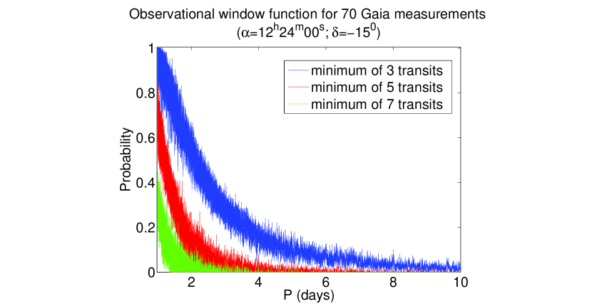
Figure 1: A sample observational window function for a sky direction that Gaia is expected to observe $70$ times, the average expected number of measurements over the entire mission. The detection probability is calculated for transit duration of $2$ hours, for a minimum of three, five and seven observations in transit.

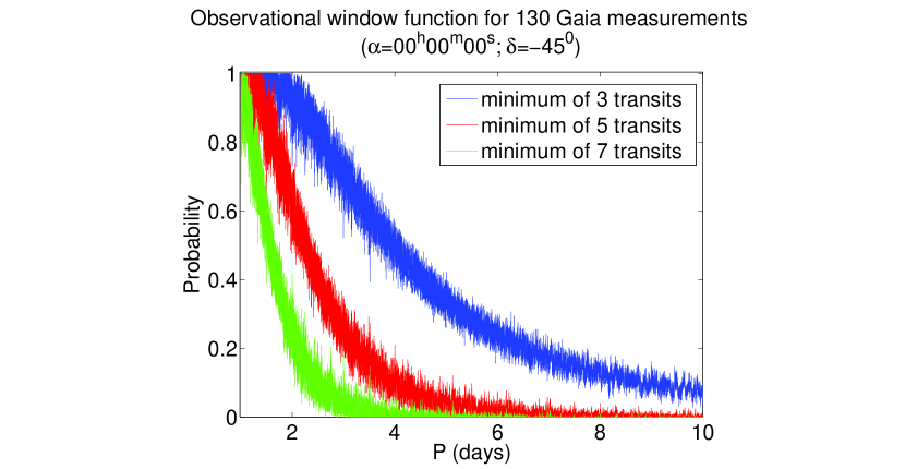
Figure 2: A sample observational window function for an area that Gaia is expected to observe $130$ times.

Since we neglected the dependence of the window function on the SNR and therefore on the stellar characteristics, it remains mainly a function of the period and the scanning law. We can therefore take it out of the integral sign in Eq. 1, which we calculate separately for each patch. We also divided the apparent magnitude range ($G=6-16$) into $1$-mag bins and treated each bin separately. Only at the end of the integration we multiplied the result with the detection probability we obtained from the window function.

3 Results

Table 1 presents the resulting expected yield of transiting HJs and VHJs in Gaia photometry, down to stellar magnitudes $14$ and $16$, for which we expect Gaia to observe on the order of $1.5\times 10^{5}$ and $6.8\times 10^{5}$ stars, respectively. Obviously, the required minimum number of observations in transit strongly affects the results, as well as the assumed transit duration. In Fig. 3 we present the transiting planets yield for a minimum of five sampled transits, for transit duration of $2$ hours, divided into apparent magnitude bins, from $M=6$ to $M=16$. Our results show that the Gaia photometry is expected to yield on the order of hundreds or thousands of new planets, depending on the detection strategy.

Table 1: Gaia expected detections down to a limiting magnitude

	Minimum Number of
	Points in Transit	$G=14$	$G=16$
	3	230	999
$w=1\,\mathrm{hr}$	5	42	178
	7	7	30
	3	596	2605
$w=2\,\mathrm{hr}$	5	209	902
	7	73	310
	3	720	3191
$w=3\,\mathrm{hr}$	5	364	1577
	7	156	669

Note. — The expected yield of HJs and VHJs from Gaia photometry, for three different transit durations, down to a limiting apparent magnitudes of $G=14$, and $G=16$.

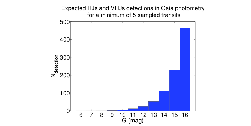
Figure 3: The expected yield broken into apparent magnitude bins. This yield was calculated for a minimum of five sampled transits, and a transit duration of $2$ hours.

Given the large amount of stars that Gaia will measure, we must estimate the false-alarm rate. The probability that $1\,\mathrm{mmag}$ purely white noise will produce a single ’transit-like’ outlier (with magnitude of $0.005-0.015$ mag) is $\sim 3.5\times 10^{-7}$, which amounts to $\sim 2\times 10^{-15}$ for three outliers out of the average $70$ measurements. This is a worst case estimate, as requiring the outliers to have a periodic pattern, even reduces this probability. Thus, under our nominal assumptions, it is obvious that the false-alarm rate is negligible.

Nevertheless, the analysis might be complicated by stellar red noise. If the red noise doesn’t possess a periodic or quasi-periodic nature, then the low-cadence sampling simply renders it “white”, effectively reducing the SNR. According to McQuillan et al. (2012) we estimate that roughly half of the stars have microvariability larger than 2 mmag. This results in an increased false alarm rate. However, in our upcoming paper (Dzigan & Zucker, in preparation) we show that our prioritization process in the Directed Follow-Up approach effectiviely eliminates them.

In any case, Gaia will provide the astrometric and spectroscopic data needed for further classification. These data will help to exclude false-positives, such as background eclipsing binaries (BGEB), and to distinguish between periodic variability of stellar source and planetary transits. Thus, we can conclude that we don’t foresee a significant false-positive rate, as long as we focus our analysis on HJs.

Our results seem to differ considerably from those of Robichon (2002). We suspect that the main cause for the discrepancy is the different scanning law we used, which implied $50-200$ observations per star, with a mean of $70$, compared to $100-300$ with a mean of $130$, which Robichon used. This reflects changes in the mission design during the years that elapsed since 2002. Fig. 1 and Fig. 2 hint at the significant effect this change had on the observational window function.

It is important to stress again that the analysis we present did not consider smaller planets. Their detection will be more difficult, and moreover, the required follow-up, either photometric or spectroscopic, will be more complicated. This topic will require a much more elaborate and careful analysis.

The analysis we present in this Letter is a rough estimate that is based on general assumptions. We obviously made some approximations on the way, but at the level of accuracy needed at this stage we feel they are justified. The most important conclusion is that it will be worth while to develop detection algorithms, that will be tailored for Gaia photometry, and that will be incorporated into the pipeline. This may reduce the minimiun number of points in transit required for detection, which will immensely affect the yield. In addition, establishing a follow-up network that will be able to respond to alerts will also have a crucial effect, again, through this reduction in the number of required observations in transit (e.g. Wyrzykowski & Hodgkin 2011).

A significant feature one can notice while examining Table 1 and Fig. 3 is the very strong dependence of the yield on the limiting apparent magnitude. Extending the analysis to fainter magnitudes will require introduction of the SNR into the analysis. This effort will be useless unless high-precision radial velocities of such faint targets will be feasible. Extremely large telescopes such as the E-ELT may allow this kind of observations. The enormous increase in the number of detected planets with Gaia, if fainter stars are considered, may serve as a justification to build high-precision radial velocity spectrographs for those telescopes.

Gaia will undoubtedly revolutionize astronomy in many aspects. Nevertheless, its contribution to the field of transiting exoplanets is usually expected to be marginal. The expected transiting planet yield is the key factor to establish whether this field will benefit considerably from Gaia. Usually, transit surveys focus on dense fields, to maximize the chances to detect transits and effectively use their high cadence. Gaia, on the other hand, will be an all-sky, low-cadence survey. This kind of surveys are usually considered irrelevant for transit searches. The estimate we present here shows that Gaia will have a valuable and significant contribution also in this field, mainly due to its high photometric precision, and in spite of its low cadence.

4 acknowledgments

This research was supported by The Israel Science Foundation and The Adler Foundation for Space Research (grant No. 119/07). We are grateful to Leanne Guy and Laurent Eyer for fruitful discussions and for providing us with the most updated scanning law of Gaia. We wish to thank the referee Douglas Caldwell whose valuable comments helped to improve this paper.

References

- Bahcall & Soneira (1980) Bahcall J. N., Soneira R. M., 1980, ApJS, 44, 73
- Beatty & Gaudi (2008) Beatty T. G., Gaudi B. S., 2008, ApJ, 686, 1302 (BG)
- de Bruijne (2012) de Bruijne, J. H. J., 2012, Ap&SS, in press (arXiv:1201.3238)
- Dzigan & Zucker (2011) Dzigan, Y., Zucker, S., 2011, MNRAS, 415, 2513
- Gould et al. (2006) Gould, A., Dorsher S., Gaudi B. S., & Udalski A., 2006, Acta Astron., 56, 1
- Haywood et al. (1997) Haywood, M., Robin, A. C., & Creze M., 1997, A&A, 320, 440
- Høg (2002) Høg, E., 2002, Ap&SS, 280, 139
- Howard et al. (2011) Howard, A. W., Marcy, G. W., Bryson, S. T., et al. 2011, arXiv:1103.2541
- Jordi et al. (2010) Jordi, C., Gebran, M., Carrasco, J. M., et al., 2010 A&A, 523, A48
- Kovács et al. (2002) Kovács, G., Zucker, S., & Mazeh, T., 2002, A&A, 391, 369
- Lindegren (2010) Lindegren, L., 2010, in Relativity in Fundamental Astronomy: Dynamics, Reference Frames, and Data Analysis (IAU Symp. 261) IAU Symposium, ed. S. A. Klioner, P. K. Seidelmann, & M. H. Soffel, (Cambridge: Cambridge Univ. Press), 296
- McQuillan et al. (2012) McQuillan, A., Aigrain, S., & Roberts, S. 2012, A&A, 539, A137
- Reid et al. (2002) Reid, I. N., Gizis, J. E., & Hawley S. L., 2002, AJ, 124, 2721
- Robichon (2002) Robichon, N., 2002, EAS Publ. Ser., 23, 19
- Tingley (2011) Tingley, B., 2011, A&AS, 529, A6
- von Braun et al. (2009) von Braun, K., Kane, S. R., & Ciardi, D. R., 2009, ApJ, 702, 779
- Wyrzykowski & Hodgkin (2011) Wyrzykowski L., Hodgkin S., 2011, ArXiv:1112.0187