Resonant enhancement of a single attosecond pulse in a gas medium by a time-delayed control field

Abstract

An optical coherent control scheme has been proposed and theoretically investigated where an extreme ultraviolet single attosecond pulse (SAP) propagates through a dense helium gas dressed by a time-delayed femtosecond laser pulse. The laser pulse couples the $2s2p(^{1}P)$ and $2s^{2}(^{1}S)$ autoionizing states when the SAP excites the $2s2p$ state. After going through the gas, the spectral and temporal profiles of the SAP are strongly distorted. A narrowed but enhanced spike in the spectrum shows up for specific intensities and time delays of the laser, which exemplifies the control of a broadband photon wave packet by an ultrashort dressing field for the first time. We analyze the photon and electron dynamics and determine the dressing condition that maximizes this enhancement. The result demonstrates new possibilities of attosecond optical control.

Single attosecond pulses (SAPs) were produced in the laboratory for the first time in 2001 hentschel . The synchronized pair of an SAP and an infrared (IR) pulse in the so called “pump-probe” scheme has become an indispensable tool over the past decade to time-resolve the electron motion in quantum processes such as photoionization kitzler , Auger emission drescher , tunneling uiberacker , molecular dissociation kelkensberg , and autoionization gilbertson . In most of these experiments, to retrieve the dynamics, the SAP photoionizes the atoms or molecules, and the “probe” IR pulse “streaks” the photoelectrons with different time delays between the pulses. The streaking model is based on electron emission to a structureless continuum energy band. In reality, there are abundant excited states in atoms and molecules, which can be strongly coupled by the IR field. This coupling scheme is not different from that in the electromagnetically induced transparency (EIT) effect marangos ; fleischhauer-rmp , which has been studied extensively since first discovered in the 1990’s harris ; boller using two laser pulses. In fact, the EIT effect has been studied recently in extreme ultraviolet (XUV) loh ; gaarde ; tarana ; pfeiffer and X-ray buth ; glover energies in tens to hundreds of femtoseconds.

Using light to control quantum systems has long been of great interest not only for the fundamental understanding of light-matter interactions, but also for applications in quantum information lukin-rmp , light source generation sansone , ultracold atoms wieman , and precision spectroscopy hall ; hansch . The EIT effect has been a powerhouse for optical coherent control where photoabsorption of light in matter in certain energy range can be reduced by a precisely configured dressing laser. As a prominent application in quantum information, photon storage is achieved by EIT where the refraction index is tuned to transfer information between photonic and atomic states fleischhauer ; liu ; phillips . To achieve efficient coherent transitions, this type of optical control is carried out in nanosecond to microsecond timescales and under perfect resonance condition between long-living quantum states.

Very lately, after the color-shifting of a light pulse was proposed notomi and realized preble using crystals, an alternative approach using the EIT technique with time-delayed pulses was reported ignesti10 . The same approach is also capable of tuning the bandwidth of a propagating light ignesti11 . In the time domain, a transient “transmission gain” has been observed in nanoseconds when the strong dressing field is rapidly switched on or off chen ; echaniz ; greentree . All of these efforts not only elucidate the EIT mechanism, but also promote the level of manipulation of light from the traditional EIT effect to higher degrees of control. However, these techniques are established for narrowband lasers and unable to treat the dynamics initiated by a broadband SAP in attosecond timescales.

The present theoretical work aims to control an SAP going through a laser-dressed gaseous medium by utilizing the state-of-the-art ultrafast technology. We simulate the propagation of an 1-fs XUV pulse (bandwidth 1.8 eV) in a helium gas where the $2s2p(^{1}P)$ and $2s^{2}(^{1}S)$ autoionizing states (AISs) are strongly coupled by a 9-fs laser pulse. The dynamics of the coupled system is controlled by three comparable timescales, given by the autoionization, the population transfer between the two AISs, and the durations of the two light pulses. By tuning the laser intensity and the time delay between the pulses to specific values, a sharp peak, with a 50% increase from the incident signal, shows up in the XUV transmission spectrum at the $2s2p$ resonance. Compared to the transparency window in EIT, it is effectively a photon emission window controlled by the ultrashort dressing laser. The enhanced peak is very localized in energy ($<100$ meV) and in the time delay ($<3$ fs), demonstrating a high-level control of a photon wave packet.

Consider a three-level atom, where the top two levels $|a\rangle$ and $|b\rangle$ are AISs, associated with the background continuum $|E_{1}\rangle$ and $|E_{2}\rangle$, respectively. An XUV (labeled by $X$) pulse couples the ground state $|g\rangle$ to the $|a\rangle$-$|E_{1}\rangle$ resonance, and a laser (labeled by $L$) pulse couples the two resonances, where the radiation fields are treated classically fontana . The coupling scheme can be either ladder- or $\Lambda$-type. For the near-resonance coupling with weak to moderately strong field intensities, the total wavefunction is described by lambropoulos ; bachau ; madsen ; themelis

$$|\Psi(t)\rangle =e^{-iE_{g}t}c_{g}(t)|g\rangle$$ (1)

$$+e^{-iE_{X}t}\left[c_{a}(t)|a\rangle+\int{c_{E_{1}}(t)|E_{1}\rangle dE_{1}}\right]$$

$$+e^{-iE_{L}t}\left[c_{b}(t)|b\rangle+\int{c_{E_{2}}(t)|E_{2}\rangle dE_{2}}\right],$$

where $E_{X}\equiv E_{g}+\omega_{X}$, $E_{L}\equiv E_{g}+\omega_{X}+\omega_{L}$, and the $c(t)$’s are smoothly varying coefficients. The three-level system is schematically plotted in 1. For a given set of atomic levels and external fields, the total wavefunction $|\Psi(t)\rangle$ is uniquely calculated chu11 .

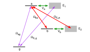
Figure 1: (Color online) Schematic diagram of a three-level atom in two light fields. The arrows represent coupling between the states, labeled by the transition amplitudes. The green arrows are autoionizations, the thin purple arrows are XUV couplings, and the thick red arrows are laser couplings. Only first-order transitions are considered.

By convention, we assume the form of light pulses as $E(t)=F(t)e^{i\omega t}+c.c.$. The envelope $F(t)$ is complex in general, and it is initially a sine-square type real function. All the fast oscillating terms are factored out in the numerical calculation. The dipole moment of the atom is chu12

$$\mu(t)=u_{X}(t)e^{i\omega_{X}t}+u_{L}(t)e^{i\omega_{L}t}+c.c.,$$ (2)

where

$$u_{X}(t) \equiv\left(D_{ag}+i\pi V_{a}D_{E_{1}g}\right)c_{a}^{*}(t)c_{g}(t)$$ (3)

$$-i\pi F_{X}(t)\left|D_{E_{1}g}c_{g}(t)\right|^{2},$$

and $u_{L}(t)$ corresponds to laser frequency, which is not in our concern. The matrix elements $D_{ij}\equiv\langle i|D|j\rangle$ and $V_{a}\equiv\langle E_{1}|H|a\rangle$ are real values by employing standing waves for the continuum basis $|E_{1}\rangle$ and $|E_{2}\rangle$.

For a given set of XUV and laser pulses, the wavefunction $|\Psi(t)\rangle$ and the dipole response $\mu(t)$ are adequate to describe the electron emission and photoabsorption in a dilute gas chu11 ; chu12 . However, in a dense gas, the fields are altered by the response of the atomic medium. By pairing a weak XUV and a moderately strong laser that are different by two orders of magnitude in the intensity, we assume that the laser propagates without modification in the medium. The ionization is weak so the plasma effect is disregarded. The spontaneous decay is much slower than the AIS decay and dismissed in the model.

By redefining the time coordinate in the moving frame $t^{\prime}=t-z/c$ where $z$ is along the traveling direction of the light, the Maxwell equation is written as

$$\frac{\partial E(z,t^{\prime})}{\partial z}=-\frac{\rho}{c\epsilon_{0}}\frac{\partial\mu(z,t^{\prime})}{\partial t^{\prime}},$$ (4)

where $\rho$ is the density of the gas. The dependence in the transverse direction has been removed for loosely focused lights. Factoring out the carrier oscillation terms, the propagation of the XUV field is described by

$$\frac{\partial F_{X}(z,t^{\prime})}{\partial z}=-\frac{\rho}{c\epsilon_{0}}\left[\frac{\partial u_{X}(z,t^{\prime})}{\partial t^{\prime}}+i\omega_{X}u_{X}(z,t^{\prime})\right].$$ (5)

Putting together (3) and (5), one can integrate iteratively to obtain the dipole envelope $u_{X}(z,t^{\prime})$ and the XUV envelope $F_{X}(z,t^{\prime})$ as functions of $t^{\prime}$ at each spatial point $z$ until the pulse exits the medium, which is then defined as the transmitted XUV pulse.

The medium in concern is a 2-mm thick gas of noninteracting helium atoms. The pressure and the temperature are 25 torr and 300 K respectively (density $\rho=8\times 10^{17}$ cm^-3). An XUV pulse (SAP) and a time-delayed laser pulse are colinearly propagated and linearly polarized in the same direction. The 1.8-eV bandwidth of the XUV pulse (central frequency $\omega_{X}=60.15$ eV, duration in full width at half maximum $\tau_{X}=1$ fs, and peak intensity $I_{X}=10^{10}$ W/cm²) is much broader than the 37-meV $2s2p$ resonance. The laser pulse ($\lambda_{L}=540$ nm, $\tau_{L}=9$ fs) resonantly couples $2s2p$ and $2s^{2}$. For convenience, the peak laser intensities ($I_{L}$) are expressed in terms of $I_{0}\equiv 10^{12}$ W/cm². The time delay $t_{0}$ is defined as the time between the two pulse peaks, and it is positive when the XUV peak comes first.

To reproduce the EIT condition as a reference, we apply a 1-ps laser pulse which overlaps temporally with the SAP and calculate the XUV spectra. As seen in 2(a), without the laser, the spectrum simply displays the $2s2p$ Fano lineshape fano . When the laser intensity increases, the Fano peak splits into two with increasing separations. Note that these intensities correspond to linearly increasing field strengths. The split peaks are the exact reproduction of the Autler-Townes doublet autler , where the peak separation is equal to the Rabi frequency. Although our “probe” in this EIT-like setup is, unconventionally, an SAP, as long as the laser is long in terms of the coupling strength, the dressed-state interpretation is valid, and the Autler-Townes phenomenon is recovered. Note that the split lineshapes are broadened due to the 120-meV resonance width of $2s^{2}$.

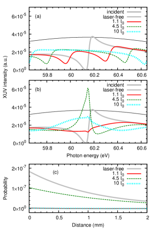
Figure 2: (Color online) (a) XUV spectra near the $2s2p$ resonance with a 1-ps overlapping ($t_{0}=0$) laser. (b) Same as (a) but the laser duration is 9 fs. Various peak laser intensities are applied. (c) The $2s2p$ bound state population at the end of the laser pulse versus the distance inside the gas.

Next, we shorten the laser duration to $\tau_{L}=9$ fs and keep the overlapping condition ($t_{0}=0$). The XUV spectra are plotted in 2(b). For $I_{L}=1.1I_{0}$, the Fano lineshape that appears in the laser-free case is washed out, and the spectrum is almost flat, which indicates that the ionization path through the “bound” $2s2p$ vanishes. For $I_{L}=4.5I_{0}$, the central region of the spectrum turns to an upside-down mirror image of the original Fano lineshape, implying that the path through $2s2p$ has gone through a phase shift of $\pi$, or equivalently, the Fano $q$-parameter changes sign after one Rabi cycle. What is more surprising is that in 60.0-60.2 eV, the transmission signal is actually higher than the incident signal, i.e., the XUV emission is produced at the resonance by the particular coupling condition. However, by further increasing the intensity to $I_{L}=10I_{0}$, the emission signal drops down, and the enhancement feature disappears.

The disappearance of the $2s2p$ peak in the XUV spectrum for certain laser intensities is clarified by the $2s2p$ bound state population $|c_{a}(t)|^{2}$. Its value at the moment the laser pulse ends (12.4 fs) is plotted in 2(c) along the propagation in $z$, before it further decays toward the end of autoionization. Under the laser-free condition, the SAP intensity drops exponentially as it is absorbed along $z$, and thus the excitation of $2s2p$ decreases accordingly. For $I_{L}=1.1I_{0}$, $4.5I_{0}$, and $10I_{0}$, the Rabi oscillation after the SAP runs for 0.5, 1, and 1.5 cycles, respectively, where the $2s2p$ population is either dried up (half-integer cycles) or highly populated (integer cycles). For $I_{L}=4.5I_{0}$, the $2s2p$ residue keeps decaying to the resonance peak, while for $I_{L}=1.1I_{0}$ and $10I_{0}$, the spectra turn to be quite flat.

The comparison in 2(b) shows that the resonant absorption turns to emission only for a specific laser intensity. To investigate the trend further, 3 plots the XUV signal in a 50-meV energy window centered at $2s2p$ (60.15 eV) against the time delay. This spectral resolution is easily reachable in typical spectrometers. Without the laser, the incident and transmitted signals are $7\times 10^{-8}$ and $1\times 10^{-8}$ respectively, i.e., 85% of the light in this window is absorbed by the medium. With the presence of the coupling laser, the signal yield builds up with time delay, reaching a maximum, and then decreases again. As the intensity increases to $I_{L}=4.5I_{0}$, the buildup starts faster, and the maximum yield at $t_{0}=0$ is about 40% higher than the incident signal. For $I_{L}=10I_{0}$, the maximum enhancement increases to about 50% and shifts to $t_{0}=-2$ fs. These extraordinary oscillatory features for different laser intensities could be revealed in an actual XUV-plus-IR type measurement.

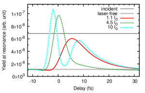
Figure 3: (Color online) Total XUV yields covering a 50-meV window centered at the $2s2p$ resonance against the time delay, for different laser intensities.

To fully understand the mechanism behind this signal oscillation, the dynamics in the time domain is analyzed. Under laser-free condition, the SAP prompts the $2s2p$ state and generates dipole oscillation, which then radiates XUV before the $2s2p$ decays. The transmitted light consists of the leading SAP (“head”) and the longer trailing part (“tail”) due to the emission from the decaying $2s2p$. Their coherent sum results in the original Fano line shape seen in 2. The head and the tail partially cancel each other in the temporally overlapping region due to the phase shift of the dipole radiation, which is analogous to the study carried out for a rectangular pulse propagating in a two-level atomic system shakhmuratov as a form of transient nutation hocker . In the presence of laser coupling, the Rabi oscillation brings the electrons back and forth between the two AISs after the SAP. Every Rabi cycle that brings the electrons back to $2s2p$ adds a phase shift of $\pi$ to the tail. Transmission enhancement occurs when there is just one Rabi cycle to flip the dip part (the minimum) to a maximum due to the additional $\pi$ phase added to the interference. Note that regardless of the laser intensity, the magnitude of the dipole oscillation initiated by the SAP always declines with time. In other words, the earlier the Rabi cycle is accomplished, the stronger the enhancement appears. This aspect is seen by the peak positions and heights of all three curves in 3. This prediction complements the earlier experiment using an attosecond pulse train to enhance the high harmonic signals gademann , which was based on the scheme first conducted to study wave packet interference johnsson . They were related to our study but in a different nature.

As expressed by the propagation in (5), the XUV pulse is shaped by the electric dipole modulated by the 2.3-eV laser field. The process is a form of spectral redistribution of the XUV pulse caused by the oscillation between the AISs. To illustrate the conservation of the total XUV signal in this process, we integrate each curve in 2(b) over an 1-eV range centered at the resonance which covers the essential reshaping region of interest. Without the laser, nearly 40% of the XUV photons are absorbed as the pulse goes through the medium. When the laser is turned on, for all three intensities, the yield decreases only slightly from the laser-free case, by at most about 17%. This extra loss is dissipated via the autoionization of $2s^{2}$, mediated by the coupling laser.

Light traveling in a linear medium attenuates with a constant absorption rate proportional to the medium density, as stated by Beer’s law ishimaru . However, in a strongly coupled medium, this law does not hold anymore, especially for high densities. The XUV transmission spectra for $I_{L}=4.5I_{0}$, $t_{0}=0$, and gas pressures $P=25$, 50, and 75 torr are displayed in 4. The figure shows that the background continuum part is weakened as the pressure rises, but the enhanced peak, while distorted and shifted, remarkably maintains the same height. For $P=75$ torr, the highest transmitted light signal is about 20 times larger than the lowest part in the background. The stability of the enhancement peak is due to the balance between two processes: the light is dragged from the pulse head backward in time ($t^{\prime}$) to the tail, while the tail keeps being absorbed; both processes are accelerated by higher gas densities.

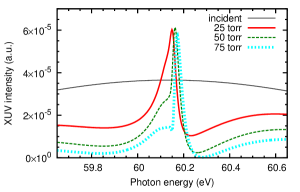
Figure 4: (Color online) Transmitted XUV spectra for the gas pressures of 25, 50, and 75 torr. The laser condition is $\lambda_{L}=540$ nm, $\tau_{L}=9$ fs, $I_{L}=4.5$ TW/cm², and $t_{0}=0$.

In conclusion, we have simulated an 1-fs XUV pulse propagating through a dense gas of three-level autoionizing helium atoms coupled by a time-delayed 9-fs laser. By adjusting the coupling laser to preferred conditions, an enhancement appears at the resonance energy in the XUV transmission spectrum, demonstrating up to a drastic 50% increase in the signal count. The transmitted XUV pulse is composed by the attosecond head part and the longer tail part in the time domain, where the phase of the tail can be sectionally shifted by the laser, forming special interference patterns in the frequency domain. This remarkable feature relies on the cutting edge of ultrafast technologies–both the XUV and laser pulses are considerably shorter than the 17-fs decay lifetime of $2s2p$–to clearly define the timing of the wave packet dynamics. We find that while higher density obstructs the light surrounding the resonance, the enhancement peak can sustain, so that it spikes up more apparently. Our simulation undertakes reasonable experimental setup and conditions. The unique measurable features and the underlying dynamics could invoke the profound possibilities in the attosecond nonlinear optics.

- (1) M. Hentschel, R. Kienberger, Ch. Spielmann, G. A. Reider, N. Milosevic, T. Brabec, P. Corkum, U. Heinzmann, M. Drescher, and F. Krausz, Nature 414, 509 (2001).
- (2) M. Kitzler, N. Milosevic, A. Scrinzi, F. Krausz, and T. Brabec, Phys. Rev. Lett. 88, 173904 (2002).
- (3) M. Drescher, M. Hentschel, R. Kienberger, M. Uiberacker, V. Yakovlev, A. Scrinzi, Th. Westerwalbesloh, U. Kleineberg, U. Heinzmann, and F. Krausz, Nature 419, 803 (2002).
- (4) M. Uiberacker et. al., Nature 446, 627 (2007).
- (5) F. Kelkensberg et. al., Phys. Rev. Lett. 103, 123005 (2009).
- (6) S. Gilbertson, M. Chini, X. Feng, S. Khan, Y. Wu, and Z. Chang, Phys. Rev. Lett. 105, 263003 (2010).
- (7) J. P. Marangos, J. Mod. Opt. 45, 471 (1998).
- (8) M. Fleischhauer, A. Imamoğlu, and J. P. Marangos, Rev. Mod. Phys. 77, 633 (2005).
- (9) S. E. Harris, J. E. Field, and A. Imamoğlu, Phys. Rev. Lett. 64, 1107 (1990).
- (10) K.-J. Boller, A. Imamoğlu, and S. E. Harris, Phys. Rev. Lett. 66, 2593 (1991).
- (11) Z. H. Loh, C. H. Greene, and S. R. Leone, Chem. Phys. 350, 7 (2008).
- (12) M. B. Gaarde, C. Buth, J. L. Tate, and K. J. Schafer, Phys. Rev. A 83, 013419 (2011).
- (13) M. Tarana and C. H. Greene, Phys. Rev. A 85, 013411 (2012).
- (14) A. N. Pfeiffer and S. R. Leone, Phys. Rev. A 85, 053422 (2012).
- (15) C. Buth, R. Santra, and L. Young, Phys. Rev. Lett. 98, 253001 (2007).
- (16) T. E. Glover et. al., Nature Phys. 6, 69 (2010).
- (17) M. D. Lukin, Rev. Mod. Phys. 75, 457 (2003).
- (18) G. Sansone, L. Poletto, and M. Nisoli, Nature Photon. 5, 655 (2011).
- (19) C. E. Wieman, D. E. Pritchard, and D. J. Wineland, Rev. Mod. Phys. 71, S253 (1999).
- (20) J. L. Hall, Rev. Mod. Phys. 78, 1279 (2006).
- (21) T. W. Hänsch, Rev. Mod. Phys. 78, 1297 (2006).
- (22) M. Fleischhauer and M. D. Lukin, Phys. Rev. Lett. 84, 5094 (2000).
- (23) C. Liu, Z. Dutton, C. H. Behroozi, and L. V. Hau, Nature 409, 490 (2001).
- (24) D. F. Phillips, A. Fleischhauer, A. Mair, R. L. Walsworth, and M. D. Lukin, Phys. Rev. Lett. 86, 783 (2001).
- (25) M. Notomi and S. Mitsugi, Phys. Rev. A 73, 051803(R) (2006).
- (26) S. F. Preble, Q. Xu, and M. Lipson, Nature Photon. 1, 293 (2007).
- (27) E. Ignesti, R. Buffa, L. Fini, E. Sali, M. V. Tognetti, and S. Cavalieri, Phys. Rev. A 81, 023405 (2010).
- (28) E. Ignesti, R. Buffa, L. Fini, E. Sali, M. V. Tognetti, and S. Cavalieri, Phys. Rev. A 83, 053411 (2011).
- (29) H. X. Chen, A. V. Durrant, J. P. Marangos, and J. A. Vaccaro, Phys. Rev. A 58, 1545 (1998).
- (30) S. R. de Echaniz, A. D. Greentree, A. V. Durrant, D. M. Segal, J. P. Marangos, and J. A. Vaccaro, Phys. Rev. A 64, 055801 (2001).
- (31) A. D. Greentree, T. B. Smith, S. R. de Echaniz, A. V. Durrant, J. P. Marangos, D. M. Segal, and J. A. Vaccaro, Phys. Rev. A 65, 053802 (2002).
- (32) P. R. Fontana, Atomic radiative processes (Academic Press, New York, 1982), Chap. 5.
- (33) P. Lambropoulos and P. Zoller, Phys. Rev. A 24, 379 (1981).
- (34) H. Bachau, P. Lambropoulos, and R. Shakeshaft, Phy. Rev. A 34, 4785 (1986).
- (35) L. B. Madsen, P. Schlagheck, and P. Lambropoulos, Phys. Rev. Lett. 85, 42 (2000).
- (36) S. I. Themelis, P. Lambropoulos, and M. Meyer, J. Phys. B: At. Mol. Opt. Phys. 37, 4281 (2004).
- (37) W.-C. Chu, S.-F. Zhao, and C. D. Lin, Phys. Rev. A 84, 033426 (2011).
- (38) W.-C. Chu and C. D. Lin, Phys. Rev. A 85, 013409 (2012).
- (39) U. Fano, Phys. Rev. 124, 1866 (1961).
- (40) S. H. Autler and C. H. Townes, Phys. Rev. 100, 703 (1955).
- (41) R. N. Shakhmuratov, Phys. Rev. A 85, 023827 (2012).
- (42) G. B. Hocker and C. L. Tang, Phys. Rev. Lett. 21, 591 (1968).
- (43) G. Gademann, F. Kelkensberg, W. K. Siu, P. Johnsson, M. B. Gaarde, K. J. Schafer, and M. J. J. Vrakking, New J. Phys. 13, 033002 (2011).
- (44) P. Johnsson, J. Mauritsson, T. Remetter, A. L’Huillier, and K. J. Schafer, Phys. Rev. Lett. 99, 233001 (2007).
- (45) A. Ishimaru, Wave propagation and scattering in random media (IEEE Press, New York, 1997), Chap. 6.