Laser-assisted-autoionization dynamics of helium resonances
with single attosecond pulses

Abstract

The strong coupling between two autoionizing states in helium is studied theoretically with the pump-probe scheme. An isolated 100-attosecond XUV pulse is used to excite helium near the $2s2p(^{1}P)$ resonance state in the presence of an intense infrared (IR) laser. The laser field introduces strong coupling between $2s2p(^{1}P)$ and $2p^{2}(^{1}S)$ states. The IR also can ionize helium from both autoionizing states. By changing the time delay between the XUV and the IR pulses, we investigated the photoelectron spectra near the two resonances. The results are used to explain the recent experiment by Gilbertson et al [Phys. Rev. Lett. 105, 263003 (2010)]. Using the same isolated attosecond pulse and a 540 nm laser, we also investigate the strong coupling between $2s2p(^{1}P)$ and $2s^{2}(^{1}S)$ by examining how the photoelectron spectra are modified vs the time delay and the possibility of observing Autler-Townes doublet in such experiments.

I Introduction

Quantum coherence is essential to the understanding and control of the dynamics in a quantum system. With the advances of experimental techniques and technologies, extreme ultraviolet (XUV) attosecond pulse trains (APT) and single attosecond pulses (SAP) have been produced through the high-order harmonic generation (HHG) process, by exposing atoms to intense infrared lasers. Since the natural time scale of the electronic motion of valence electrons in atoms and molecules is in the order of hundreds of attoseconds, these pulses can be used to manipulate or control electron dynamics at the attosecond level krausz . For this purpose, pump-probe scheme is used experimentally where the dynamics of the system is investigated by varying the time delay between the pulses. However, existing XUV SAP and APT are too feeble to be used for XUV-pump-XUV-probe measurements. Instead, most of the experiments have been carried out using the weak XUV-pump with an intense IR-probe pulse. Rigorously speaking, the IR can be considered as a probe only if it is applied after the XUV pump ends. In such case, the electron wave packet generated by the APT or the SAP is probed. In most experiments, however, measurements are also made where the XUV and IR overlap in time. Since the IR is much stronger than the XUV, such measurements are better understood as laser-assisted photoionization.

In XUV+IR experiments, the interaction of the XUV+IR field with the target atom is a nonlinear process. To treat such problems theoretically, the brute-force numerical solution of the time-dependent Schrödinger equation (TDSE) has been carried out by many groups where the target atom is treated within the single electron approximation. For APT+IR, Floquet approach tong10 has also been employed as well. With much efforts, TDSE calculations have been performed for two-electron helium atom and two-electron hydrogen molecules and compared with measurements kelkensberg-sap ; kelkensberg-apt ; sansone . Still, simplified theoretical models are highly desirable in order to acquire a better understanding of the dynamics. These models, clearly, have to depend on the physical systems on hand. To be specific, we will focus on helium atom where many experiments have been carried out.

The first type of XUV+IR experiments used APT where the photon energy runs from below to above the single ionization threshold of helium johnsson ; ranitovic10 ; ranitovic11 ; mauritsson ; shivaram . Spectra of electrons or ions have been measured and calculations based on TDSE and Floquet theory reported johnsson ; ranitovic11 . In the limit of non-overlapping APT and IR, a simplified theory has been reported where the aim was to extract the electron wave packet generated by the APT choi . Alternatively, photon spectra can also be measured holler . In this case, effect due to propagation in the medium has to be considered gaarde . As the energy of the XUV photon increases beyond the single-ionization threshold, it enters a structureless spectral region (about 25 to 55 eV). In this case, the addition of an intense IR to the XUV is to shift the momentum of the continuum electron along the polarization direction of the IR laser, resulting in the ”streaking” of photoelectrons where the energies depend on the vector potential of the IR laser at the time of the electron emission. A ”streaking” theory based on the strong field approximation (SFA) kitzler has been widely used. This theory also forms the basis of the frequency-resolved optical gating for complete reconstruction of attosecond bursts method mairesse for extracting the pulse duration of an SAP. At a still higher photon energy of 60 eV, the XUV alone will reach the spectral region where doubly-excited states of helium are located. In this paper, we will focus on this energy region and consider the dynamics of the doubly excited state generated by the XUV pulse in the presence of an IR pulse at different delay times.

Doubly excited states have been widely studied using synchrotron radiations since the 1960’s madden ; domke91 . These are autoionizing states where the lifetime of a state is typically of a few to tens of femtoseconds. These lifetimes are deduced from the measured spectral width; thus high-precision spectroscopic measurement is needed. With the emergence of SAP, the lifetime of an Auger resonance was first measured in the time domain and analyzed by the XUV+IR streaking theory in 2002 drescher . However, the evolution of the spectral shape of a resonance state has not been determined so far in the time-domain measurements, which in principle can be investigated with attosecond pulses. In fact, the autoionization theory was formulated in the energy domain by Fano fano . This issue was addressed recently by us chu and an experimental scheme was proposed. The scheme, however, requires an attosecond XUV-pump to create the resonance and an attosecond XUV-probe to project out the time-evolution of the resonance. Such measurement is not possible yet. Thus for the time domain measurements so far, doubly-excited states still have to be ”probed” using an IR pulse. For an isolated Fano resonance generated in a combined XUV+IR pulse, the problem has been examined by Wickenhauser et al wickenhauser . A simpler model was proposed by Zhao et al zhao based on SFA.

An XUV+IR experiment on helium doubly-excited states has been reported by Loh et al loh , where a 30 fs XUV pulse was used to excite the $2s2p(^{1}P)$ doubly excited state in the presence of a 42 fs IR laser. The absorption spectra near the $2s2p$ resonance were measured vs the time delay between the pulses. The result was then interpreted by a theory that includes the strong coupling between the $2s2p$ and $2p^{2}(^{1}S)$ states by the IR. In this experiment, the pulse duration of the XUV was longer than the lifetime of the $2s2p$ autoionizing state, i.e., the bandwidth of the light was narrower than the resonance width. Thus, the continuum electrons in a measurement did not have a meaningful “distribution” for such a narrow bandwidth. A single pump could not reveal any significant spectroscopic features; instead, sequential measurements were made where the detuning of the XUV was controlled and scanned through an energy range. The scanned spectra were able to exhibit the autoionization modified by the time-delayed IR, thus providing the temporal information of the system partially. More recently, an 100 as SAP was used by Gilbertson et al gilbertson to excite helium in the presence of a 9 fs IR pulse. The central energy of the excitation is at the $2s2p$ resonance, and the photoelectron spectra near this resonance vs time delay were reported. The result was interpreted based on the theory of Zhao et al zhao from which the decay lifetime of $2s2p$ was retrieved. However, the spectral shape of the resonance was not analyzed due to the limited resolution of 0.7 eV of the electron spectrometer. In contrast to Ref. loh , the interpretation was made by the streaking model of Zhao et al zhao only. Since the IR wavelength used in the two experiments are about the same, the role of strong coupling between the $2s2p$ and $2p^{2}$ states in this experiment should be addressed. This is the goal of the present paper.

The present analysis limits the Hilbert space to including only the two autoionizing states, $2s2p$ and $2p^{2}$, and the ground state. While the XUV can populate other higher doubly excited states, they are weaker in the spectrum and are easily ionized by the IR. Governed by the detuning of the 9 fs IR, only the $2s2p$ and $2p^{2}$ states are strongly coupled. The dynamics of such a system is then studied with a theory generalized from the standard three-level system formulated earlier lambropoulos ; bachau ; madsen ; themelis . To be specific, we develop a model for the IR-dressed autoionization of the $2s2p$ resonance in helium excited by an SAP, where the IR strongly couples the $2s2p$ and $2p^{2}$ resonances and also ionizes both doubly-excited states. Both effects by the IR have to be included in order to explain the observed electron spectra reported in Ref. gilbertson . After achieving good agreement with the experiment, we further investigate the case where $2s2p$ and $2s^{2}(^{1}S)$ are coupled by changing the laser wavelength to 540 nm. The latter state has a higher binding energy such that it is not ionized by the laser. Such measurements would be closer to the standard electromagnetically induced transparency (EIT) experiment harris ; fleischhauer . We will look for the presence of the Autler-Townes doublet autler which are routinely generated by three-level systems with long pulses.

In Sec. II, the model system is defined and the method is introduced. In Sec. III, we show and analyze the results of the two cases, with laser wavelengths $\lambda_{L}=780$ and 540 nm, respectively. For $\lambda_{L}=780$ nm, our calculation is compared with the available experiment gilbertson and with the streaking model based on the SFA model of Zhao et al zhao . For $\lambda_{L}=540$ nm, the results are analyzed, and the possible experimental realization are discussed. In Sec. IV, we give the conclusion. Atomic units (a.u.) are used in Sec. II. In the rest of the paper, electron Volts (eV) and femtoseconds (fs) are used for energy and time, respectively, unless otherwise specified.

II Theory

II.1 General description of the model system

Consider an atomic system with ground state $|g\rangle$ and two doubly excited states $|a\rangle$ and $|b\rangle$. The dipole transition is allowed between $|g\rangle$ and $|a\rangle$ and between $|a\rangle$ and $|b\rangle$. Suppose their energy levels and the external fields are arranged in a way such that the XUV is near resonance between $|g\rangle$ and $|a\rangle$ and the laser is near resonance between $|a\rangle$ and $|b\rangle$. The total time-dependent wave function of the system can be approximately written as

$$|\Psi(t)\rangle =e^{-iE_{g}t}c_{g}(t)|g\rangle$$

$$+e^{-iE_{X}t}\left[d_{a}(t)|a\rangle+\int{d_{E_{1}}(t)|E_{1}\rangle dE_{1}}\right]$$

$$+e^{-iE_{L}t}\left[d_{b}(t)|b\rangle+\int{d_{E_{2}}(t)|E_{2}\rangle dE_{2}}\right],$$ (1)

where $E_{g}$ is the ground state energy, $E_{X}\equiv E_{g}+\omega_{X}$ and $E_{L}\equiv E_{g}+\omega_{X}+\omega_{L}$ are the “pumped energies” with respect to the photon energies $\omega_{X}$ and $\omega_{L}$, where $X$ is for XUV and $L$ is for laser; $|E_{1}\rangle$ and $|E_{2}\rangle$ are the continua with respect to $|a\rangle$ and to $|b\rangle$. The fast oscillating parts in the wave function have been factored out, and the $c(t)$ and $d(t)$ functions are assumed slowly-varying with time. By convention, we use symbol $c(t)$ for coefficients if the expansion is with respect to eigenstates, and symbol $d(t)$ is used when the expansion is in terms of configurations (not eigenstates). The total Hamiltonian of the atomic system in the external fields is

$$H(t)=H_{A}+H_{X}(t)+H_{L}(t),$$ (2)

where $H_{A}$ is the atomic Hamiltonian, and $H_{X}(t)$ and $H_{L}(t)$ represent the interactions of the XUV and laser fields with the atom, respectively. In the photon energy range in consideration, the interaction with the field is given by the electric dipole transition. Equation 2 provides the total Hamiltonian to solve the time-dependent Schrödinger equation for the wave function in Eq. 1, i.e.,

$$i\frac{d}{dt}|\Psi(t)\rangle=H(t)|\Psi(t)\rangle.$$ (3)

The fields are assumed linearly polarized in the same direction. The electric fields are in the form of

$$E(t) =2F(t)\cos(\omega t)$$

$$=F(t)\left(e^{i\omega t}+e^{-i\omega t}\right),$$ (4)

where $2F(t)$ is the pulse envelope. The present model works for arbitrary pulse envelopes; however, we limit the envelope to cosine-square shape in the calculation, i.e.,

$$F(t)=F_{0}\cos^{2}\left(\frac{t-t_{0}}{\tau}\right)\;\text{for}\;-\frac{\pi\tau}{2}<t-t_{0}<\frac{\pi\tau}{2}$$ (5)

and $F(t)=0$ anywhere else, where $t_{0}$ is the peak time. For such a pulse, the pulse duration is $\pi\tau/2.75$, and $F_{0}$ is related to the peak intensity $I_{0}$ by $I_{0}=4F_{0}^{2}$. In this paper, the pulse duration is defined by the full width at half maximum (FWHM) of the intensity envelope. The time delay between the two pulses is define as the time of laser peak subtracted by the time of XUV peak, so it is positive if the peak of the XUV appears before the IR. By convention, in this paper, the XUV peak and the IR peak are placed at $t=0$ and $t=t_{0}$ respectively, so the time delay is $t_{0}$.

Note that the basis functions for the autoionizing states in Eq. 1 are not the eigenstates of the atomic Hamiltonian $H_{A}$. In the basis space of Eq. 1, the diagonal terms of the Hamiltonian are just the energies $E_{g}$, $E_{a}$, $E_{1}$, $E_{b}$, and $E_{2}$. The off-diagonal terms are

$$\langle E_{1}|H(t)|a\rangle =V_{a}$$ (6)

$$\langle E_{2}|H(t)|b\rangle =V_{b},$$ (7)

$$\langle a|H(t)|g\rangle =-D_{ag}F_{X}(t)e^{-i\omega_{X}t}$$ (8)

$$\langle E_{1}|H(t)|g\rangle =-D_{1g}F_{X}(t)e^{-i\omega_{X}t}$$ (9)

$$\langle b|H(t)|a\rangle =-D_{ba}F_{L}(t)e^{-i\omega_{L}t}$$ (10)

$$\langle E_{2}|H(t)|a\rangle =-D_{2a}F_{L}(t)e^{-i\omega_{L}t}$$ (11)

where the $D$ are the dipole matrix elements and $V$ the transition amplitudes of configuration interaction (CI). These terms are schematically plotted in Fig. 1.

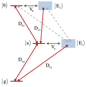
Figure 1: (Color online) Diagram for off-diagonal terms of the Hamiltonian in the configuration basis. The double-arrows represent the transitions between the basis vectors; the red ones represent the dipole transitions, the green ones represent the CIs responsible for autoionization, and the gray dashed ones are neglected in the model.

For the process in concern, additional simplifications are made. Helium atom is taken as a prototype, where $|g\rangle$ is $1s^{2}(^{1}S)$, $|a\rangle$ and $|b\rangle$ are $2s2p(^{1}P)$ and $2p^{2}(^{1}S)$, and $|E_{1}\rangle$ and $|E_{2}\rangle$ are $1s\epsilon p(^{1}P)$ and $1s\epsilon s(^{1}S)$, respectively. Referring to Fig. 1, since the IR coupling is a one-electron dipole operator, the coupling between $2p^{2}(^{1}S)$ and $1s\epsilon p(^{1}P)$ is zero to the first order. The coupling between the two continuum states by the dipole operator can also be neglected since the IR is not absorbed by the continuum electron. We also use the rotating wave approximation such that only the resonant transitions are considered. Furthermore, the matrix elements involving continuum states $|E_{1}\rangle$ and $|E_{2}\rangle$ are assumed energy-independent, which means $D$ and the Fano parameters, $\Gamma$ and $q$, are constant values estimated at the resonances. This is a good approximation when the resonance energy is high enough above the threshold relative to its width so that the continuum only varies slightly across the resonance. In Eqs. 6-11, the basis functions are real by convention (the continua are standing waves) so that all the $D$ and $V$ are real. In this model, all the atomic parameters ($D$, $E$, $\Gamma$, and $q$) are taken from experiments or from calculations in the literature. These parameters are determined by the atomic structure which is irrelevant to the development of our model.

II.2 Three-state model

Under the approximations outlined above, a system of coupled equations for all the coefficients appearing in Eq. 1 are obtained. Considering the conservation of the total probability of the wave packet, the continuum-state coefficients change with time much more slowly than the bound-state coefficients. Thus, $d_{E_{1}}(t)$ and $d_{E_{2}}(t)$ are adiabatically eliminated by assuming their time-derivatives are zeros madsen ; themelis . This allows us to reduce the calculation to include only the bound states. Solving the coupled equations is then numerically feasible. Now we have

$$i\dot{c}_{g}(t) =-i\frac{\gamma_{g}(t)}{2}c_{g}(t)+\lambda_{a}F_{X}(t)d_{a}(t)$$ (12)

$$i\dot{d}_{a}(t) =\lambda_{a}F_{X}(t)c_{g}(t)-\left[\delta_{X}+i\frac{\Gamma_{a}+\gamma_{a}(t)}{2}\right]d_{a}(t)$$

$$+\lambda_{b}F_{L}(t)d_{b}(t)$$ (13)

$$i\dot{d}_{b}(t) =\lambda_{b}F_{L}(t)d_{b}(t)-\left(\delta_{X}+\delta_{L}+i\frac{\Gamma_{b}}{2}\right)d_{b}(t),$$ (14)

where $\lambda_{a}\equiv-D_{ag}(1-i/q_{a})$ and $\lambda_{b}\equiv-D_{ba}(1-i/q_{b})$ are the newly defined complex dipole matrix elements which include the route through the continua. The laser-induced broadening $\gamma_{g}(t)$ and $\gamma_{a}(t)$ are defined by

$$\gamma_{g}(t) \equiv 2\pi\left|D_{1g}F_{X}(t)\right|^{2}$$ (15)

$$\gamma_{a}(t) \equiv 2\pi\left|D_{2a}F_{L}(t)\right|^{2},$$ (16)

the detuning of the pulses are $\delta_{X}\equiv\omega_{X}+E_{g}-E_{a}$ and $\delta_{L}\equiv\omega_{L}+E_{a}-E_{b}$, and the Fano parameters are $\Gamma_{a}\equiv 2\pi|V_{a}|^{2}$, $\Gamma_{b}\equiv 2\pi|V_{b}|^{2}$, $q_{a}\equiv D_{ag}/(\pi V_{a}D_{1g})$, and $q_{b}\equiv D_{ba}/(\pi V_{b}D_{2a})$. The AC Stark shifts vanish, i.e.,

$$P\int{\frac{|D_{1g}F_{X}(t)|^{2}}{E_{X}-E_{1}}dE_{1}}=P\int{\frac{|D_{2a}F_{L}(t)|^{2}}{E_{L}-E_{2}}dE_{2}}=0$$ (17)

because $D_{1g}$ and $D_{2a}$ are constant of energy, where $P$ means the principal part.

With any given set of atomic parameters, field parameters, and initial conditions, Eqs. 12-14 uniquely determine the bound-state part of the total wave function regardless of the continua. In numerical calculations, we propagate these coefficients using the Runge-Kutta method, with the initial conditions $c_{g}(t_{i})=1$ and $d_{a}(t_{i})=d_{b}(t_{i})=0$, i.e., the system is in the ground state at initial time $t_{i}$ before the pulses arrive. Note that the model described above retrieves only the bound-state part of the total wave function. It has been applied successfully for long pulses where the photoelectron distribution in each single measurement is disregarded bachau ; madsen ; themelis ; loh . In the present study, however, a broadband XUV pumps the electrons to the continuum and to the bound state alike; missing the continuum coefficients means missing the essential information of the total wave function. In the following, we aim to extend the model to recover the dynamics of the complete system for short-pulse cases.

II.3 Continuum states

The original coupled equations for the continuum states before the adiabatic elimination are

$$i\dot{d}_{E_{1}}(t) =-D_{1g}F_{X}(t)c_{g}(t)+V_{a}d_{a}(t)+(E_{1}-E_{X})d_{E_{1}}(t)$$ (18)

$$i\dot{d}_{E_{2}}(t) =-D_{2a}F_{L}(t)d_{a}(t)+V_{b}d_{b}(t)+(E_{2}-E_{L})d_{E_{2}}(t).$$ (19)

Assuming $\dot{d}_{E_{1}}(t)=\dot{d}_{E_{2}}(t)=0$ in Eqs. 18-19, the approximate $d_{E_{1}}(t)$ and $d_{E_{2}}(t)$ have singularities at $E_{1}=E_{X}$ and at $E_{2}=E_{L}$, respectively. When plugged into the bound-state coupled equations, these singularities are handled properly with contour integrations. After solving Eq. 12-14, the bound-state coefficients $c_{g}(t)$, $d_{a}(t)$, and $d_{b}(t)$ are known functions of time. We then return to the full version of the continua in Eq. 18-19 to retrieve $d_{E_{1}}(t)$ and $d_{E_{2}}(t)$, again by the Runge-Kutta propagation over time, with the initial conditions $d_{E_{1}}(t_{i})=d_{E_{2}}(t_{i})=0$. The new $d_{E_{1}}(t)$ and $d_{E_{2}}(t)$ functions generated by Eq. 18-19 are the next iteration and better solutions to the previous ones.

After the pulses are over, the system may still change due to autoionization. For an arbitrary set of bound- and continuum-state coefficients, the photoelectrons evolve to a final energy distribution after about 10 times the decay lifetime or so chu . To simulate this measurable photoelectron spectrum, we have to project the total wave packet that has propagated for a long time onto the partial waves of interest; equivalently, taking the $|a\rangle$-$|E_{1}\rangle$ resonance for example, the spectrum is proportional to $|d_{E_{1}}(t_{f})|^{2}$ as $t_{f}\to\infty$. The probability density of the continuum wave function, $P(E_{1})\equiv|d_{E_{1}}(t_{f})|^{2}$, is called “photoelectron profile” or simply “profile” hereafter in this paper. Numerically, $t_{f}$ is taken when $|d_{E_{1}}(t)|^{2}$ does not change anymore. In the case concerning the $2s2p(^{1}P)$ resonance in helium, the decay lifetime is 17 fs, so the final spectrum can be safely taken at about $t_{f}=200$ fs. Note that $P(E_{1})$ has the dimension of probability per unit of energy, and the integral of $P(E_{1})$ over energy represents the total probability of the system being in the $|E_{1}\rangle$ continuum. The conservation of total probability can be used to numerically check the convergence of calculation. The continuum states calculated this way have some advantages. First, each of them can be turned on separately once the bound-state calculation is done. Second, the energy range and energy mesh can be arbitrarily chosen without lowering the accuracy because $d_{E_{1}}(t)$ and $d_{E_{2}}(t)$ are calculated independently for each energy point.

In the present work, we only concern ourselves with the final photoelectrons reaching the detector. However, if one wants to know the evolution of electrons in real time before the end of decay, the retrieval of $|d_{E_{1}}(t)|^{2}$ and $|d_{E_{2}}(t)|^{2}$ as functions of energy and time will be the answer, instead of $P(E_{1})$ and $P(E_{2})$ as just functions of energy. The measurement of this short-time behavior was proposed using an additional high-energy short pulse to ionize the inner electron chu .

II.4 Eigenstates

The atomic eigenstates near a resonance are solved in terms of the corresponding bound state and background continuum by Fano’s theory fano . This leads us to express the total wave function in eigenstate basis in the general form of

$$|\Psi(t)\rangle =e^{-iE_{g}t}c_{g}(t)|g\rangle+e^{-iE_{X}t}\int{c_{E}^{(a)}(t)|\psi_{E}^{(a)}\rangle dE}$$

$$+e^{-iE_{L}t}\int{c_{E^{\prime}}^{(b)}(t)|\psi_{E^{\prime}}^{(b)}\rangle dE^{\prime}},$$ (20)

where the superscripts $(a)$ and $(b)$ indicate the $|a\rangle$-$|E_{1}\rangle$ pair and the $|b\rangle$-$|E_{2}\rangle$ pair, respectively. The eigenstates we refer to are the eigenstates of atomic Hamiltonian $H_{A}$, so they are stationary only in the absence of field. In the following, we will discuss only the subspace spanned by $|a\rangle$ and $|E_{1}\rangle$ in details, while the same principles apply to $|b\rangle$ and $|E_{2}\rangle$. In the meantime the superscript $(a)$ is omitted.

The solutions for an eigenstate of energy $E$ in configuration basis is

$$|\psi_{E}\rangle=\mu_{E}|a\rangle+\int{\nu_{EE_{1}}|E_{1}\rangle dE_{1}},$$ (21)

where the coefficients are

$$\mu_{E} =\frac{\sin\theta_{E}}{\pi V_{a}}$$ (22)

$$\nu_{EE_{1}} =\frac{\sin\theta_{E}}{\pi(E-E_{1})}-\cos\theta_{E}\delta(E-E_{1}),$$ (23)

where

$$\theta_{E}\equiv-\tan^{-1}\left(\frac{\Gamma_{a}/2}{E-E_{a}}\right).$$ (24)

The conversion between Eq. 1 and Eq. 20 means that for the $|a\rangle$ resonance,

$$\int{c_{E}(t)|\psi_{E}\rangle dE}=d_{a}(t)|a\rangle+\int{d_{E_{1}}(t)|E_{1}\rangle dE_{1}}.$$ (25)

Starting with Eq. 21 and Eq. 25, with some algebra, the $c_{E}(t)$ coefficients are

$$c_{E}(t)=\frac{\sin\theta_{E}}{\pi V_{a}}d_{a}(t)-(\cos\theta_{E}-i\sin\theta_{E})d_{E_{1}}(t)\big{|}_{E_{1}=E},$$ (26)

which enables us to calculate the detected photoelectron spectrum $P(E)\equiv|c_{E}(t_{f})|^{2}$ as $t_{f}\to\infty$. This spectrum defined here will reach the same result as $P(E_{1})$ defined in Sec. II.3, but just from a different calculation procedure.

The profile $|c_{E}(t)|^{2}$ evolves differently from $|d_{E_{1}}(t)|^{2}$. As pointed out in Sec. II.3, $|d_{E_{1}}(t)|^{2}$ evolves until the end of the decay, and $|c_{E}(t)|^{2}$ evolves until the field is over. In a typical case where the field ends much earlier than the end of the decay, it is more efficient to calculate the final $|c_{E}(t_{f})|^{2}$ than the final $|d_{E_{1}}(t_{f})|^{2}$. Moreover, in Eq. 26, for a point in time and in energy $(t,E)$, the coefficient $c_{E}(t)$ is calculated by a simple algebra with the $d_{a}(t)$ and $d_{E_{1}}(t)|_{E_{1}=E}$ of just the same $(t,E)$; there is no integral over energy nor propagation over time to carry out $c_{E}(t)$ once $d_{a}(t)$ and $d_{E_{1}}(t)|_{E_{1}=E}$ are known. In other words, including $c_{E}(t)$ in the calculation requires very little extra efforts. Summing up these facts, for the purpose of retrieving the electron spectra, it is advantageous to adopt $P(E)=|c_{E}(t_{f})|^{2}$ instead of keeping the form of $P(E_{1})=|d_{E_{1}}(t_{f})|^{2}$. We have come to the conclusion that for the present system and setup, the optimal workflow is in the consecutive order of bound states, continuum states, and eigenstates, all of which calculated in the physical time until the field vanishes.

For the subspace spanned by $|b\rangle$ and $|E_{2}\rangle$, the eigenstate coefficients are constructed by $d_{b}(t)$ and $d_{E_{2}}(t)$ in the same way but with different parameters. Now both $c_{E}^{(a)}(t)$ and $c_{E}^{(b)}(t)$ are obtained, and we can fully build the total wave function in eigenstates basis as shown in Eq. 20.

III Results and discussions

III.1 Laser wavelength of 780 nm

III.1.1 Calculation and analysis

We first apply the model to the case where the laser couples $2s2p(^{1}P)$ and $2p^{2}(^{1}S)$ in helium with the experimental setup reported by Gilbertson et al gilbertson . The two doubly excited states autoionize to $1s\epsilon p(^{1}P)$ and $1s\epsilon s(^{1}S)$ respectively. The measured quantity is the electron spectrum, corresponding to $P(E)=|c_{E}(t_{f})|^{2}$ in the model introduced in Sec. II.4, where $t_{f}$ is taken after the field vanishes. For the XUV pulse, the photon energy is 60 eV and the duration is 100 as; the bandwidth is 20 eV, which is much wider than the width of $2s2p$, and viewed as a flat background in spectrum near the resonance. The XUV transition from the $1s^{2}(^{1}S)$ ground state to $2s2p$ is nearly resonant, and we conveniently set $\delta_{X}=0$. In principle, such pump pulse can initiate other $2snp$, $2pns$ and $2pnd$ states which should all be included in the total wave function. (For more accurate description of doubly excited states, see Lin lin86 ) Nonetheless, those higher states have longer lifetimes, exhibiting less dynamics in the time scale in our scheme; furthermore, their resonance widths are narrow and difficult to measure with typical electron spectrometers. Thus, we treat $2s2p$ as the only $|a\rangle$ state in Eq. 1, while $1s\epsilon p$ is $|E_{1}\rangle$. The Fano parameters of the $2s2p$ resonance are experimental values taken from the literature domke96 , where $E_{a}=60.15$ eV, $\Gamma_{a}=37$ meV, and $q_{a}=-2.75$. The XUV is weak and in the linear regime so that its intensity does not affect the spectra other than an overall factor. The peak XUV intensity is assumed $I_{X}=10^{10}$ W/cm².

The laser pulse is a 9 fs IR pulse with wavelength $\lambda_{L}=780$ nm and peak intensity $I_{L}=7\times 10^{11}$ W/cm². With 1.6 eV photon energy, the IR field couples $2s2p$ and $2p^{2}$ at 62.06 eV, where $\delta_{L}=-0.4$ eV. The atomic parameters $\Gamma_{b}=5.9$ meV burgers and $D_{ba}=2.17$ a.u. loh are taken from literature. The bound-free dipole matrix element $D_{2a}$ responsible for the transition from $2s2p$ to $1s\epsilon s$ is very small because it is a second order (satellite) transition and requires electron correlation, while $D_{ba}$ between $2s2p$ and $2p^{2}$ is a first-order transition via $\langle 2s|D|2p\rangle$. The parameter $q_{b}$, representing the ratio of $D_{ba}$ to $D_{2a}$, is thus very large; it is set $q_{b}=1000$. Note that when $|q|\gg 1$, the Fano shape appears as a symmetric peak, and the sign of $q$ is insignificant.

In order to understand the dynamics controlled by the laser, we evaluate the generalized Rabi frequency defined by

$$\Omega(t)\equiv\sqrt{|D\cdot E(t)|^{2}+|\delta|^{2}}.$$ (27)

When the detuning is large, the Rabi frequency is higher; however, the amplitude of the oscillation is lower, i.e., the population does not fully swing to the other coupled state. In our system and setup, $\Omega=0.43$ eV between $2s2p$ and $2p^{2}$ at the laser peak, corresponding to 9.6 fs period. For the two doubly excited states, the binding energies of $2s2p$ and $2p^{2}$ are 5.3 and 3.3 eV, which are low enough such that their ionizations are quick, especially the latter one. We calculate the ionization rates for both states using the model developed by Perelomov, Popov, and Terent’ev ppt , referred by the PPT model hereafter, with the high-intensity correction introduced in tong05 . The empirical parameters in our PPT calculation are obtained by fitting our result to the experiment, which will be discussed in Sec. III.1.2. The calculated peak rates for $2s2p$ and $2p^{2}$, in units of energies, are 5.4 meV and 0.46 eV, comparable to their resonance widths 37 meV and 5.9 meV, respectively. To incorporate these ionization rates to our coupling model in Eqs. 12-14, the widths are broadened by $\Gamma_{a,b}^{\prime}(t)=\Gamma_{a,b}+W_{a,b}(t)$ where $W_{a}(t)$ and $W_{b}(t)$ are the time-dependent ionization rates for $2s2p$ and $2p^{2}$ respectively. Note that for the dynamics we have considered so far, on one hand, the coupling and the ionization of resonances exist only in the presence of laser field; on the other hand, the autoionization processes are determined exclusively by the atomic structure, whose time scale can not be changed externally.

The probabilities of the $2s2p$ and $2p^{2}$ bound states are presented in Fig. 2 as they propagate in time. Although the bound states are not directly measured in this pump-probe scheme, the analysis therein helps reveal the physics behind the whole time-dependent process. We will analyze the bound-state propagation and the resonance profiles in the following at the same time.

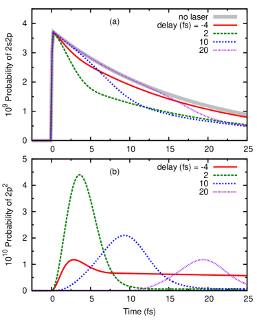
Figure 2: (Color online) Probabilities of the (a) $2s2p$ and (b) $2p^{2}$ bound states with time, for $\lambda_{L}=780$ nm and various $t_{0}$. The case without laser is plotted in the gray solid curve in (a).

The photoelectron profiles of the $2s2p$ resonance for $t_{0}=-10$ to 50 fs are shown in Fig. 3. If the laser field is absent, the dynamics of the system after the pump will be nothing more than the autoionization of $2s2p$, and the detector will see an original Fano line-shape as seen in the absorption spectrum in synchrotron radiation experiment. When a laser is added very early, e.g., $t_{0}=-10$ fs, the spectrum only changes insubstantially because the laser is already gone by the time the XUV pumps the system. The laser has essentially no influence on the dynamics; this is seem at the left end of the spectrogram. If the laser is shifted after the XUV, the laser will start pumping the system from $2s2p$ to $2p^{2}$. The period of Rabi oscillation is 9.6 fs, close to the laser duration 9 fs. The ionization of $2p^{2}$ has the time scale $1/W_{b}=1.4$ fs estimated at the laser peak. Such a short time indicates that $2p^{2}$ is very quickly depleted in the presence of the laser. For $t_{0}=0$ to 5 fs, the laser is mainly at the beginning of decay. Most population is brought from $2s2p$ to $2p^{2}$ before $2s2p$ decays, and being ionized from $2p^{2}$ without returning to $2s2p$. Figure 2(a) shows that for $t_{0}=2$ fs, there is a quick drop at around $t=4$ fs which takes away about 40% of the original population if compared to the “no laser” level. The amount of the $2s2p$ doubly excited state is greatly reduced, generating much less photoelectrons and creating a significantly lower peak in the spectrum, as seen in Fig. 3(a). Figure 3(b) shows the change of the resonance profile vs the time delays in this overlapping region. If the laser moves further positively, the longer lags between the two pulses gives more time for $2s2p$ to decay before the coupling kicks in. For $t_{0}\gg 17$ fs, the laser is late enough so that $2s2p$ decays completely without being interrupted, i.e., the original Fano shape is fully restored, and the laser has nothing to pump anymore. The recovery of the resonance profile vs time delay is shown in Fig. 3(c). Ultimately, because the laser only removes bound electrons, changing the delay time traces out the decay process.

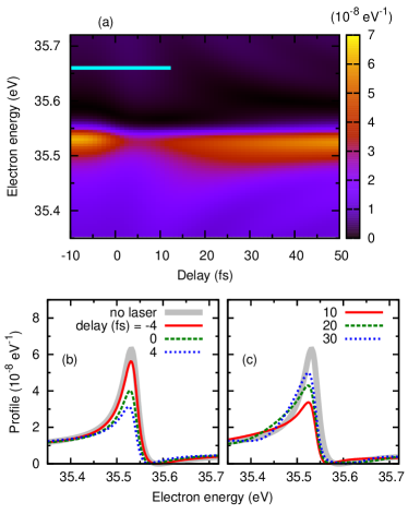
Figure 3: (Color online) Photoelectron profile of the $2s2p$ resonance for $\lambda_{L}=780$ nm. (a) The spectrogram. The cyan bar indicates the range of delay where the two pulses overlap. (b) The spectra for various $t_{0}$, and the case without laser.

Figure 4 shows the $2p^{2}$ resonance profiles. The signal is large in the range from $t_{0}=-10$ fs to 0 and low for $t_{0}>15$ fs. Starting from the left end of the spectrogram, for $t_{0}=-4$ fs, the tail part of the laser pulse is involved in the dynamics; counting only this involved part of the laser, the strength is low and the duration is short, and the Rabi oscillation is slow. As a result, the maximum population pumped to $2p^{2}$ is “trapped” without returning back to $2s2p$. At the same time, the ionization rate by this laser “tail” is low and not influential. The high population of the $2p^{2}$ state is shown in Fig. 2(b). At large time, it decays into the biggest photoelectron profile shown in Fig. 4(b). Moving on to $t_{0}=2$ fs, the laser strikes $2s2p$ mainly at the beginning of decay. As shown in Fig. 2(b), the full strength of laser depletes the population almost completely; at the end of laser, the $2p^{2}$ bound state is almost empty, and there are hardly any electrons to autoionize. Consequently, the $2p^{2}$ profile in Fig. 4 is greatly depressed, forming a valley in the spectrogram.

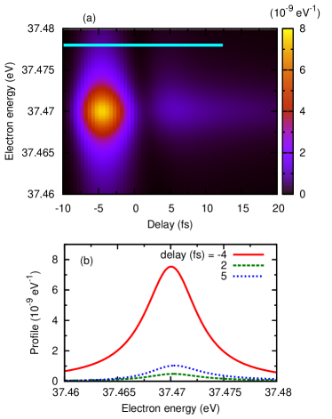
Figure 4: (Color online) As Fig. 3 but for the $2p^{2}$ resonance.

Note that the $2s2p$ and the $2p^{2}$ resonances are in different symmetries. Their momentum (or angular) distributions are different, but their energy ranges overlap because of the broad bandwidth of the SAP. If the momentum spectrum is measured, one can distinguish the contributions from the two resonances and separate out the spectra. However, if only the energy spectrum is measured, the two contributions are not separable near 37.5 eV, where the $2s2p$ resonance lies on the $1s\epsilon p$ background. The $1s\epsilon p$ background at 37.5 eV is $7.5\times 10^{-9}$ eV^-1, which is about the same as the peak value of the $2p^{2}$ profile shown in Fig. 4. The $2p^{2}$ resonance profile in the total energy spectrum will appear flatter than how it would look without the background.

The mechanism of the dressing laser is further analyzed when the calculations are done for various laser intensities. The curves in Fig. 5(a) and (b) represent the spectra for fixed delays but different intensities, where the medium one ($I_{L}=0.7$ TW/cm²) repeats the experimental condition. The delays 30 and 5 fs are chosen for $2s2p$ and $2p^{2}$ respectively for adequate signal strengths. For $2s2p$, with the increase of $I_{L}$, the profile gradually depresses and forms interference patterns. It suggests that if the laser at about 30 fs is strong enough, it will suddenly deplete the bound states and halt the decay process. The resultant profile is then constructed by the electrons autoionized before 30 fs. Fig. 5(a) also shows that the resonance peak moves gradually to the low-energy side with increasing IR coupling strength. For the $2p^{2}$ resonance shown in Fig. 5(b), increasing $I_{L}$ mainly populates more $2p^{2}$ and makes the profile larger.

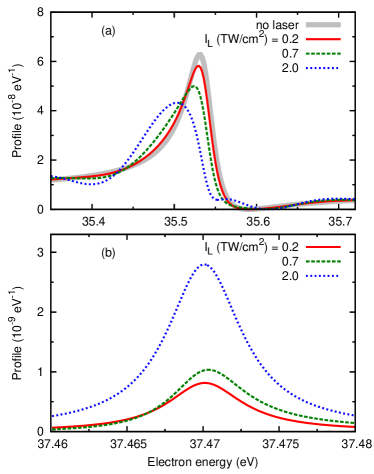
Figure 5: (Color online) Photoelectron profiles for $\lambda_{L}=780$ nm and various $I_{L}$, of (a) the $2s2p$ resonance for $t_{0}=30$ fs, and (b) the $2p^{2}$ resonance for $t_{0}=5$ fs.

III.1.2 Comparison with experiment

The experiment by Gilbertson et al gilbertson reported the spectrogram in the energy range 33–46 eV, enclosing both resonances in our concern. However, the energy resolution is insufficient for the very narrow $2p^{2}$ resonance with $\Gamma_{b}=5.9$ meV, making its transient spectra invisible. The most dominant feature in the spectrogram is the variation in peak height of $2s2p$ resonance, where the decay lifetime 17 fs can be extracted. In Fig. 6, the normalized peak value is shown as a function of $t_{0}$. The peak value for the most negative delay, which represents the “XUV only” case, is normalized to 1. The present calculation is displayed in three different settings, where the model excludes the laser ionization, includes the laser ionization from $2s2p$, and includes the laser ionization from both states. While the experiment did not know the absolute times of the pulses thus unable to determine the absolute delay, the experimental data is shifted by 4.5 fs to fit our calculation. In Fig. 6, the calculation result without laser ionization exhibits the similar decay feature found in the experiment, but the absolute value is too high. By adding the laser ionization, we are able to adjust the parameters such that the calculation agrees with the experiment quantitatively. The empirical ionization parameters are $C_{l}=0.5$ and $\alpha=0$ for $2s2p$ and $C_{l}=0.5$ and $\alpha=11$ for $2p^{2}$, where $C_{l}$ is defined in the PPT model ppt and $\alpha$ is defined in the correction term tong05 .

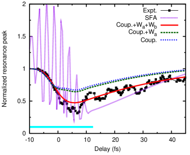
Figure 6: (Color online) The normalized peak value of the $2s2p$ profile as a function of delay for $\lambda_{L}=780$ nm. The value for $t_{0}=-10$ fs is set as 1. The present calculations are shown in three different settings where the ionization rates $W_{a}(t)$ and $W_{b}(t)$ are included or excluded. The experimental curve gilbertson is shifted in $t_{0}$ by 4.5 fs to fit the full calculation shown by the red solid curve. The result by the SFA model zhao is normalized such that it fits the experimental data the most. The cyan bar indicates the delay range where the two pulses overlap.

The comparison shown above indicates that the presence of the $2p^{2}$ state is responsible for the significant depression of the Fano peak, where both the coupling and the IR ionization take credit. The agreement between our model and the experiment is very good when both effects are taken into account. However, there are irregular oscillations in the experimental data; their period is typically between 5 and 10 fs, but mostly unpredictable. Their appearance is unexplained so far, but could be due to experimental artifact.

The experimental report included a simulation using the ”streaking” model (within the SFA) for isolated autoionizing states zhao , with the inclusion of ionization due to the laser calculated within the PPT model ppt , as described by Eq. 1 in Ref. gilbertson . In the SFA model, the ionization of $2s2p$ and the acceleration of the scattered electrons are treated separately, and the laser coupling to other bound or resonance states is totally disregarded. The common mechanism between the model therein and our model is that the laser ionization is treated by the PPT calculation. In order to have a clear view on the two approaches, we have reproduced the angular-differential electron spectrogram at the polarization direction, where the measurement was done, using the SFA model with the same parameters taken in our model. The result is shown in Fig. 7. The corresponding resonance peak is plotted in Fig. 6 which is normalized to fit the overall experimental data. The SFA results in Fig. 6 and in Fig. 7 are similar to our calculation for $t_{0}>10$ fs; the resonance peak goes through the same depression before the gradual revival along $t_{0}$. However, for $t_{0}<10$ fs, the strong streaking peaks carrying the laser period 2.6 fs are missing both in the experiment and in our model. This suggests that with the inclusion of coupling and ionization of $2p^{2}$, the present model takes charge of the primary effects seen in the time-delayed measurement. We comment that even though both the SFA model and the present one account for the ionization by the IR laser, it is the ionization of $2p^{2}$ that is mostly responsible for the great reduction in the resonance strength observed in the experiment. This state was not included in the SFA model.

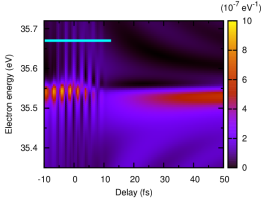
Figure 7: (Color online) The angular-differential spectrogram of the $2s2p$ resonance in the direction of the laser polarization calculated by the SFA model zhao .

The experiment also measured the spectrograms with several other laser intensities, and reported the depth of the “dip” that is seen in Fig. 6’s curve against $I_{L}$. The experimental and theoretical dip values are shown in Fig. 8. As seen in the figure, increasing $I_{L}$ will aggravate the depression of the resonance. The experimental dip is also deeper than the theoretical one for high $I_{L}$, i.e., the resonance peak is more depleted than what the present theory predicts. This is because as $I_{L}$ increases, the nonlinear interaction of the IR opens up more excitation and ionization pathways that deplete the $2s2p$ part (or the bound part) of the resonance. The depletion will lead to fewer autoionization events and thus weaker electron signal near the resonance. Note that the discrepancy between the present model and experimental data in Fig. 8 grows nonlinearly with $I_{L}$ for $I_{L}>4.5\times 10^{11}$ W/cm².

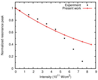
Figure 8: (Color online) The normalized peak value of the $2s2p$ profile at the dip (see text) as a function of the peak intensity of laser.

III.2 Laser wavelength of 540 nm

Using long pulses and laser spectroscopy, Autler-Townes doublet autler ; fleischhauer has been observed when two bound states are strongly coupled by a dressing laser field. For the two autoionizing states and the ultrashort laser in the present study, can we observe anything resembling the Autler-Townes doublet in the spectra? In Sec. III.1, we have shown that for the 780 nm IR, since the laser detuning is large and the laser ionization is significant, the evidence of Autler-Townes doublets is not prevalent except that the small shift of the $2s2p$ peak at higher coupling intensity in Fig. 5(a) gives a feeble hint. Now, we intentionally tune the laser to $\lambda_{L}=540$ nm (mean photon energy is 2.30 eV) so that it is in resonance between $2s2p$ and the lower-energy state, $2s^{2}(^{1}S)$ at $57.85$ eV. In this setup, first of all, the laser detuning is negligible, making the Rabi oscillation the strongest. Secondly, the binding energy of the $|b\rangle$ state changes from 3.34 eV for $2p^{2}$ to 7.55 eV for $2s^{2}$, which effectively shuts down its laser ionization. As a consequence, the Rabi flopping dominates, and other complications are minimized. Below we examine whether we can observe the Autler-Townes doublet for such a ”three-level system” where the two fast-decaying ”levels” are strongly coupled by a short pulse.

For the parameters in the model, the $2s^{2}$ resonance width ($\Gamma_{b}$) of 0.125 eV, or the lifetime of 5.3 fs, is taken from the earlier calculation chung . The dipole transition and the $q$-parameter are assumed to be the same as those for $2p^{2}$, i.e., $D_{ba}=2.17$ a.u. and $q_{b}=1000$, because the first-order transition in $D_{ba}$ is again $\langle 2s|D|2p\rangle$, and $D_{2a}$ has no first-order term. The PPT rate for $2s^{2}$ at the laser peak is in the order of 10^-5 eV which is negligible for our purpose. The Rabi frequency between $2s2p$ and $2s^{2}$ is 0.27 eV, corresponding to the period of 15 fs.

The evolution of the bound states is shown in Fig. 9. An obvious difference from the $\lambda_{L}=780$ nm case is that the laser coupling now is strong enough to completely deplete $2s2p$ so that its population almost touches zero before bouncing back, as shown in Figs. 9(b-d). However, when it revives, the amount brought back by the oscillation is only less than 10% of what has been removed. For the $2s^{2}$ state for $t_{0}=5$, 10, and 20 fs, the overall population decreases with the delay because the $2s2p$ decays with time and the laser pumps less and less electrons from $2s2p$ to $2s^{2}$.

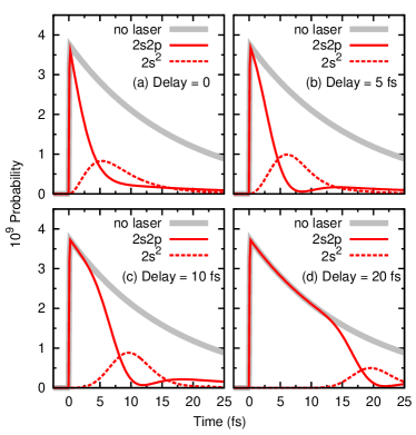
Figure 9: (Color online) Probabilities of the $2s2p$ and $2s^{2}$ bound states with time for $\lambda_{L}=540$ nm and various delays. The gray solid curve indicates the laser-free decay of $2s2p$.

Now we turn to the electron spectra of the $2s2p$ resonance in Fig. 10. When the delay passes the origin and becomes positive, the resonance profile flips horizontally, looking like the mirror image of the “no laser” spectrum other than an overall reduction in height. This flipped peak is seen in the $t_{0}=5$ fs curve in Fig. 10(c). To understand this pattern, in Fig. 9(b), the sharp drop of $2s2p$ from 0 to 7 fs suggests that most electrons move from $2s2p$ to $2s^{2}$ at the very beginning of the decay of $2s2p$. The laser duration allows the Rabi oscillation to run a little more than half cycle, which bounces only a small fraction of the population back to $2s2p$. The relatively few electrons returning to $2s2p$ have changed the phase by $\pi$ through this Rabi flopping, thus reversing the sign of $q$ in the resonance profile (See Ref. fano ). When $t_{0}$ increases, in Fig. 10(a), an additional ridge moves from the lower energy to the original peak position, stretching from 35.4 eV at $t_{0}=15$ fs to 35.5 eV at $t_{0}=50$ fs. This suggests that the laser divides the autoionization into two periods of time; the part prior to the laser is responsible for the regular Fano profile as shown by the “no laser” curve, and the part after the laser is responsible for the “inverse” shape that we have just discussed. Different delay times determine the fractions of these two parts, and the ridge forms at different energies as the interference pattern. Figure 10(d) clearly shows the shifting of the ridge while the inverse peak stays at 35.55 eV.

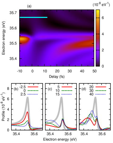
Figure 10: (Color online) As Fig. 3 but for $\lambda_{L}=540$ nm. The gray solid curve represents the “no laser” case.

The $2s^{2}$ profile in Fig. 11(a) has a very gentle and monotonic attenuation along $t_{0}$, while the $2p^{2}$ profile in Fig. 4(a) features a “gap” in $t_{0}$ where the profile drops to zero altogether before it regains some strength as $t_{0}$ increases. This gap, as explained in Sec. III.1.1, originates from the IR ionization; however in the $\lambda_{L}=540$ nm case, this mechanism is missing since the ionization rate for $2s^{2}$ is low. Rabi oscillation and autoionization are the only influences on the evolution of $2s^{2}$. Since the Rabi oscillation runs only a little more than half cycle, it can be viewed as a “one way route” for electrons from $2s2p$ to $2s^{2}$. Once arriving at $2s^{2}$, the electrons autoionize quickly to form the $2s^{2}$ profile. As $t_{0}$ increases, more electrons will autoionize from $2s2p$ and less will be brought by the laser to $2s^{2}$, and the $2s^{2}$ resonance becomes weaker.

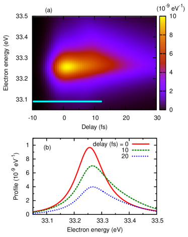
Figure 11: (Color online) As Fig. 10 but for the $2s^{2}$ resonance.

The choice of $2s^{2}$ as the second coupled state is optimal for practical measurement issues, such as the signal strength and energy resolution. One must remember that the $2s^{2}$ resonance is on top of the $1s\epsilon p$ background if the total electron energies are measured. The maximum signal intensity of the $2s^{2}$ profile is nearly 10^-8 eV^-1, and the nearby $1s\epsilon p$ background is $7.5\times 10^{-9}$ eV^-1, i.e., when the two are layered together, the resonance signal is high enough to stand out from the background. Furthermore, its resonance width $\Gamma_{b}=0.125$ eV is larger than that of $2s2p$, making its visibility better even with the same energy resolution used in Ref. gilbertson . Considering both the height and the width in spectrum, detecting the $2s^{2}$ resonance vs delay should be feasible.

The complicatedly structured profiles seen in Figs. 10(b-d) are in contrast to the Autler-Townes doublet in long-pulse cases. The latter features the splitting proportional to the field strength, and each peak in the doublet does not differ from the original single peak in shape. In order to clarify the difference between long and short pulses in a systematic way, in Fig. 12, we show what the $2s2p$ profile should look like if the laser is 1 ps long, with all other parameters unchanged. A 1 ps laser pulse is much longer than our atomic time scale and equivalent to a stable AC field, where time delay cannot be defined. The separation of the splitting is about the Rabi frequency 0.27 eV. Nevertheless, in a standard EIT setup, the $|b\rangle$ state is a bound state, which is not the case in the present system. As a result, in our example, the split peaks are fainter because of the finite lifetime of $2s^{2}$.

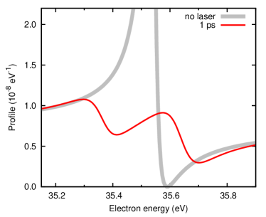
Figure 12: (Color online) Photoelectron profile of the $2s2p$ resonance with a 540 nm, 1 ps laser pulse. The original Fano line-shape is plotted in the gray solid curve.

If the laser duration shrinks from 1 ps to 50 fs, the magnitude of the splitting will be a function of the time delay. However, since the laser is still significantly longer than the 17 fs decay lifetime in concern, the delay-dependence is more relevant to the overlap between the pulses rather than the autoionization. This scenario has been studied with transient absorption spectroscopy in helium where the XUV is 30 fs and the IR is 42 fs loh . The study showed that the splitting was tuned to maximum by overlapping the pulses, and it disappeared when the pulses were totally separate. The system can be viewed as a dressed atom where the dressing condition can be slowly turned on or off by changing the time delay.

As the comparison indicates, the mechanisms for the short and long pulses are indeed very different. For a long dressing pulse, the field enters as the coupling (off-diagonal) terms in the Hamiltonian of the system. When the Hamiltonian is diagonalized, the energy levels are shifted, which are then represented by the doublet. However, for a short dressing pulse, the coupling strength changes quickly; the Rabi frequency is not well-defined, and the mechanism for the long pulse breaks down. In other words, the dressing field influences only a short temporal segment out of the whole autoionization, while most of the time, the resonance profile evolves without laser and aims at the single-peak Fano profile rather than the doublet.

IV Summary and Conclusions

A model has been developed to study the autoionization dynamics in a laser-dressed helium. An attosecond XUV excites the $2s2p$ resonance in a time-delayed 780 nm IR pulse. The IR can couple the $2s2p$ and $2p^{2}$ states and ionize the two states. The photoelectron energy spectra for different time delays are calculated and compared with the experiment gilbertson . While the experimental energy resolution was not good enough to observe the resonance shape in detail, good agreement for the resonance peak intensity vs time delay between our model and the experiment has been achieved. The decay lifetime of $2s2p$ can be retrieved by this result. Because of the strong IR ionization, the coupling with $2p^{2}$ is to open an efficient pathway where the $2s2p$ resonance can be depleted, i.e., the IR field modifies the profile with an overall depression without changing the spectral shape, which is totally different from the typical three-level systems.

To reduce the effect of ionization by the IR laser, we change the laser wavelength to 540 nm and consider the coupling of the $2s2p$ and $2s^{2}$ states. The $2s^{2}$ state has a larger binding energy where its ionization is negligible. In this case, a complicated pattern in the $2s2p$ resonance shape vs time delay has been found. The result is interpreted by the Rabi oscillation between the two autoionizing states whose cycles are confined by the 9 fs laser. In order to make connection of this result to the traditional dressed-atoms, we change the laser duration to 1 ps and recover the Autler-Townes splitting in the spectrum, which also clarifies the difference between the short- and long-dressing fields. In order words, in the presence of an intense IR, autoionization dynamics can be changed significantly. The possibilities of such manipulations are tremendous, and what one can gain from such experiments remains to be further explored.

- (1) F. Krausz and M. Ivanov, Rev. Mod. Phys. 81, 163 (2009).
- (2) X. M. Tong, P. Ranitovic, C. L. Cocke, and N. Toshima, Phys. Rev. A 81, 021404(R) (2010).
- (3) F. Kelkensberg et al, Phys. Rev. Lett. 103, 123005 (2009).
- (4) F. Kelkensberg et al, Phys. Rev. Lett. 107, 043002 (2011).
- (5) Sansone et al, Nature 465, 763 (2010).
- (6) P. Johnsson, J. Mauritsson, T. Remetter, A. L’Huillier, and K. J. Schafer, Phys. Rev. Lett. 99, 233001 (2007).
- (7) P. Ranitovic et al, New J. Phys. 12, 013008 (2010).
- (8) P. Ranitovic, X. M. Tong, C. W. Hogle, X. Zhou, Y. Liu, N. Toshima, M. M. Murnane, and H. C. Kapteyn, Phys. Rev. Lett. 106, 193008 (2011).
- (9) J. Mauritsson et al, Phys. Rev. Lett. 105, 053001 (2010).
- (10) N. Shivaram, A. Roberts, L. Xu, and A. Sandhu, Opt. Lett. 35, 3312 (2010).
- (11) N. N. Choi, T. F. Jiang, T. Morishita, M.-H. Lee, and C. D. Lin, Phys. Rev. A 82, 013409 (2010).
- (12) M. Holler, F. Schapper, L. Gallmann, and U. Keller, Phys. Rev. Lett. 106, 123601 (2011).
- (13) M. B. Gaarde, C. Buth, J. L.Tate, and K. J. Schafer, Phys. Rev. A 83, 013419 (2011).
- (14) M. Kitzler, N. Milosevic, A. Scrinzi, F. Krausz, and T. Brabec, Phys. Rev. Lett. 88, 173904 (2002).
- (15) Y. Mairesse and F. Quéré, Phys. Rev. A 71, 011401(R) (2005).
- (16) R. P. Madden and K. Codling, Phys. Rev. Lett 10, 516 (1963).
- (17) M. Domke et al, Phys. Rev. Lett 66, 1306 (1991).
- (18) M. Drescher et al, Nature 419, 803 (2002).
- (19) U. Fano, Phys. Rev. 124, 1866 (1961).
- (20) W.-C. Chu and C. D. Lin, Phys. Rev. A 82, 053415 (2010).
- (21) M. Wickenhauser and J. Burgdörfer, Laser Phys. 14, 492 (2004).
- (22) Z. X. Zhao and C. D. Lin, Phys. Rev. A 71, 060702R (2005).
- (23) Z.-H. Loh, C. H. Greene, and S. R. Leone, Chem. Phys. 350, 7 (2008).
- (24) S. Gilbertson et al, Phys. Rev. Lett. 105, 263003 (2010).
- (25) P. Lambropoulos and P. Zoller, Phys. Rev. A 24, 379 (1981).
- (26) H. Bachau, P. Lambropoulos, and R. Shakeshaft, Phy. Rev. A 34 4785 (1986).
- (27) L. B. Madsen, P. Schlagheck, and P. Lambropoulos, Phys. Rev. Lett. 85, 42 (2000).
- (28) S. I. Themelis, P. Lambropoulos, and M. Meyer, J. Phys. B: At. Mol. Opt. Phys. 37, 4281 (2004).
- (29) S. E. Harris, Phys. Rev. Lett. 62, 1033 (1989).
- (30) M. Fleischhauer, A. Imamoglu, and J. P. Marangos, Rev. Mod. Phys. 77, 633 (2005).
- (31) S. H. Autler and C. H. Townes, Phys. Rev. 100, 703 (1955).
- (32) C. D. Lin, Adv. At. Mol. Phys. 22, 77 (1986).
- (33) M. Domke, K. Schulz, G. Remmers, G. Kaindl, and D. Wintgen, Phys. Rev. A 53, 1424 (1996).
- (34) A. Burgers, D. Wintgen, and J.-M. Rost, J. Phys. B: At. Mol. Opt. Phys. 28, 33163 (1995).
- (35) A. M. Perelomov, V. S. Popov, M. V. Terent’ev, Sov. Phys. JETP 23, 924 (1966); 24, 207 (1967).
- (36) X. M. Tong and C. D. Lin, J. Phys. B: At. Mol. Opt. Phys. 38, 2593 (2005).
- (37) K. T. Chung and B. F. Davis, Phys. Rev. A 26, 3278 (1982).