Upper transition point for percolation on the enhanced binary tree: A sharpened lower bound

Abstract

Hyperbolic structures are obtained by tiling a hyperbolic surface with negative Gaussian curvature. These structures generally exhibit two percolation transitions: a system-wide connection can be established at a certain occupation probability $p=p_{c1}$ and there emerges a unique giant cluster at $p_{c2}>p_{c1}$. There have been debates about locating the upper transition point of a prototypical hyperbolic structure called the enhanced binary tree (EBT), which is constructed by adding loops to a binary tree. This work presents its lower bound as $p_{c2}\gtrsim 0.55$ by using phenomenological renormalization-group methods and discusses some solvable models related to the EBT.

I Introduction

Percolation has been one of the most popular model systems in statistical physics and it still remains as an active research area. For a classical introduction, one may refer to Refs. Stauffer and Aharony (1994); Grimmett (1999). One recent observation in this field is that there generally occur two percolation transitions if the size of a given system expands exponentially fast as its length scale grows. For example, the size of a binary tree increases as $N\sim 2^{L}$ with the number of layers $L$ [Fig. 1(a)]. At the first percolation point $p^{\rm tree}_{c1}=1/2$, it becomes possible to establish a global connection, and the resulting cluster size scales linearly with $L$. However, this cluster size is still negligible compared with $N$ since $L/2^{L}\rightarrow 0$ as $L$ increases. We find the largest cluster size $s_{1}$ comparable to $N$ only at $p=1$, which determines $p^{\rm tree}_{c2}=1$. This tree in fact belongs to a category called hyperbolic lattices, obtained by tessellating a hyperbolic surface appearing in hyperbolic geometry. Since such double percolation transitions in hyperbolic structures were revealed by numerical calculations Baek et al. (2009a), there have been debates about locating the upper transition point Nogawa and Hasegawa (2009); Baek et al. (2009b); Minnhagen and Baek (2010); Baek and Minnhagen (2011a), particularly by dealing with a prototypical lattice model called the enhanced binary tree (EBT). This structure is not a tree in itself, but is derived from the binary tree by connecting vertices on the same layer horizontally [Fig. 1(b)]. It thus describes spreading along a branching structure with possible horizontal transfer. While the duality relation implies $p_{c2}=0.564(1)$ Nogawa and Hasegawa (2009), we have obtained $p_{c2}\approx 0.5$ by utilizing a simple extrapolation of the largest cluster size $s_{1}\sim N^{-\phi}$, which is correct for a tree Baek et al. (2009a). This looks also consistent with the observation of $s_{2}/s_{1}$ where $s_{2}$ is the size of the second largest cluster Baek et al. (2009b). We have even tried to explain this estimate $p_{c2}=1/2$ analytically in combination with numerical observations and approximate renormalization-group methods Minnhagen and Baek (2010); Baek and Minnhagen (2011a), pointing out that the duality argument does not have a solid mathematical ground here.

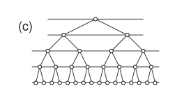
Figure 1: (a) Schematic representations of a simple binary tree and (b) of the EBT derived from (a). These are drawn on the Poincaré disk, where the circular boundary indicates points at infinity. (c) A part of the EBT.

Recently, Ref. Gu and Ziff revisited this issue by calculating the crossing probability. According to the conformal field theory Cardy (1992), the crossing probability for a unit disk whose boundary is divided at four points $z_{1},z_{2},z_{3}$ and $z_{4}$ is given by

$$R=\frac{\Gamma(\frac{2}{3})}{\Gamma(\frac{4}{3})\Gamma(\frac{1}{3})}\eta^{\frac{1}{3}}~{}_{2}F_{1}(\frac{1}{3},\frac{2}{3};\frac{4}{3},\eta),$$ (1)

with the gamma function $\Gamma$, the hypergeometric function ${}_{2}F_{1}$, and the cross ratio

$$\eta=\frac{(z_{1}-z_{2})(z_{3}-z_{4})}{(z_{1}-z_{3})(z_{2}-z_{4})}.$$

If the boundary is divided into four equal pieces, e.g., $z_{1}=-1$, $z_{2}=-i$, $z_{3}=1$, and $z_{4}=i$, the cross ratio becomes $\eta=1/2$ and we immediately find $R=1/2$ (see, e.g., Refs. Kleban and Vassileva (1994); Rietman et al. (1992) on the connection between the hyperbolic geometry and the conformal field theory). Such a point where $R=1/2$ is denoted as a duality point in Ref. Gu and Ziff . For each of several hyperbolic structures considered there, they have numerically calculated $R(p)$ by dividing the boundary into four equal intervals. Then by extrapolating $R(p)$ to the large-size limit at the inflection point, Ref. Gu and Ziff suggests that the limiting tangent line gives an upper bound of $p_{c1}$ and a lower bound of $p_{c2}$. A notable point is that the slope of the line converges to a finite value, which clearly differs from the two-dimensional (2D) results. This method yields $p_{c2}\geq 0.503$ for the EBT, questioning the validity of the claim that $p_{c2}=1/2$. They have also estimated $p_{c2}$ as $0.564(10)$ by extrapolating the value of $p$ where $R(p)=1-\epsilon$ with $\epsilon\ll 1$ as growing the system size, which is consistent with the estimate in Ref. Nogawa and Hasegawa (2009). In this paper, equipped with better analytic tools than before, we too reach a conclusion that $p_{c2}$ is indeed larger than $1/2$. Our new lower bound, $p_{c2}\gtrsim 0.55$, is obtained by transfer-matrix calculations for percolation and includes the lower bound in Ref. Gu and Ziff .

This paper is organized as follows. In Sec. II, we consider two solvable models. Even though both of them have the trivial transition point $p_{c2}=1$, this consideration gives an insight about percolation in the EBT. Then in Sec. III, we deal with the EBT in two different ways: one is the block-cell transformation and the other is the transfer-matrix method. Both of them lead to $p_{c2}>1/2$ but the latter gives a sharper bound. We then conclude this work by reexamining our previous estimate in Sec. IV.

II Solvable models

II.1 Ternary tree

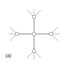
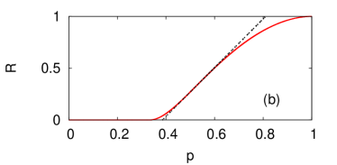
Figure 2: (Color online) (a) Schematic representation of a ternary tree. (b) Crossing probability $R$ given by Eq. (2) with a tangent line at the inflection point $p\approx 0.524~{}032$ (dotted line).

A tree with coordination number $g=4$ is the simplest example to calculate the crossing probability. The coordination number is chosen to provide the structure with natural four-fold symmetry. The center node has four branches [solid lines in Fig. 2(a)], each of which leads to a tree with branching ratio $b=g-1=3$ [dotted lines in Fig. 2(a)]. Inside each tree, the probability $\psi$ to connect the top to the boundary can be described by the Galton-Watson process Williams (1991), where the extinction probability $w$ can be identified with $1-\psi$. The number of offsprings $k$ for each node is chosen from a binomial distribution $B(3,p)$, where $p$ is the occupation probability of each bond. The generating function is readily obtained as $\phi(s)\equiv\sum_{k=0}^{\infty}s^{k}\binom{3}{k}p^{k}(1-p)^{3-k}=(1-p+sp)^{3}$. The extinction probability is then given by a solution of the equation $\phi(w)=w$ Williams (1991), which is

$$w=\left\{\begin{array}[]{lc}1&\mbox{if~{}}0\leq p\leq\frac{1}{3}\\ \frac{-3p^{2}+2p^{3}+\sqrt{4p^{3}-3p^{4}}}{2p^{3}}&\mbox{if~{}}\frac{1}{3}\leq p\leq 1,\end{array}\right.$$

or, equivalently,

$$\psi=\left\{\begin{array}[]{lc}0&\mbox{if~{}}0\leq p\leq\frac{1}{3}\\ \frac{3p^{2}-\sqrt{4p^{3}-3p^{4}}}{2p^{3}}&\mbox{if~{}}\frac{1}{3}\leq p\leq 1.\end{array}\right.$$

If we also consider the probability to connect two opposite branches of the central cross in Fig. 2(a), we get the crossing probability as

$$R(p)=2p^{2}(1-p)^{2}\psi^{2}+4p^{3}(1-p)\psi^{2}+p^{4}[2\psi^{2}(1-\psi)^{2}+4\psi^{3}(1-\psi)+\psi^{4}],$$ (2)

where $2p^{2}(1-p)^{2}$, $4p^{3}(1-p)$, and $p^{4}$ describe the connecting configurations of the central cross and the other $\psi$-dependent parts describe configurations of the trees attached to the cross. One should note that we have considered crossing in either direction, while it is in only one given direction in Eq. (1) and Ref. Gu and Ziff . This difference in the definition of crossing will not change any essential behavior, however. We plot the result in Fig. 2(b), and an interesting point is that the slope of this function is finite everywhere between $p_{c1}=1/3$ and $p_{c2}=1$, in accordance with the numerical analysis in Ref. Gu and Ziff . Note that this is markedly different from the 2D percolation where the slope diverges at the critical point. We also see that the tangent line at the inflection point $p\approx 0.524~{}032$ does give a lower bound of $p_{c2}$ as well as an upper bound of $p_{c1}$ as suggested in Ref. Gu and Ziff .

II.2 Binary tree with a ring at the boundary

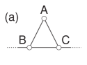
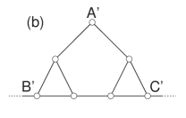
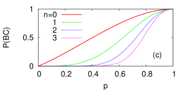
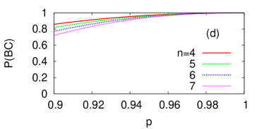
Figure 3: (Color online) Binary tree with a ring at the boundary. (a),(b) Probabilities of connection in $\triangle ABC$ determine those in $\triangle A^{\prime}B^{\prime}C^{\prime}$, resulting in the recursion Eq. (3). (c) The probability of connection between two farthest points on the boundary, $P(BC)$, when the recursion equation is iterated $n$ times. (d) The same quantity for $p\geq 0.9$ with $n=4,\ldots,7$.

Let us add loops to a tree by attaching a ring along the boundary points. This may be regarded as a first step toward making the EBT, and even this single ring can introduce a large number of loops into the system. We first focus on the smallest triangle touching the boundary and denote it as $\triangle ABC$ [Fig. 3(a)]. Following Ref. Ziff (2006), we define $P(ABC)$ as the probability that all the three points are connected to one another, while $P(\bar{A}\bar{B}\bar{C})$ as the probability that there is no connection among them. In addition, $P(\bar{A}BC)$ means the probability that $B$ and $C$ are connected but $A$ is not. One can also define $P(A\bar{B}C)$ and $P(AB\bar{C})$ in the same way. These cover the whole possibilities by

$$P(ABC)+P(\bar{A}\bar{B}\bar{C})+P(\bar{A}BC)+P(A\bar{B}C)+P(AB\bar{C})=1.$$

Considering a larger triangle $\triangle A^{\prime}B^{\prime}C^{\prime}$ containing the two smallest triangles [Fig. 3(b)], we find that it is possible to express the five probabilities of $\triangle A^{\prime}B^{\prime}C^{\prime}$ with those of $\triangle ABC$. Note that the left-right symmetry is preserved by this transformation so that we have three independent variables $x\equiv P(ABC)$, $y\equiv P(\bar{A}BC)$, and $z\equiv P(A\bar{B}C)$. After some algebra, the transformation turns out to be

$$x^{\prime} = p^{2}(z^{2}+2xz+2xy-2px^{2}+3x^{2}),$$

$$y^{\prime} = p(y-px+x)^{2},$$ (3)

$$z^{\prime} = -p(pz^{2}-pyz+p^{2}xz+pxz-z+pxy-p^{2}x^{2}+2px^{2}-x),$$

where the prime is in order to indicate probabilities for $\triangle A^{\prime}B^{\prime}C^{\prime}$. The initial condition is given by counting the possibilities in $\triangle ABC$ as

$$x = p^{3}+3p^{2}(1-p),$$

$$y = p(1-p)^{2},$$

$$z = p(1-p)^{2}.$$

The quantity of interest is $P(BC)=P(ABC)+P(\bar{A}BC)=x+y$, and this can be obtained exactly at every iteration step [Fig. 3(c)]. Note that this quantity is closely related to the crossing probability since it measures the chance for a boundary point to connect to another boundary point far away, which is possibly achieved through the inner part of the system. When this transformation is iterated, we observe that $P(BC)$ eventually vanishes except at $p=1$ [Fig. 3(c)], so we conclude that the added loops are not enough to make $p_{c2}$ nontrivial. However, it is notable that the convergence is so slow that it is hard to determine $p_{c2}$ by naive extrapolation [Fig. 3(d)].

III Enhanced binary tree

III.1 Block-cell transformation

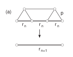
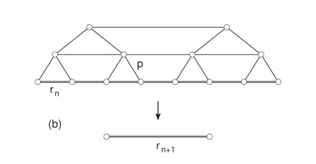
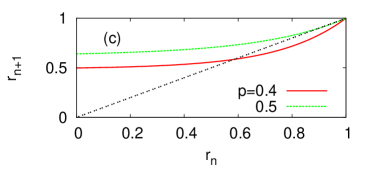
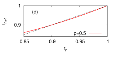
Figure 4: (Color online) (a) Block-cell transformation for eight bonds, where $r_{n}$ is the renormalized connection probability at the $n$-th iteration step, represented by double lines. (b) Transformation for 23 bonds and (c) its application at $p=0.4$ and $0.5$. The dotted line indicates a slope of $1$. (d) A zoomed view at $p=0.5$ shows that this $p$ is still below $p_{c2}$.

The block-cell transformation shown in Fig. 4(a) was introduced to get a lower bound of $p_{c2}$ in Ref. Baek and Minnhagen (2011a). It yields a lower bound because we systematically overestimate connection at each transformation. Using this transformation in Fig. 4(a), we concluded $p_{c2}\geq 1/2$ Baek and Minnhagen (2011a), because the limiting connection probability $r_{\infty}$ became one for $p\geq 1/2$. Later in Ref. Baek and Minnhagen (2011b), it was pointed out that the same method was applicable to find lower bounds for the usual 2D percolation thresholds as well, and also that such a lower bound approached the true critical point $p_{c}$ as we used a larger block. For the square lattice, a small block already predicts the correct critical point of the bond percolation, $p^{\rm square}_{c}=1/2$, and using a larger block does not change this estimate, which can be an indication of the exactness of $p^{\rm square}_{c}=1/2$. This observation motivates us to take a larger block in the EBT [Fig. 4(b)], which requires us to check $2^{23}\approx 8\times 10^{6}$ configurations. The enumeration is straightforward with a personal computer and the result is as follows:

$$r_{n+1} = 9p^{12}r_{n}^{7}-91p^{11}r_{n}^{7}+409p^{10}r_{n}^{7}-1071p^{9}r_{n}^{7}+1795p^{8}r_{n}^{7}-1982p^{7}r_{n}^{7}+1414p^{6}r_{n}^{7}$$

$$-590p^{5}r_{n}^{7}+91p^{4}r_{n}^{7}+25p^{3}r_{n}^{7}-7p^{2}r_{n}^{7}-3pr_{n}^{7}+r_{n}^{7}-25p^{12}r_{n}^{6}+227p^{11}r_{n}^{6}$$

$$-904p^{10}r_{n}^{6}+2060p^{9}r_{n}^{6}-2928p^{8}r_{n}^{6}+2632p^{7}r_{n}^{6}-1414p^{6}r_{n}^{6}+354p^{5}r_{n}^{6}+25p^{4}r_{n}^{6}$$

$$-27p^{3}r_{n}^{6}-2p^{2}r_{n}^{6}+2pr_{n}^{6}+24p^{12}r_{n}^{5}-185p^{11}r_{n}^{5}+600p^{10}r_{n}^{5}-1038p^{9}r_{n}^{5}+969p^{8}r_{n}^{5}$$

$$-354p^{7}r_{n}^{5}-165p^{6}r_{n}^{5}+210p^{5}r_{n}^{5}-57p^{4}r_{n}^{5}-9p^{3}r_{n}^{5}+5p^{2}r_{n}^{5}-9p^{12}r_{n}^{4}+51p^{11}r_{n}^{4}$$

$$-102p^{10}r_{n}^{4}+60p^{9}r_{n}^{4}+60p^{8}r_{n}^{4}-70p^{7}r_{n}^{4}-46p^{6}r_{n}^{4}+92p^{5}r_{n}^{4}-35p^{4}r_{n}^{4}-5p^{3}r_{n}^{4}$$

$$+4p^{2}r_{n}^{4}+p^{12}r_{n}^{3}-2p^{11}r_{n}^{3}-24p^{9}r_{n}^{3}+115p^{8}r_{n}^{3}-198p^{7}r_{n}^{3}+150p^{6}r_{n}^{3}-32p^{5}r_{n}^{3}$$

$$-18p^{4}r_{n}^{3}+8p^{3}r_{n}^{3}-3p^{10}r_{n}^{2}+13p^{9}r_{n}^{2}-14p^{8}r_{n}^{2}-12p^{7}r_{n}^{2}+31p^{6}r_{n}^{2}-13p^{5}r_{n}^{2}$$

$$-6p^{4}r_{n}^{2}+4p^{3}r_{n}^{2}+3p^{8}r_{n}-16p^{7}r_{n}+31p^{6}r_{n}-26p^{5}r_{n}+8p^{4}r_{n}-p^{6}+5p^{5}$$

$$-8p^{4}+4p^{3}+p.$$

The system-wide connection probability $r_{\infty}$ grows as we increase $p$ [Fig. 4(c)]. By checking the value of $p$ where $r_{\infty}$ becomes $1$, we locate a lower bound of $p_{c2}$. In fact, a careful look shows that $p=1/2$ is still below $p_{c2}$ [Fig. 4(d)] and locates a sharper bound $p_{c2}\gtrsim 0.523$.

III.2 Transfer-matrix method

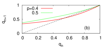
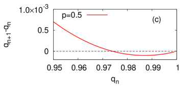
Figure 5: (Color online) (a) Unit cell for a transfer matrix calculation of a layer with width 1. Each bond at the bottom line has an occupation probability $q_{n}$ (represented by a double line), while the other bonds have an occupation probability $p$. (b) Iteration maps for $p=0.4$ and $0.5$. (c) $p=0.5$ has an intersection at $q_{\infty}<1$ and therefore lies below $p_{c2}$. The dotted lines indicate $q_{n+1}=q_{n}$.

In studying the Ising model on the EBT in Ref. Baek et al. (2011), we pointed out that the transfer-matrix method performed better than the block-cell transformation. Hence, we employ the transfer-matrix formalism developed for percolation in Ref. Derrida and Vannimenus (1980). First, we consider a unit cell of three spins as shown in Fig. 5(a). Note that a bond on the bottom line has a different probability of $q_{n}$ from the others with $p$. By attaching these cells from left to right, we construct an indefinitely long strip, or a layer of width $1$, which we can solve by using the transfer-matrix method. When we consider connection to the leftmost side, this cell has three possibilities: first, only the top point $A$ is connected (case 1), second, only $B$ is connected (case 2), or finally, both of them are connected (case 3). So we have nine possibilities of connection in total as follows:

$$P_{11}\equiv P(1\rightarrow 1) = p(p^{2}q_{n}^{2}-pq_{n}^{2}-pq_{n}+1),$$

$$P_{21}\equiv P(1\rightarrow 2) = pq_{n}(1-p)(1+q_{n}-pq_{n}),$$

$$P_{31}\equiv P(1\rightarrow 3) = p^{2}q_{n}(1+q_{n}-pq_{n}),$$

$$P_{12}\equiv P(2\rightarrow 1) = p^{2}(1-q_{n})(1+2q_{n}-2pq_{n}),$$

$$P_{22}\equiv P(2\rightarrow 2) = q_{n}(1-p)(p^{2}+q_{n}+pq_{n}-2p^{2}q_{n}),$$

$$P_{32}\equiv P(2\rightarrow 3) = p^{2}q_{n}(p+2q_{n}-2pq_{n}),$$

$$P_{13}\equiv P(3\rightarrow 1) = p(1-q_{n})(1+q_{n}-pq_{n}),$$

$$P_{23}\equiv P(3\rightarrow 2) = q_{n}(1-p)(p+q_{n}-pq_{n}),$$

$$P_{33}\equiv P(3\rightarrow 3) = pq_{n}(p+q_{n}-pq_{n}).$$

The global probability of connection to the leftmost side when $n(\gg 1)$ blocks are attached will behave as $\sim\lambda^{n}$, where $\lambda$ is the largest eigenvalue of this $3\times 3$ matrix $\{P_{ij}\}$. So we replace this layer by a one-dimensional chain, and identify its occupation probability $q_{n+1}$ with $\lambda$ to recover the original configuration in Fig. 5(a), but with $q_{n+1}$ instead of $q_{n}$. This iteration therefore determines $q_{n+1}$ as a function of $q_{n}$ and $p$, and we will find a limiting value $q_{\infty}=\lim_{n\rightarrow\infty}q_{n}$ for a large system. This renormalized connection probability is an increasing function of $p$ [Fig. 5(b)]. Again, we are interested in the value of $p$ making $q_{\infty}=1$, and such $p$ is found to be $\approx 0.504$. In short, this confirms that $p=1/2$ is strictly below $p_{c2}$ [Fig. 5(c)].

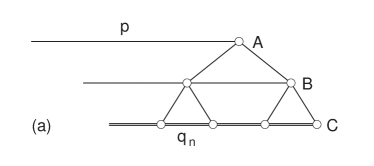
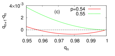
Figure 6: (Color online) (a) Unit cell for a transfer-matrix calculation of a layer with width $2$. (b) Ten possible cases of connection. A black dot means that it is connected to the leftmost side, and a white dot means it is not. A double circle means that these two are connected to each other, while none of them are connected to the leftmost side. (c) The resulting iteration map suggests a new lower bound of $p_{c2}$ as around $p=0.55$.

We can take a larger layer, expecting a sharper bound [Fig. 6(a)]. This consideration has ten possible cases as listed in Fig. 6(b). Here, the black dots are connected to the leftmost side while the white dots are not. It is important to consider possibilities that two white dots may be connected to each other since a percolating path may go backward for a while, so such dots are represented by double circles. In fact, the case indexed as $4$ is not accessible from any other states so it can be discarded. Each matrix element is expressed as a high-order polynomial, so the average number of terms per polynomial amounts to $18.4$. It is merely a mechanical procedure to obtain the matrix elements so we show only the final result with the largest eigenvalue, which is identified with $q_{n+1}$ as above. The result shown in Fig. 6(c) shows the highest lower bound of $p_{c2}$, which is around $p=0.55$. It includes the numerical lower bound suggested in Ref. Gu and Ziff and the estimate based on the duality relation Nogawa and Hasegawa (2009).

IV Discussion

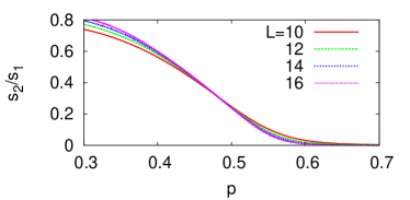
Figure 7: (Color online) Ratio of the second largest cluster size with respect to the largest cluster size in the EBT with different numbers of layers $L$. Our calculation suggests that the slope at $p=1/2$ will converge to a finite value in the large-$N$ limit.

At the time of writing Refs. Baek et al. (2009a, b), we assumed that the percolating properties in hyperbolic lattices could be inferred from known 2D results and also from the results of a tree. For example, $s_{2}/s_{1}$ has a diverging slope at the emergence of a giant cluster both for a 2D plane and for a tree. That is why we expected the same behavior for hyperbolic structures as well. However, as we see a clear difference from the 2D result in Fig. 2(b), such an assumption now looks quite dubious. Based on the results so far obtained, it seems more plausible that this ratio also has a constant slope at the large-$N$ limit (Fig. 7). This implies that percolation in the EBT is neither similar to its 2D counterpart nor to the percolation in a simple tree. In particular, we see that the competition between the largest and the second largest clusters appears milder than has been believed, so that $s_{2}/s_{1}$ may vanish smoothly around $p_{c2}$. In addition, it is inevitable to reconsider the phenomenological description of the critical phenomena around $p_{c2}$ by using scaling collapse Baek et al. (2009a) since it is likely that the critical points in the hyperbolic lattices have been generally underestimated. Our second example in Sec. II, however, suggests that it can be difficult to extract the critical behavior if one solely relies on numerical data. It will be interesting to challenge this problem by making use of the recent analytic approaches to hierarchical structures (see, e.g., Ref. Boettcher et al. (2009); Boettcher and Brunson (2011)).