The Distribution Of Metals in Cosmological Hydrodynamical Simulations of Dwarf Disk Galaxies

Abstract

We examine the chemical properties of five cosmological hydrodynamical simulations of an M33-like disc galaxy which have been shown previously to be consistent with the morphological characteristics and bulk scaling relations expected of late-type spirals. These simulations are part of the Making Galaxies In a Cosmological Context (MaGICC) Project, in which stellar feedback is tuned to match the stellar mass – halo mass relationship. Each realisation employed identical initial conditions and assembly histories, but differed from one another in their underlying baryonic physics prescriptions, including (a) the efficiency with which each supernova energy couples to the surrounding interstellar medium, (b) the impact of feedback associated with massive star radiation pressure, (c) the role of the minimum shut-off time for radiative cooling of Type II supernovae remnants, (d) the treatment of metal diffusion, and (e) varying the initial mass function. Our analysis focusses on the resulting stellar metallicity distribution functions (MDFs) in each simulated (analogous) ‘solar neighbourhood’ (2$-$3 disc scalelengths from the galactic centre) and central ‘bulge’ region. We compare and contrast the simulated MDFs’ skewness, kurtosis, and dispersion (inter-quartile, inter-decile, inter-centile, and inter-tenth-percentile regions) with that of the empirical solar neighbourhood MDF and local group dwarf galxies. We find that the MDFs of the simulated discs are more negatively skewed, with higher kurtosis, than those observed locally in the Milky Way and local group dwarfs. We can trace this difference to the simulations’ very tight and correlated age-metallicity relations (compared with that of the Milky Way’s solar neighbourhood), suggesting that these relations within ‘dwarf’ discs might be steeper than in L_⋆ discs (consistent with the simulations’ star formation histories and extant empirical data) and/or the degree of stellar orbital re-distribution and migration inferred locally has not been captured in their entirety, at the resolution of our simulations. The important role of metal diffusion in ameliorating the over-production of extremely metal-poor stars is highlighted.

1 Introduction

The relative number of stars of a given metallicity in a given environment, whether it be the local stellar disc, central spheroid/bulge, and or baryonic halo – the so-called metallicity distribution function (MDF) – has embedded within it, the time evolution of a system’s star formation, assembly/infall, and outflow history, all convolved with the initial mass function (IMF) (Tinsley, 1980). Seminal reviews of the diagnostic power of the MDF include those of Haywood (2001) and Caimmi (2008).

Well in advance of our now empirical appreciation of (a) the hierarchical assembly of galaxies from sub-galactic units, (b) the ongoing infall of fresh material from halos to discs (e.g. High-Velocity Clouds: Gibson et al. (2001)), and (c) the ongoing outflow of enriched material from discs via stellar- and supernovae-driven winds/fountains (e.g. McClure-Griffiths et al., 2006), it was recognised that the local MDF provided crucial evidence that the Milky Way (and presumably galaxies as a whole) did not behave as a ‘closed-box’, in an evolutionary sense (Pagel & Patchett, 1975).

This latter recognition was perhaps best manifest in what became known as the ‘G-dwarf Problem’ (Hartwick, 1976); specifically, a simple model in which gas was not allowed to infall or outflow from the system would necessarily lead to a significant population of long-lived, low metallicity, stars in the solar neighbourhood, with $\sim$20% of the stars locally predicted to possess metallicities below [Fe/H]$\approx$$-$1 (Tinsley, 1980). In nature, such a population is not observed, with the empirical fraction of local low-metallicity stars being $\sim$2 orders of magnitude smaller than the aforementioned closed-box predictions (e.g. Kotoneva et al., 2002; Casagrande et al., 2011).

Since this recognition of its fundamental importance, the MDF has acted as one of the primary constraints / boundary conditions against which all analytical (e.g. Schörck et al., 2009; Kirby et al., 2011), semi-numerical (e.g. Chiappini et al., 2001; Fenner & Gibson, 2003), and chemo-dynamical (e.g. Roškar et al., 2008; Sánchez-Blázquez et al., 2009; Tissera et al., 2011; Calura et al., 2012) models are compared.

From a chemo-dynamical perspective, recent work has focused on the sensitivity of global metal re-distribution to different physical prescriptions, within the context of the OWLS project Wiersma et al. (2011); at higher redshift, a similar, equally comprehensive, study was undertaken by Sommer-Larsen & Fynbo (2008). In both cases, the emphasis was placed on the whereabouts of the ‘missing metals’ – i.e., metals thought to reside in the Warm-Hot Intergalactic Medium (WHIM) and/or halos of massive galaxies, but have thus far proven challenging to detect directly. While not fully cosmological, the reader is also referred to the excellent chemo-dynamical work of Kobayashi & Nakasato (2011), for a complementary analysis of a simulated Milky Way-like system.

Each of the above chemo-dynamical studies examine cursory aspects of the MDF ‘constraint’, but the focus for each was never meant to be a comprehensive analysis of the dispersion and higher-order moments of the shape characteristics, nor their link to the associated age-metallicity relations, star formation histories, and putative G-dwarf problem; such higher-order moments include the MDF skewness, kurtosis, and inter-quartile, inter-decile, inter-centile, and inter-tenth-percentile regions.

The skewness of an MDF can be a reflection of both the classical G-dwarf problem and the slope of the age-metallicity relation (AMR); kurtosis is often thought of as being a measure of the ‘peakedness’ of the MDF (e.g., by how much the peak is ‘flatter’ or ‘peakier’ than a Gaussian), while in practice it is often more sensitive to the presence of ‘heavy’ tails, rather than the shape of the peak; the inter-quartile, -decile, etc., regions probe both the effects of star formation histories and AMRs and, in the case of the inter-centile and (especially) the inter-tenth-percentile regions, the impact of metal diffusion on the extreme metal-poor tail of the distribution. In the context of cosmological chemo-dynamical disc simulations, to our knowledge, our’s is the first quantitative discussion of these higher-order moments of the MDF.

Further, from an observational perspective, the recent re-calibrations of the original Geneva-Copenhagen Survey (GCS: Nordström et al. (2004)) by Holmberg et al. (2009) and Casagrande et al. (2011) has made for a timely investigation of the predicted characteristics of the MDFs of simulated disc galaxies. Parallel developments slightly further afield include targeted MDF studies of the thin$-$thick disc transition region and the thick disk proper (Schlesinger et al., 2012), the stellar halo (Schörck et al., 2009), and the Galactic bulge (Bensby et al., 2011; Hill et al., 2011).

This paper aims to fill a gap in the literature, by making use of a new suite of fully cosmological chemo-dynamical simulations whose properties have been shown to be in remarkable agreement with the basic scaling laws to which late-type disc galaxies adhere in nature (Brook et al., 2012; Macciò et al., 2012). The simulations themselves are outlined briefly in §2, alongside a description of the adopted analogous ‘solar neighbourhood’ regions. The associated age-metallicity relations (AMRs) are presented in §3; the need for this will become apparent when analysing the higher-order moments of the MDFs within these regions and, in particular, their metal-poor tails (§4). Our results will then be summarised in §5.

2 Simulations

In what follows, we analyse five cosmological zoom variants of the ‘scaled-down’ M33-like disc galaxy simulation (g15784) described by Brook et al. (2012). The initial conditions are identical for each realisation, and taken from the eponymous g15784 of Stinson et al. (2010) after re-scaling (e.g. Kannan et al., 2012) the mass (length) scales by a factor of eight (two). Differences in the underlying power spectrum that result from this re-scaling are minor (e.g. Springel et al., 2008; Macciò et al., 2012; Kannan et al., 2012; Vera-Ciro et al., 2012), and do not affect our results. The virial mass of the scaled g15784 is 2$\times$10¹¹ M_⊙, with $\sim$10⁷ particles within the virial radius at $z$=0, with a mean stellar particle mass of $\sim$6400 M_⊙. A gravitational softening of $\epsilon$=155 pc was used; to ensure that gas resolves the Jeans mass, rather than undergoing artifical fragmentation, pressure is added to the gas, after Robertson & Kravtsov (2008). Further, a maximum density limit is imposed by setting the minimum SPH smoothing length to be 1/4 that of the softening length.

Each of the five simulations was evolved using the gravitational N-body + smoothed particle hydrodynamics (SPH) code Gasoline (Wadsley et al., 2004). Metal-dependent cooling of the gas, under the assumption of ionisation equilibrum, is applied, after Shen et al. (2010), coupled to a uniform, evolving, Haardt & Madau (1996) ionising ultraviolet background. Our reference/fiducial simulation (11mKroupa) was introduced by Brook et al. (2012), in the context of its outflow and angular momentum characteristics. The structural and kinematic properties (e.g., rotation curves, bulge-to-disc decomposition, ratio of rotational-to-anisotropic support, etc.) of the simulations presented here are indistinguishable from those presented in Brook et al. (2012), to which the reader is referred for supplementary details.

When gas reaches a sufficiently cool temperature – $T$$<$10,000$-$15,000 K – and resides within a sufficiently dense environment – $n_{\rm th}$$>$9.3 cm^-3 – it becomes eligible to form stars according to $\frac{dM_{\star}}{dt}$$=$c_⋆$\frac{M_{gas}}{t_{dyn}}$, where c_⋆ is the star formation efficiency, $\Delta t$ is the timestep between star formation events (0.8 Myrs, here), $M_{gas}$ is the SPH particle mass, $t_{dyn}$ is the SPH particle’s dynamical time, and $\Delta M_{\star}$ is the mass of the star particle formed.

We have extended the chemical ‘network’ of Gasoline from oxygen and iron, to now also track the evolution of carbon, nitrogen, neon, magnesium, and silicon. After Raiteri et al. (1996), power law fits to the Woosley & Weaver (1995) Z=0.02 SNeII yields were generated for the dominant isotopes for each of these seven elements; a further extension was implemented, in order to include the van den Hoek & Groenewegen (1997) metallicity-dependent carbon, nitrogen, and oxygen yields from asymptotic giant branch (AGB) stars. By expanding upon the chemical species being tracked, the earlier concern regarding the underprediction of the global metallicity by a factor of $\sim$2 (and the consequent underestimate to the SPH cooling and star formation rates) is naturally alleviated (Pilkington et al., 2012). We note in passing that all abundances (and ratios) presented here are relative to the solar scale defined by Asplund et al. (2009).

Feedback from supernovae (SNe) follows the blastwave formalism of Stinson et al. (2006), with 100% of the energy (10⁵¹ erg/SN) thermally coupled to the surrounding ISM. Cooling is disabled for particles within the blast region (corresponding to the radius of the remnant when the interior pressure has been reduced to that of the pressure of the ambient ISM) for a timescale corresponding to that required to cool the hot interior gas to $T$$\sim$10⁴ K. Bearing in mind the 0.8 Myr timesteps of our runs, we impose a minimum cooling ‘shut-off time’ which matches this value.

We employ the “MaGICC” (Making Galaxies In a Cosmological Context) feedback model described by Brook et al. (2012) and Stinson et al. (2012), taking into account the effect of energy feedback from massive stars into the ISM (cf. Hopkins et al. (2011)). While a typical massive star might emit $\sim$10⁵³ erg of radiation energy during its pre-SN lifetime, these photons do not couple efficiently to the surrounding ISM; as such, we only inject 10% of this energy in the form of thermal energy into the surrounding gas, and cooling is not disabled for this form of energy input. Of this injected energy typically 90-100% is radiated away within a single dynamical time.

The default initial mass function (IMF) is that of Kroupa et al. (1993); the 11mChab run incorporates the more contemporary (and currently favoured) Chabrier (2003) functional form; per stellar generation, the latter possesses a factor of $\sim$4$\times$ the number of SNeII as that of the former. Finally, the treatment of metal diffusion within Gasoline is detailed by Shen et al. (2010); a diffusion coefficient $C$=0.05 has been adopted for our runs, except for one simulation for which diffusion was prohibited (11mNoDiff). The primary numerical characteristics of the five simulations employed here are listed in Table 1.

Galaxy	IMF	c⋆	$\epsilon$SN	SR	Tmax	Stellar Mass	Scale Length	Vertical Gradient	Radial Gradient
11mKroupa	Kroupa	0.1	100%	10%	15000	7.1$\times$109	2.34	$-$0.064	$-$0.012
11mChab	Chabrier	0.075	100%	10%	10000	1.3$\times$109	2.78	$-$0.017	$-$0.026
11mNoRad	Kroupa	0.1	100%	0%	15000	9.1$\times$109	1.58	$-$0.027	$-$0.045
11mNoMinShut	Kroupa	0.1	100%	10%	15000	14.0$\times$109	1.71	$-$0.008	$-$0.020
11mNoDiff	Kroupa	0.1	100%	10%	10000	2.1$\times$109	1.43	$-$0.013	$-$0.028

Table 1: Primary parameters employed for the five simulations analysed in this work. Column (1): simulation/galaxy name; Column (2): adopted IMF (Kroupa$\equiv$Kroupa et al. (1993); Chabrier$\equiv$Chabrier (2003); Column (3): star formation efficiency; Column (4): thermalised SN energy fraction coupled to the ISM; Column (5): thermalised massive star radiation energy fraction coupled to the ISM; Column (6): maximum allowable gas temperature for star formation; Column (7): present-day stellar mass (in solar masses) within the virial radius; Column (8): stellar disc exponential scalelength (in kpc); Column (9): vertical [Fe/H] gradient (in dex/kpc); Column (10): radial [Fe/H] gradient (in dex/kpc).

For our MDF and AMR analyses, for each simulation we identify an analogous region to that of the Milky Way’s ‘solar neighbourhood’, defined to be a radial range from 3.0 to 3.5 disc scalelengths (see Table 1) and to lie within 500 pc of the galactic mid-plane. The fraction of accreted stars in these high-feedback runs is negligble; as such their contamination in the ‘solar neighbourhood’ is equally negligible. Consequently, there was no need to undertake the sort of kinematic decomposition of the orbital circularity $\epsilon_{J}\equiv J_{z}/J_{circ}(E)$ distribution that was needed to isolate disc/in-situ stars from spheroid/accreted stars in our parallel analysis of the MDFs of the more massive (and accretion-contaminated) Stinson et al. (2010) simulations (Calura et al., 2012).

We first show the inferred star formation histories (SFHs) of the solar neighbourhoods associated with each of the five simulations (Fig 1). Several important points should be made, before analysing the AMRs and MDFs. Qualitatively speaking, the SFHs of these regions within 11mKroupa, 11mNoMinShut, and 11mNoRad are similar to those seen in gas-rich dwarfs like NGC 6822, Sextans A, WLM, and to some extent, the LMC (Dolphin et al., 2005). In that sense, they are (not surprisingly) different from the typical exponentially-decaying SFH (timescales of $\sim$5$-$7 Gyrs) inferred for the Milky Way’s solar neighbourhood (e.g. Renda et al., 2005), and so we should not expect identical trends in the ancillary AMRs and MDFs, as those observed locally. Indeed, we will show this to be case momentarily, but our interest here is more in identifying trends, rather than exact star-by-star comparisons.

The one simulation which shows an exponentially-declining SFH at later times is that of 11mNoDiff; the lack of diffusion here acts to minimise the ‘spread’ of metals to a degree that star formation is restricted (preferentially) to much less enriched SPH particles (in part, because the cooling then becomes less efficient for a greater number of SPH particles, which has a greater impact at later times where there are fewer efficiently cooling metal-enriched SPH particles out of which to potentially form stars. We will return to the special case of the ‘no diffusion’ model shortly.

The SFH of 11mChab also shows a distinct behaviour relative to the 11mKroupa fiducial. Specifically, it is significantly lower, and relatively constant, at all times; in spirit, this is similar to the inferred SFH of the LMC (e.g. Holtzman et al., 1999). This is reflected in the stellar mass at $z$=0 being significantly lower than 11mKroupa, which in turn aids considerably in bringing its properties into close agreement with essentially all traditional scaling relations Brook et al. (2012). This behaviour is driven by (a) the factor of four increase in the SNe per stellar generation (via the more massive star-biased IMF), and (b) the reduced maximum temperature for star formation (as noted earlier).

The subtle effect of allowing the minimum shut-off time for radiative cooling of SN remnants to become prohibitively small in high-density regions (in practice what this means is that the shut-off time becomes smaller than the timestep of 0.8 Myrs) can be seen in the 11mNoMinShut curve of Fig 1. Specifically, SPH particles affected by this effectively cool ‘instantly’ within the same timestep, without any delay. Hence, the particles in question become ‘available’ for star formation much sooner than they might otherwise; this has the effect of ‘boosting’ the star formation relative to that of the fiducial 11mKroupa.

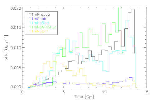
Figure 1: Star formation histories of the solar neighbourhoods associated with the five simulations; colour-coding is as noted in the inset to the panel.

3 Age-Metallicity Relations

As noted earlier, the MDF bears the imprint of a region’s star formation history (SFH), convolved with its age-metallicity relation (AMR). Having introduced the ‘solar neighbourhood’ SFHs in §2, we now present their associated AMRs in Fig 2. The time evolution of the [Fe/H] abundances are shown for each of the five simulations listed in Table 1. Colour-coding within each panel corresponds to stellar age, ranging from old (black/blue) to young (red).

To provide a representative empirical dataset against which to compare, we make use of the recent re-calibration of the Geneva-Copenhagen Survey (GCS) presented bt Holmberg et al. (2009). The base GCS provides invaluable spectral parameters for $\sim$17,000 F- and G- stars in the solar neighbourhood. Following Holmberg et al. (2007), we define a ‘cleaned’ sub-sample by eliminating (i) binary stars, (ii) stars for which the uncertainty in age is $>$25%, (iii) stars for which the uncertainty in trigonometric parallax is $>$13%, and (iv) stars for which a ‘null’ entry was provided for any of the parallax, age, metallicity, or their associated uncertainties. The AMR for this ‘cleaned’ sub-sampled of $\sim$4,000 stars is shown in the lower-right panel of Fig 2. A fifth criterion is applied for the determination of the higher-order moments of the MDF shape; specifically, following Holmberg et al. (2007) and constructing an unbiased volume-limited sub-sample from the stars lying within 40 pc of the Sun. Doing so yields a smaller sample of only $\sim$500 stars. While this does not impact on the shape characteristics of §4 or the behaviour of the AMR, for clarity, we show the AMR inferred from the aforementioned sub-sample of $\sim$4,000 stars in Fig 2.

It is worth re-emphasising that we are using the Holmberg et al. (2009) variant of the GCS solely as a useful ‘comparator’ against which to contrast our various MDF metrics / higher-order moments. It should not be interpreted as an endorsement of one solar neighbourhood MDF over another; there is a rich literature describing the various pros and cons of any number of potential selection biases within this (or any other) re-calibration of the GCS (e.g. Schoenrich & Binney, 2008; Casagrande et al., 2011) and we are not equipped to enter into that particular debate. The GCS remains the standard-bearer for MDF analysis, reflecting the nature of (fairly) volume-limited and (fairly) complete nature, making it ideal for probing the active star forming component of the thin disc; other exquisite MDFs, including those of the aforementioned (predominantly) thick disc (Schlesinger et al., 2012) and halo (Schörck et al., 2009) studies, are more suited for simulations targeting regions further from the mid-plane than we are doing here. Ideally, of course, we would like to replace the solar neighbourhood ‘comparator’ used here (the GCS) with an empirical sample more representative of star formation histories associated with massive dwarf spiral/irregulars (e.g. Skillman et al., 2003; Dolphin et al., 2003; Kirby et al., 2011), but until the statistics, completeness, and accuracy of the age and metallicity determinations for such distance dwarfs reaches that of the solar neighbourhood, we are reluctant to compare (in detail) the predictions of the simulations with those of the observations. Having said that, we will comment on, in a qualitative sense, the AMR and MDF trends seen in our simulations and how they compare with said dwarfs.

Several key points can be inferred from Fig 2. First, not surprisingly, the metallicities of the stars in the Milky Way’s solar neighbourhood (GCS) are typically a factor of $\sim$5$-$100$\times$ higher at a given age compared with the five simulations. This reflects the discussion of §2 in relation to the fact that the simulations in question are more similar to lower-luminosity disc galaxies (in terms of both mass and SFHs), rather than being Milky Way ‘clones’. The simulations are consistent with the various scaling relations to which galaxies adhere (Brook et al., 2012); as such, for their mass, their mean metallicities are a factor of $\sim$3$-$5$\times$ lower than that of the Milky Way.

More important for our purposes here, there are two additional characteristics which are readily apparent in Fig 2. First, the AMR of the solar neighbourhood is essentially non-existent, save for a trace of old, metal-poor, stars. In contrast, the corresponding regions of the simulations show extremely correlated AMRs (especially those of the fiducial simulations, 11mKroupa and 11mChab). This is partly traced to the differences in the aforementioned SFHs, although the correlation persists (admittedly with larger scatter at a given age) even in 11mNoDiff, the simulation whose SFH bears the closest resemblance to that of the Milky Way. The impact of these tightly-correlated AMRs manifest themselves significantly within the inferred MDFs, a point to which we will return in §4. Qualitatively speaking, these tightly-correlated AMRs resemble those predicted by semi-numerical galactic chemical evolution models (e.g. Chiappini et al., 2001; Fenner & Gibson, 2003; Renda et al., 2005; Mollá & Díaz, 2005).

In the bottom right panel of Fig 2, we also overplot the AMRs inferred from the colour-magnitude diagram-derived star formation histories of the dwarf irregulars Sextans A (Dolphin et al., 2003) and IC 1613 (Skillman et al., 2003); like the Milky Way, neither are meant to be one-to-one matches to the 11m series of simulations, but in some sense they do provide a useful complementary constraint, in the sense that their respective star formation histories are not dissimilar to those shown in Fig 1 (in particular, those of 11mKroupa, 11mNoMinShut, and 11mNoRad). Their associated AMRs, while lacking the statistics, completeness, and accuracy of the GCS dataset necessary to make detailed quantiative comparisons, do show evidence of possessing somewhat stronger correlations. Again, the statistics of these dwarf systems’ MDFs and AMRs make it difficult to say anything more regarding the degree of ‘agreement’ between the 11m series and that encountered in nature, but it is suggestive and certainly merits revisting once data comparable to that of the GCS becomes available for dwarf irregulars/spirals.

Second, the scatter in [Fe/H] at a given stellar age is significantly smaller (compared with that of the Milky Way) in the three simulations where the injection of thermalised massive star radiation energy to the surrounding ISM is included (i.e., 11mKroupa, 11mChab, and 11mNoMinShut). Neglecting this feedback term, within the context of these cosmological hydrodynamical disc simulations, acts to increase the scatter in [Fe/H], at a given in time, to a level comparable to that seen in Milky Way’s solar neighbourhood. Not surprisingly, the one simulation for which metal diffusion was suppressed (11mNoDiff) possesses the largest scatter in [Fe/H] at a given age, particularly at early times/low metallicities, where the neglect of diffusion is most problematic (again, a point to which we return in §4).

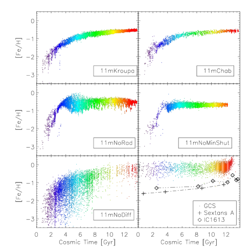
Figure 2: Age-metallicity relations (where metallicity$\equiv$[Fe/H]) in the analogous solar neighbourhoods of the five simulations employed here, in addition to the reference relationship found in the solar neighbourhood of the Milky Way and the dwarf irregulars Sextans A (Dolphin et al., 2003) and IC 1613 (Skillman et al., 2003). Colour-coding in each panel is by stellar age, ranging from black/blue (oldest) to red (youngest).

4 Metallicity Distribution Functions

Having been informed by the empirical and simulated solar neighbourhoods’ SFHs and AMRs (§2 and §3, we now present the [Fe/H] metallicity distribution functions (MDFs) for the same regions. Fig 3 shows the MDFs (black histograms) for the five simulations, the Milky Way (GCS: lower right panel) and the Local Group dwarf Fornax (also, lower right panel, from Kirby et al. (2011)). The two sub-samples of the GCS are shown; in black, the aforementioned (§3) sub-sample of $\sim$4,000 stars (matching those shown in Fig 2 – i.e., the ‘cleaned’ sub-sample, but without any distance constraint applied, labeled ‘GCS’ in the lower-right panel), and in blue, the volume-limited sample (i.e., those lying within 40 pc of the Sun, labeled ‘GCScut’). As stressed earlier, the shape characteristics of the GCS MDF are not contingent upon this latter cut; the labels ‘GCS’ and ‘GCScut’ will be employed to differentiate between the two, where relevant. Overlaid in each panel is simple ‘best-fit’ (single) Gaussian to the respective distributions (and their associated full-width at half-maximum (FWHM) values). For the Fornax dwarf, we use the full sample of 675 stars taken from Kirby et al. (2011), in order to show (perhaps) the best determined MDF for a representative local dwarf. Three caveats should be noted, in relation to the latter: (i) the sample size is 1-2 orders of magnitude smaller than the GCS, not surprisingly, considering the challenging nature of this observational work; (ii) no analogous ‘solar neighbourhood’ can be identified within this dataset (it is simply all the stars in the sample covering a range of fields in Fornax); and (iii) the uncertainty in [Fe/H] for a given individual star in Fornax is $\sim$0.5 dex, compared with the $\sim$0.1 dex associated with individual stars in the GCS. Fornax is neither better nor worse than the GCS, as a comparator, so it is useful to at least show both, as they represent the state-of-the-art, observationally-speaking.

Even before undertaking any quantitative analysis of the MDFs, it is readily apparent that the simulations (particularly, 11mKroupa, and 11mChab) possess an excess of stars to the left (i.e., to the negative side) of the peak of the MDF, relative to the right, when compared with that of the GCS and Fornax (i.e., the simulated MDFs are more negatively skewed). This ‘excess’ of lower-metallicity stars are formed in situ during the first $\sim$4 Gyrs of the simulations. The exception to this trend is 11mNoMinShut, for which the lack of significant star formation at early epochs (recall, Fig 1) and the extremely flat AMR at late times (Fig 2) conspires to present the narrow and symmetric MDF shown in Fig 3. As noted in §3, for both 11mNoRad and 11mNoDiff, the larger scatter in [Fe/H] at a given age manifests itself in the broader MDFs seen in Fig 3.

It is worth delving deeper into the source of the broader MDF seen in, for example, 11mNoRad, relative to the fiducial 11mKroupa. Here, it is at high-redshift that the radiation energy has an impact on the regulation of star formation. 11mNoRad has higher star formation at early times (Fig 1), but not at later times, primarily because it exhausts its available gas, whereas with the radiation energy star formation is regulated during that crucial period when gas accretion is at its most active; this gas remains available at later times to form stars, resulting in the MDF of 11mNoRad being broader relative to the fiducial. Ultimately, the length of time that gas spends in the disk before it forms stars shapes the MDF ‘width’ here. With radiation energy included, this gas is in the disk for a longer period of time, meaning more metal mixing occurs. Linking back to the star formation histories of Fig 1, we note that most of the gas is accreted during the first $\sim$6 Gyr, and one can see that the star formation rate shows that early peak in the case of 11mNoRad (and 11mNoDiff), but not in the cases which include radiation energy - i.e., gas that forms stars (relatively) rapidly after accretion does not mix as much, and hence the broader MDF.

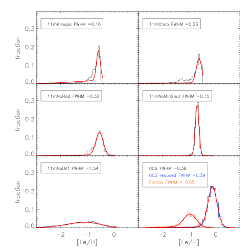
Figure 3: The [Fe/H] metallicity distribution functions in the solar neighourhoods of the five simulations employed here. The bottom-right panel shows the MDF of the Milky Way’s solar neighbourhood, based upon two sub-samples of stars selected from Holmberg et al. (2009), as well as that for Local Group dwarf Fornax, from Kirby et al. (2011) (see text for details). In each panel, the overlaid curve is the best-fit single component Gaussian to the aforementioned MDF; the associated FWHM of said Gaussian is listed in the inset to each panel.

Simulation/Dataset	Skewness	Kurtosis	IQR	IDR	ICR	ITPR
11mKroupa	$-$1.84($-$1.21)	3.83(2.59)	0.30(0.54)	0.67(1.13)	1.59(2.72)	2.49(4.34)
11mChab	$-$1.56($-$1.15)	2.43(2.37)	0.41(0.60)	0.85(1.28)	1.71(2.96)	2.38(5.04)
11mNoRad	$-$1.13($-$0.93)	2.45(1.88)	0.26(0.47)	0.52(0.92)	1.44(2.07)	2.39(3.73)
11mNoMinShut	$+$0.47($-$0.29)	0.94(0.57)	0.13(0.48)	0.26(0.93)	0.69(1.79)	1.97(3.26)
11mNoDiff	$-$0.91($-$1.29)	0.91(2.32)	0.96(1.25)	1.85(2.44)	3.49(5.18)	5.06(8.03)
GCS	$-$0.61	2.04	0.23	0.48	1.26	2.63
GCScut	$-$0.37	0.78	0.24	0.45	0.94	1.43
Fornax	($-$1.33)	(3.58)	(0.38)	(2.25)	(2.75)	(2.85)

Table 2: Primary MDF shape characteristics for the solar neighbourhoods of the five simulations described here, the two sub-samples based upon the Holmberg et al. (2009) GCS empirical dataset are as described in the text and data for the Fornax dwarf galaxy taken from Kirby et al. (2011). After Fenner & Gibson (2003), the simulated MDFs were convolved with either a 0.1 dex Gaussian (left-most entry within each column) or a 0.5 dex Gaussian (right-most / bracketed entry within each column), to mimic the typical uncertainties associated with the [Fe/H] determinations in nature (the GCS in the case of the former, and Fornax in the case of the latter). Column (1): the name of the simulation or empirical dataset; Column (2): the skewness of the MDF (5$\sigma$ clipping of outliers was imposed, to minimise their impact on the determination); Column (3): the kurtosis of the MDF, again with the adoption of 5$\sigma$ clipping; Columns (4) $-$ (7): the interquartile (IQR), interdecile (IDR), intercentile (ICR), and inter-tenth-percentile (ITPR) for each MDF.

We next undertook a quantitative analysis of the MDFs shown in Fig 3, including a determination of the skewness, kurtosis, and widths at a range of inter-percentiles of the distributions. These determinations are listed in Table 2. As both skewness and kurtosis are highly sensitive to the presence of outliers, we imposed a fairly standard 5$\sigma$ clipping to the distributions. To mimic the observational uncertainties associated with the determination of individual stellar [Fe/H] abundances, after Fenner & Gibson (2003), the ‘theoretical’ MDFs shown in Fig 3 were convolved first with either a 0.1 dex Gaussian (to mimic the GCS uncertainties - Holmberg et al. 2009) or a 0.5 dex Gaussian (to mimic the uncertainties with the Fornax data - Kirby et al. 2011). In Table 2, each column has two numbers; the first is the relevant metric, as measured on the MDF convolved with a 0.1 dex Gaussian, while the second (in brackets) is that measured on the MDF convolved with a 0.5 dex Gaussian. As the simulated MDFs are typically much broader than the GCS uncertainties, the impact of the 0.1 dex smoothing is minimal.

As inferred from the above qualitative discussions of the MDF and the AMR (§3), MDFs of the simulated solar neighbourhoods are all (save for 11mNoMinShut, whose exceedingly flat AMR results in the elimination of essentially all tails, positive or negative of the MDF’s peak) more negatively skewed than that of the Milky Way’s solar neighbourhood (from both the volume-limited GCScut sample of stars, and the unrestricted GCS sample) and the sample from Fornax. It must be emphasised though that the typical 0.5 dex uncertainty associated with the determination of [Fe/H] for individual stars in Fornax means that broadening the simulated MDFs, with their typical dispersions of $\sim$0.1 dex, by 0.5 dex, ‘washes out’ much of our ability to compare and contrast the higher-order MDF metrics, and hence the analysis which follows emphasises the differences between the simulated MDFs and that of the GCS. The ‘tail’ of stars to the negative side of the peak should not be associated immediately with the traditional ‘G-dwarf problem’, since these fully cosmological simulations relax the ‘closed-box’ framework which is the hallmark of this problem. Instead, as noted earlier, it is the tightly-correlated AMRs which are driving the large negative skewness values; these AMRs do not resemble that of the Milky Way’s solar neighbourhood. The different SFHs are certainly part of the difference, but as noted earlier, both the fiducial 11mChab and 11mNoDiff show SFHs not dissimilar to the exponentially-declining one of the Milky Way, and the coordinated AMRs remain responsible for the larger negative skewness in both cases. An analysis of the kurtosis values for each distribution are consistent with this picture. Specifically, the simulations’ kurtosis values are all larger than those of GCScut, and as noted in §2, large kurtosis values are driven in part by the presence of a ‘peaky’ MDF, but more importantly, the impact of extended, ‘heavy’, tails. These tails (postive or negative) are driven by the coordinated AMRs and are reflected in the generally large values of kurtosis relative to the Milky Way’s distribution.

Alongside the skewness and kurtosis determinations, we present four measures of the shape of the MDF, through its dispersion, or width, at different amplitudes. This is done via the width of the inter-quartile range (IQR), inter-decile range (IDR), inter-centile range (ICR), and the inter-tenth-percentile range (ITPR).

The metrics associated with these width measures require some comment in relation to the information provided by Fig 3. Specifically, the best-fit single Gaussian fits overlaid in each panel show that grossly speaking, the Milky Way’s and Fornax’s MDF are broader than those associated with the simulations. At first glance, the IQR, ITR, etc, measures listed in Table 2 appear counter to this result (which are all, essentially, larger than the values found for GCScut, for example). It is important to remember though that, much like the case for skewness and kurtosis, these measures of the breadth of the MDF are sensitive to the impact of outliers in the tails of the distribution.

It is particularly useful to note the quantitative impact of the role of metal diffusion in setting the width of the MDF in tails of the distribution. For example, in the solar neighbourhood of the Milky Way, the range in metallicity between the bottom and top 0.1% of the stars is $\sim$2 dex. For our simulation in which metal diffusion was neglected (11mNoDiff), the corresponding width is $\sim$5 dex – i.e., a factor of $\sim$1000$\times$ greater than the other simulations with diffusion and that encountered in the Milky Way, similar to what we found for other low diffusion runs (Pilkington et al., 2012).

After Casagrande et al. (2011), we show in Fig 4 the MDF for the solar neighbourhood of one of our fiducial simulations (11mKroupa), but now binned more finely in metallicity and colour-coded by age. Here, young stars correspond to those formed in the last 1 Gyr at redshift $z$=0; intermediate-age stars are those with ages between 5 and 7 Gyrs; old corresponds to stars with ages greater than 9 Gyrs. Using the GCS, Casagrande et al. (2011) conclude that the younger stars have a narrower MDF that the older stars, consistent with our results (and to be expected, given its AMR). Casagrande et al. (2011) also found though that the locations of the peaks associated with these old and young stars were at the same metallicity, which is not consistent with our simulations. Again, this is to be expected given the tightly-correlated AMRs of the simulations, relative to that of the Milky Way.

While it may be the case that we are not capturing all of the relevant stellar migration physics within these simulations (e.g., bars, spiral arms, resonances, etc.), there is radial migration occurring. That said, the radial gradients are shallow for these fiducial dwarfs ($-$0.01$-$0.02 dex/kpc, recalling Table 1) and, as such, over the few kpcs of ‘disc’ associated with each simulated dwarf, systematic migration of metal-rich inner-disc stars outwards (and vice versa) has little impact on the position of the MDF ‘sub-structure’ (in which the young, intermediate, and old ‘peaks’ are offset by $\sim$0.3$-$0.5 dex from one another). Again, this is entirely consistent with the expected behaviour, based upon the AMR Fig 2.

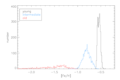
Figure 4: The [Fe/H] MDF in the ‘solar neighbourhood’ of 11mKroupa, split into three age intervals: young (black) defined as any star particle in the solar neighbourhood at redshift $z$=0 with an age less than 1 Gyr; intermediate (blue) defined as any star with an age between 5 and 7 Gyr; old (red) defined as any star with an age greater than 9 Gyr.

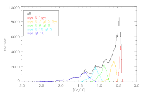
Figure 5: The [Fe/H] MDF of the ‘bulge’ of 11mKroupa; here, the bulge is simply defined as those stars located within 2 kpc of the galactic centre at $z$=0. Alongside the full MDF (black line), sub-components based upon the age intervales noted in the inset are overdrawn.

The central regions of our simulations show similar characteristics to those seen in the simulated solar neighbourhoods. Specifically, the [Fe/H] MDF of the ‘bulge’ (inner 2 kpc) shows a peak near [Fe/H]$\sim$$-$0.5, with a number of sub-components at lower metallicity which correspond to progressively older and metal-poor populations (see Fig 5). In spirit, such behaviour has been seen in the MDF of the bulge of the Milky Way, where Bensby et al. (2011) finds two populations, also separated comparably in age and metallicity, to which they associate seaprate formation scenarios. Similarly, Hill et al. (2011) finds bulge sub-components within the MDF which they also separate into separate age, metallicity, and kinematic sub-structures, concluding the metal-poor component can be associated with an old spheroid, and the more metal-rich component can be associated with a longer timescale event (perhaps the evolution of the bar / psudeo-bulge). In our simulations, we see systematic trends in age and kinematics for each metallicity sub-component of Fig 5, in the sense of the more metal-poor components being older and progressively less rotationally-supported, in exactly the manner one might predict from the AMR (§3). It should be emphasised though that within the simulations, the behaviour of these age, metallicity, and kinematic ‘sub-structure’ in the bulge MDF is continuous, rather than showing any discrete transition from rotational support to anisotropic velocity support.

Finally, we now examine in slightly more detail the behaviour of the extreme metal-poor tails of the simulated MDFs (see Figs 6 and 7). In Fig 6, we show all stars beyond the inner 3 kpc (and within 10 kpc), in order to minimise the effect of the ‘spheroid’ stars in the analysis. We experimented, as before, with the impact of using a full kinematic decomposition between disc and spheroid stars, but again, for these dwarfs, the spatial cut alone is indistinguishable from the decomposed galaxy. In Fig 7, we only show those star particles lying within the previously defined ‘solar neighbourhoods’ of each simulation.

One additional curve is included in both figures (labeled 109CH), that of the disc generated with the adaptive mesh refinement code Ramses and described by Sánchez-Blázquez et al. (2009), in which diffusion is handled ‘naturally’. As noted previously, each of the 11m series of simulations employ the Shen et al. (2010) metal diffusion framework with a diffusion coefficient C=0.05, except for (obviously) 11mNoDiffwhich assumes C=0.0.

Each of the cumulative MDFs (Figs 6 and 7) are normalised. In both cases, the normalisation occurs at the [Fe/H] corresponding to the metallicity of the lowest 1% of the stars (in terms of [Fe/H]). For plotting purposes, these are then aligned arbitrarily at [Fe/H]$\equiv$+0.0, to show the relative distributions of extremely low-metallicity stars within each simulation and the empirical datasets. One could take a different approach and, say, normalise at (i) the same metallicity, (ii) the same amplitude, or (iii) the same number of stars. For example, in our analysis of the Governato et al. (2010) bulgeless dwarf galaxy simulations (Pilkington et al., 2012), we adopted (i), normalising all MDFs at [Fe/H]=$-$2.3. This was similar in spirit to Schörck et al. (2009), who fixed the normalisations of the Milky Way halo and Local Group dwarf spheroidal MDFs to be unity at the metallicity corresponding to the lowest (in terms of [Fe/H]) $\sim$100 stars in each. For distributions which peak at (potentially) very different metallicities, such normalisations can result in significant outliers which are not necessarily driven by any MDF ‘tail’. For our work here, while small quantitative differences exist depending upon the adopted normalisation, the qualitative results are robust regardless of the choice.

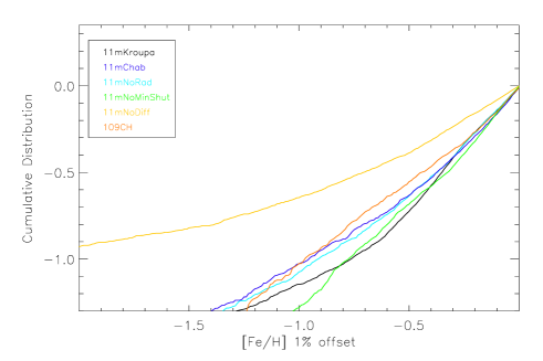
Figure 6: The cumulative MDFs of the five 11m simulations: 11mKroupa (black), 11mNoRad (cyan), 11mChab (blue), 11mNoMinShut (green), and 11mNoDiff (gold), in addition to that of 109CH (orange: Sánchez-Blázquez et al. (2009)). For these six simulations, all stars lying within 3 and 10 kpc of their respective galactic centres are included in the analysis. The normalisation in each case is at the metallicity corresponding to that of the lowest 1% (in terms of [Fe/H]) of the stars in each case.

What is immediately clear from even a cursory examination of Fig 6 is that the relative distribution of extremely metal-poor stars within all the simulations in which metal diffusion acts - i.e., all but 11mNoDiff - are consistent with each other. This reflects graphically what we have commented upon earlier in relation to the tabulated ICR and ITPR values for the various MDFs (Table 2). Specifically, the lack of metal diffusion within 11mNoDiff drives its discrepant ICR and ITPR values (Table 2), and its outlier status in Fig 6. When compared with Fig 5 of Pilkington et al. (2012), one can see that the overly ‘heavy’ metal-poor tail to the MDF of 11mNoDiff matches that encountered in, for example, the low metal-diffusion simulations of Governato et al. (2010). One fairly robust conclusion that can be drawn from Fig 6 is that the relative distribution of extremely metal-poor stars is robust against the choice of feedback scheme; instead, diffusion plays a more important role in shaping this distribution.

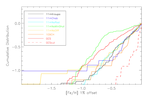
Figure 7: The cumulative MDFs of the analogous solar neighbourhoods associated the five 11m simulations: 11mKroupa (black), 11mNoRad (purple), 11mChab (blue), 11mNoMinShut (green), and 11mNoDiff (gold), in addition to that of 109CH (orange: Sánchez-Blázquez et al. (2009)). For these six simulations, the solar neighbourhood is defined spatially to include stars lying between 3 and 3.5 disc scalelengths from their respective galactic centres, and within 0.5 kpc of the mid-plane. The GCS and GCScut sub-samples described in §2 are shown in red. The normalisation for each curve is as described for Fig 6.

In some sense, the better ‘statistics’ afforded by Fig 6 provides a ‘cleaner’ picture than that seen when restricting the analysis to just the ‘solar neighbourhoods’. For completeness though, in Fig 7 we also show the cumulative MDFs of the metal-poor tails for each dataset, normalised as in Fig 6. We should emphasise though that the small number of star particles in the ‘bottom’ 1% (in terms of metallicity) of the 11mNoDiff, 11mChab, and GCScut samples ($\sim$30 in each) make any interpretation susceptible to small-number statistics (and stochastic point-to-point ‘fluctuations’ which are ‘averaged’ over when employed the full disc, as in Fig 6).

5 Summary

Employing a suite of five simulations of an M33-scale late-type disc galaxy, each with the same assembly history, but with different prescriptions for stellar and supernovae feedback, initial mass functions, metal diffusion, and supernova remnant cooling ‘shut-off’ period, we have analysed the resulting chemistry of the stellar populations, with a particular focus on the metallicity distribution functions and the characteristics of the extreme metal-poor tail of said distributions.

In the context of the distribution of metals (in the sense of the higher-order moments of the resultings MDFs) within these discs, the impact of feedback and the IMF is more subtle than that of, for example, metal diffusion. Employing a Chabrier (2003) IMF, rather than the Kroupa et al. (1993) form adopted in our earlier work, does impact significantly on the resulting star formation history (and associated, reduced, stellar mass fraction, resulting in remarakably close adherence to a wade range of empirical scaling relations - Brook et al. (2011c)).

The star formation histories of the ‘solar’ neighbourhoods associated with each simulation show exceedingly tight age-metallicity relations. In shape, these relations are akin to those predicted by classical galactic chemical evolution models (e.g. Chiappini et al., 2001; Fenner & Gibson, 2003), but bear somewhat less resemblance to that seen, for example, in the Milky Way’s solar neighbourhood (Holmberg et al., 2009). These correlated age-metallicity relations result inexorably in (negatively) skewed MDFs with large kurtosis values, when compared with the Milky Way. Star formation histories of dwarf irregulars, which qualitatively speaking are a better match to those of the 11m series of simulations presented here, suggest though that somewhat steeper age-metallicity relations might eventuate in nature in these environments (e.g. Dolphin et al., 2003; Skillman et al., 2003). MDFs and AMRs of a comparable quality to that of the GCS (Holmberg et al., 2009) will be required to subtantively progress the field.

An excess ‘tail’ of extremely metal-poor stars (amongst the bottom 0.1$-$1% of the most metal-poor stars) – $\sim$2$-$3 dex below the peak of the MDF – exists in all of the simulations, as reflected in their inter-centile (ICR) and inter-tenth-of-a-percentile (ITPR) region measures. This tail is particularly problematic in simulations without metal diffusion (11mNoDiff) and those for which the diffusion coefficient was set relatively low (e.g. Governato et al., 2010; Pilkington et al., 2012). As demonstrated, the ICR and ITPR, in the absence of metal diffusion, can be $\sim$30$-$3000$\times$ larger than that encountered in the Milky Way.

We end with a re-statement of our initial caveat. The simulations presented here (particularly the fiducials, 11mKroupa and 11mChab) have been shown to be remarkably consistent with a wide range of scaling relations (Brook et al., 2012). That said, their star formation histories are more akin to those of NGC 6822, Sextans A, WLM, and to some extent, the LMC (at least in the case of 11mChab) – i.e., these systems are not ‘clones’ of the Milky Way. We have used the wonderful Geneva-Copenehagen Survey’s wealth of data to generate empirical age-metallicity relations and metallicity distribution functions against which to compare, but exact one-to-one matches are not to be expected. That said, they do provide useful, hopefully generic, relations against which to compare. In the future, we hope to extend our analysis to equally comprehensive datasets for the LMC, making use of, for example, the data provided by the Vista Magellanic Cloud Survey (Cioni et al., 2011).

References

- Abadi et al. (2003) Abadi M. G., Navarro J. F., Steinmetz M., Eke V. R., 2003, \apj, 597, 21
- Asplund et al. (2009) Asplund M., Grevesse N., Sauval A. J., Scott P., 2009, \araa, 47, 481
- Bensby et al. (2011) Bensby T., Adén D., et al. 2011, \aap, 533, A134
- Brook et al. (2012) Brook C. B., Stinson G., Gibson B. K., Roškar R., Wadsley J., Quinn T., 2012, \mnras, 419, 771
- Brook et al. (2012) Brook C. B., Stinson G., Gibson B. K., Wadsley J., Quinn T., 2012, ArXiv e-prints
- Caimmi (2008) Caimmi R., 2008, \na, 13, 314
- Calura et al. (2012) Calura F., Gibson B. K., Michel-Dansac L., Stinson G. S., Pilkington K., House E. L., Brook C. B., Few C. G., Bailin J., Couchman H. M. P., Wadsley J., . 2012, ArXiv e-prints
- Carrera et al. (2008) Carrera R., Gallart C., Aparicio A., Costa E., Méndez R. A., Noël N. E. D., 2008, \aj, 136, 1039
- Casagrande et al. (2011) Casagrande L., Schönrich R., Asplund M., Cassisi S., Ramírez I., Meléndez J., Bensby T., Feltzing S., 2011, \aap, 530, A138+
- Chabrier (2003) Chabrier G., 2003, \pasp, 115, 763
- Chiappini et al. (2001) Chiappini C., Matteucci F., Romano D., 2001, \apj, 554, 1044
- Cioni et al. (2011) Cioni M.-R. L., Clementini G., et al. 2011, \aap, 527, A116
- Dolphin et al. (2003) Dolphin A. E., Saha A., Skillman E. D., Dohm-Palmer R. C., Tolstoy E., Cole A. A., Gallagher J. S., Hoessel J. G., Mateo M., 2003, \aj, 126, 187
- Dolphin et al. (2005) Dolphin A. E., Weisz D. R., Skillman E. D., Holtzman J. A., 2005, ArXiv Astrophysics e-prints
- Fenner & Gibson (2003) Fenner Y., Gibson B. K., 2003, \pasa, 20, 189
- Gibson (1994) Gibson B. K., 1994, JRASC, 88, 383
- Gibson et al. (2001) Gibson B. K., Giroux M. L., Penton S. V., Stocke J. T., Shull J. M., Tumlinson J., 2001, \aj, 122, 3280
- Governato et al. (2010) Governato F., Brook C., Mayer L., Brooks A., Rhee G., Wadsley J., Jonsson P., Willman B., Stinson G., Quinn T., Madau P., 2010, \nat, 463, 203
- Haardt & Madau (1996) Haardt F., Madau P., 1996, \apj, 461, 20
- Hartwick (1976) Hartwick F. D. A., 1976, \apj, 209, 418
- Haywood (2001) Haywood M., 2001, \mnras, 325, 1365
- Hill et al. (2011) Hill V., Lecureur A., Gómez A., Zoccali M., Schultheis M., Babusiaux C., Royer F., Barbuy B., Arenou F., Minniti D., Ortolani S., 2011, \aap, 534, A80
- Holmberg et al. (2007) Holmberg J., Nordström B., Andersen J., 2007, \aap, 475, 519
- Holmberg et al. (2009) Holmberg J., Nordström B., Andersen J., 2009, \aap, 501, 941
- Holtzman et al. (1999) Holtzman J. A., Gallagher III J. S., Cole A. A., Mould J. R., Grillmair C. J., Ballester G. E., Burrows C. J., Clarke J. T., Crisp D., Evans R. W., Griffiths R. E., Hester J. J., Hoessel J. G., Scowen P. A., Stapelfeldt K. R., Trauger J. T., Watson A. M., 1999, \aj, 118, 2262
- Hopkins et al. (2011) Hopkins P. F., Quataert E., Murray N., 2011, \mnras, 417, 950
- Kannan et al. (2012) Kannan R., Macciò A. V., Pasquali A., Moster B. P., Walter F., 2012, \apj, 746, 10
- Kirby et al. (2011) Kirby E. N., Lanfranchi G. A., Simon J. D., Cohen J. G., Guhathakurta P., 2011, \apj, 727, 78
- Kobayashi & Nakasato (2011) Kobayashi C., Nakasato N., 2011, \apj, 729, 16
- Kotoneva et al. (2002) Kotoneva E., Flynn C., Chiappini C., Matteucci F., 2002, \mnras, 336, 879
- Kroupa et al. (1993) Kroupa P., Tout C. A., Gilmore G., 1993, \mnras, 262, 545
- Macciò et al. (2012) Macciò A. V., Stinson G., Brook C. B., Wadsley J., Couchman H. M. P., Shen S., Gibson B. K., Quinn T., 2012, \apjl, 744, L9
- McClure-Griffiths et al. (2006) McClure-Griffiths N. M., Ford A., Pisano D. J., Gibson B. K., Staveley-Smith L., Calabretta M. R., Dedes L., Kalberla P. M. W., 2006, \apj, 638, 196
- Mollá & Díaz (2005) Mollá M., Díaz A. I., 2005, \mnras, 358, 521
- Nordström et al. (2004) Nordström B., Mayor M., Andersen J., Holmberg J., Pont F., Jørgensen B. R., Olsen E. H., Udry S., Mowlavi N., 2004, \aap, 418, 989
- Pagel & Patchett (1975) Pagel B. E. J., Patchett B. E., 1975, \mnras, 172, 13
- Pilkington et al. (2012) Pilkington K., Few C. G., Gibson B. K., Calura F., Michel-Dansac L., Thacker R. J., Mollá M., Matteucci F., Rahimi A., Kawata D., Kobayashi C., Brook C. B., Stinson G. S., Couchman H. M. P., Bailin J., Wadsley J., 2012, \aap, 540, A56
- Pilkington et al. (2012) Pilkington K., Gibson B. K., Calura F., Stinson G. S., Brook C. B., Brooks A., 2012, in JENAM 2010, Joint European and National Astronomy Meeting The Chemical and Dynamical Evolution of Isolated Dwarf Galaxies
- Raiteri et al. (1996) Raiteri C. M., Villata M., Navarro J. F., 1996, \memsai, 67, 817
- Renda et al. (2005) Renda A., Kawata D., Fenner Y., Gibson B. K., 2005, \mnras, 356, 1071
- Robertson & Kravtsov (2008) Robertson B. E., Kravtsov A. V., 2008, \apj, 680, 1083
- Roškar et al. (2008) Roškar R., Debattista V. P., Quinn T. R., Stinson G. S., Wadsley J., 2008, \apjl, 684, L79
- Sánchez-Blázquez et al. (2009) Sánchez-Blázquez P., Courty S., Gibson B. K., Brook C. B., 2009, \mnras, 398, 591
- Schlesinger et al. (2012) Schlesinger K. J., Johnson J. A., et al. 2012, ArXiv e-prints
- Schoenrich & Binney (2008) Schoenrich R., Binney J., 2008, ArXiv e-prints
- Schörck et al. (2009) Schörck T., Christlieb N., Cohen J. G., Beers T. C., Shectman S., Thompson I., 2009, \aap, 507, 817
- Shen et al. (2010) Shen S., Wadsley J., Stinson G., 2010, \mnras, pp 1043–+
- Skillman et al. (2003) Skillman E. D., Tolstoy E., Cole A. A., Dolphin A. E., Saha A., Gallagher J. S., Dohm-Palmer R. C., Mateo M., 2003, \apj, 596, 253
- Sommer-Larsen & Fynbo (2008) Sommer-Larsen J., Fynbo J. P. U., 2008, \mnras, 385, 3
- Springel et al. (2008) Springel V., Wang J., Vogelsberger M., Ludlow A., Jenkins A., Helmi A., Navarro J. F., Frenk C. S., White S. D. M., 2008, \mnras, 391, 1685
- Stinson et al. (2012) Stinson G., Brook C., Prochaska J. X., Hennawi J., Pontzen A., Shen S., Wadsley J., Couchman H., Quinn T., Macciò A. V., Gibson B. K., 2012, ArXiv e-prints
- Stinson et al. (2006) Stinson G., Seth A., Katz N., Wadsley J., Governato F., Quinn T., 2006, \mnras, 373, 1074
- Stinson et al. (2010) Stinson G. S., Bailin J., Couchman H., Wadsley J., Shen S., Nickerson S., Brook C., Quinn T., 2010, \mnras, 408, 812
- Tinsley (1980) Tinsley B. M., 1980, \fcp, 5, 287
- Tissera et al. (2011) Tissera P. B., White S. D. M., Scannapieco C., 2011, ArXiv e-prints
- Tumlinson et al. (2011) Tumlinson J., Thom C., et al. 2011, Science, 334, 948
- van den Hoek & Groenewegen (1997) van den Hoek L. B., Groenewegen M. A. T., 1997, \aaps, 123, 305
- Vera-Ciro et al. (2012) Vera-Ciro C. A., Helmi A., Starkenburg E., Breddels M. A., 2012, ArXiv e-prints
- Wadsley et al. (2004) Wadsley J. W., Stadel J., Quinn T., 2004, New Astronomy, 9, 137
- Wiersma et al. (2011) Wiersma R. P. C., Schaye J., Theuns T., 2011, ArXiv e-prints
- Woosley & Weaver (1995) Woosley S. E., Weaver T. A., 1995, \apjs, 101, 181