Testing the Standard Model and searching for New Physics with $B_{d}\to\pi\pi$ and $B_{s}\to KK$ decays

Abstract

We propose to perform a combined analysis of $B\to\pi\pi$ and $B_{s}\to K^{+}K^{-}$ modes, in the framework of a global CKM fit. The method optimizes the constraining power of these decays and allows to derive constraints on NP contributions to penguin amplitudes or on the $B_{s}$ mixing phase. We illustrate these capabilities with a simplified analysis using the recent measurements by the LHCb Collaboration, neglecting correlations with other SM observables.

CP violation in $B_{d,s}$ decays plays a fundamental role in testing the consistency of the Cabibbo-Kobayashi-Maskawa (CKM) paradigm in the Standard Model (SM) and in probing virtual effects of heavy new particles. With the advent of the B-factories, the Gronau-London (GL) isospin analysis of $B_{d}\to\pi\pi$ decays Gronau and London (1990) has been a precious source of information on the phase of the CKM matrix. Although the method allows a full determination of the weak phase and of the relevant hadronic parameters, it suffers from discrete ambiguities that limit its constraining power. It is however possible to reduce the impact of discrete ambiguities by adding information on hadronic parameters Charles (1999); Bona et al. (2007). In particular, as noted in refs. Fleischer (1999, 2007); Fleischer and Knegjens (2011), the hadronic parameters entering the $B_{d}\to\pi^{+}\pi^{-}$ and the $B_{s}\to K^{+}K^{-}$ decays are connected by U-spin, so that the experimental knowledge of $B_{s}\to K^{+}K^{-}$ can definitely improve the extraction of the CKM phase with the GL analysis. Indeed, in ref. Bona et al. (2007), the measurement of $\mathrm{BR}(B_{s}\to K^{+}K^{-})$ was used to obtain an upper bound on one of the hadronic parameters.

After the pioneering studies performed at the TeVatron, very recently LHCb opened up the road to CP violation in $B_{s}\to KK$ decays LHC (2012a). The present experimental information is summarized in Table 1. At present, one has all the necessary information to use the U-spin strategy proposed by Fleischer (F) in refs. Fleischer (1999, 2007) to extract the CKM phase from a combined analysis of $B_{d}\to\pi^{+}\pi^{-}$ and the $B_{s}\to K^{+}K^{-}$ decays. However, as we will show explicitly below, this strategy alone suffers from a sizable dependence on the breaking of U-spin symmetry Beneke (2003).

Furthermore, in the $B_{s}$ system the measurement of any time-dependent CP asymmetry cannot be directly translated into a measurement of the angle $\beta_{s}=\mathrm{arg}\,\left(-\frac{V_{tb}^{*}V_{ts}}{V_{cb}^{*}V_{cs}}\right)$, even in the case of the so-called “gold-plated” $b\to c\bar{c}s$ decays. This is due to the fact that the angle $\beta_{s}$ is small and correlated to the subdominant amplitude in $b\to c\bar{c}s$ decays. Thus, measuring $\beta_{s}$ requires the determination of the subdominant decay amplitude. This is evident by noting that using CKM unitarity the $b\to s$ decay amplitude can be written as

$$A=V_{ub}V_{us}^{*}T+V_{cb}V_{cs}^{*}P\quad\mathrm{or}\quad A=V_{ub}V_{us}^{*}(T-P)+V_{tb}V_{ts}^{*}(-P).$$ (1)

Naively dropping the doubly Cabibbo-suppressed term proportional to $V_{ub}V_{us}^{*}$ would lead to the conclusion that the CP asymmetry measures $2\beta_{s}$ with the first choice or that the CP asymmetry should vanish in the second choice. Clearly, a full treatment of the decay amplitude, taking into account correlations between the various CKM terms, is necessary to give a meaningful interpretation to the CP asymmetry. This is at variance with the $B_{d}$ case, where the angle $\beta$ is large and thus the time-dependent CP asymmetry in $b\to c\bar{c}s$ decays gives sin$2\beta$ with a good accuracy. In this respect, the combined analysis of the GL modes and $B_{s}\to K^{+}K^{-}$ is optimal, since one has full knowledge of the U-spin related control channel $B_{d}\to\pi^{+}\pi^{-}$, similarly to the case of $B_{s}\to K^{(*)0}\bar{K}^{(*)0}$ and $B_{d}\to K^{(*)0}\bar{K}^{(*)0}$ proposed in ref. Ciuchini et al. (2008). Conversely, the “gold-plated” $B_{s}\to J/\psi\phi$ decay has no U-spin related control channel, making the extraction of $\beta_{s}$ problematic Faller et al. (2009b).

Channel	BR $\times 10^{6}$	$\mathcal{S}(\%)$	$\mathcal{A}_{\mathrm{CP}}(=-\mathcal{C})(\%)$	corr.	ref.
$B_{d}\to\pi^{+}\pi^{-}$	$5.11\pm 0.22$	$-65\pm 7$	$38\pm 6$	$0.08$	Aubert et al. (2008); Ishino et al. (2007); Aubert et al. (2007a); Chang (2011); Bornheim et al. (2003); Aaltonen et al. (2011)
$B_{d}\to\pi^{+}\pi^{-}$	–	$-56\pm 17\pm 3$	$11\pm 21\pm 3$	$-0.34$	LHC (2012a)
$B_{d}\to\pi^{0}\pi^{0}$	$1.91\pm 0.23$	–	$43\pm 24$	–	Aubert et al. (2008); Abe et al. (2005); Bornheim et al. (2003)
$B^{+}\to\pi^{+}\pi^{0}$	$5.48\pm 0.35$	–	$2.6\pm 3.9$	–	Aubert et al. (2007b); Chang (2011); Bornheim et al. (2003)
$B_{s}\to K^{+}K^{-}$	$25.4\pm 3.7$	$17\pm 18\pm 5$	$2\pm 18\pm 4$	$-0.1$	Peng et al. (2010); Aaltonen et al. (2011); LHC (2012a)

Table 1: Experimental data used in the analysis. The correlation column refers to the $\mathcal{S}$ and $\mathcal{A}_{\mathrm{CP}}$ measurements. Except from the results in ref. LHC (2012a), all other measurements have been averaged by HFAG *[][andonlineupdateathttp://www.slac.stanford.edu/xorg/hfag]HFAG. The CP asymmetry of $B^{+}\to\pi^{+}\pi^{0}$ has been reported for completeness, although it has not been used in the analysis.

We propose to perform a combined analysis of the GL modes plus $B_{s}\to K^{+}K^{-}$, including the time-dependent CP asymmetries, to obtain an optimal determination of the CKM phase within the SM. We show that this combined strategy has a mild dependence on the magnitude of U-spin breaking, allowing for a solid estimate of the theory error.

Beyond the SM, NP can affect both the $B_{d,s}-\bar{B}_{d,s}$ amplitudes and the $b\to d,s$ penguin amplitudes. Taking the phase of the mixing amplitudes from other measurements, for example from $b\to c\bar{c}s$ decays, one can obtain a constraint on NP in $b\to s$ penguins. Alternatively, assuming no NP in the penguin amplitudes, one can obtain a constraint on NP in mixing.

In this letter, we illustrate the points above in a simplified framework, neglecting SM correlations with other observables and using as input values sin$2\beta=0.679\pm 0.024$ Asner et al. (2010) and $2\beta_{s}=(0\pm 5)^{\circ}$ LHC (2012b), obtained from $b\to c\bar{c}s$ decays. Clearly, the optimal strategy will be to include the combined analysis of the GL and F modes in a global fit of the CKM matrix plus possible NP contributions.

The GL and F analyses were formulated with different parameterizations of the decay amplitudes. In order to use the constraints in a global fit, one should write the decay amplitudes with the full dependence on CKM matrix elements, but for the present analysis we can choose the F one and write the amplitudes as follows:

$$\begin{array}[]{ll}A(B_{d}\to\pi^{+}\pi^{-})=C(e^{i\gamma}-de^{i\theta})\,,&A(\bar{B}_{d}\to\pi^{+}\pi^{-})=C(e^{-i\gamma}-de^{i\theta})\,,\\ A(B_{d}\to\pi^{0}\pi^{0})=\frac{C}{\sqrt{2}}(Te^{i\theta_{T}}e^{i\gamma}+de^{i\theta})\,,&A(\bar{B}_{d}\to\pi^{0}\pi^{0})=\frac{C}{\sqrt{2}}(Te^{i\theta_{T}}e^{-i\gamma}+de^{i\theta})\,,\\ A(B^{+}\to\pi^{+}\pi^{0})=\frac{A(B_{d}\to\pi^{+}\pi^{-})}{\sqrt{2}}+A(B_{d}\to\pi^{0}\pi^{0})\,,&A(B^{-}\to\pi^{-}\pi^{0})=\frac{A(\bar{B}_{d}\to\pi^{+}\pi^{-})}{\sqrt{2}}+A(\bar{B}_{d}\to\pi^{0}\pi^{0})\,,\\ A(B_{s}\to K^{+}K^{-})=C^{\prime}\frac{\lambda}{1-\lambda^{2}/2}(e^{i\gamma}+\frac{1-\lambda^{2}}{\lambda^{2}}d^{\prime}e^{i\theta^{\prime}})\,,&A(\bar{B}_{s}\to K^{+}K^{-})=C^{\prime}\frac{\lambda}{1-\lambda^{2}/2}(e^{-i\gamma}+\frac{1-\lambda^{2}}{\lambda^{2}}d^{\prime}e^{i\theta^{\prime}})\,,\end{array}$$ (2)

where the magnitude of $V_{ub}V_{ud}$ has been reabsorbed in $C$, the magnitude of $V_{cb}V_{cd}/(V_{ub}V_{ud})$ has been reabsorbed in $d$ and $\lambda=0.2252$. In the exact U-spin limit, one has $C=C^{\prime}$, $d=d^{\prime}$ and $\theta=\theta^{\prime}$. We have neglected isospin breaking in $B_{d}\to\pi\pi$, since its impact on the extraction of the weak phase is at the level of $1^{\circ}$ Gronau et al. (1999); Zupan (2007); Gardner (2005); Botella et al. (2006). The physical observables entering the analysis are:

$$BR(B\to MM)=F(B)\frac{|A(B\to MM)|^{2}+|A(\bar{B}\to MM)|^{2}}{2}\,,$$ (3)

$$\mathcal{A}_{\mathrm{CP}}=-\mathcal{C}=\frac{|A(\bar{B}\to MM)|^{2}-|A(B\to MM)|^{2}}{|A(\bar{B}\to MM)|^{2}+|A(B\to MM)|^{2}}\,,\qquad\mathcal{S}=\frac{2\mathrm{Im}\left(e^{-i\phi_{M}(B)}\frac{A(\bar{B}\to MM)}{A(B\to MM)}\right)}{1+\left|\frac{A(\bar{B}\to MM)}{A(B\to MM)}\right|^{2}}\,,$$

where $F(B_{d})=1$, $F(B^{+})=\tau_{B^{+}}/\tau_{B_{d}}=1.08$, $F(B_{s})=\Phi(B_{s})(2-(1-y_{s}^{2})\tau(B_{s}\to K^{+}K^{-})/\tau_{B_{s}})$ de Bruyn et al. (2012), $\tau_{B_{s}}=(1.425\pm 0.041)\mathrm{ps}$, $\Phi(B_{s})=\tau_{B_{s}}/\tau_{B_{d}}(m_{B_{d}}^{2}/m_{B_{s}}^{2})\sqrt{(M_{B_{s}}^{2}-4M_{K^{+}}^{2})/(M_{B_{d}}^{2}-4M_{\pi^{+}}^{2})}=.9112$, $y_{s}=\Delta\Gamma_{s}/(2\Gamma_{s})=(0.149\pm 0.015)/2$ Bona et al. (2008), $\tau(B_{s}\to K^{+}K^{-})=(1.463\pm 0.042)$ ps Aaij et al. (2012); LHC (2012c) and $\phi_{M}(B_{d})=2\beta$, $\phi_{M}(B_{s})=-2\beta_{s}$ in the SM.

In the GL approach, one extracts the p.d.f. for the angle $\alpha=\pi-\beta-\gamma$ of the Unitarity Triangle (UT) from the measurements of the three $BR(B\to\pi\pi)$, $\mathcal{S}(\pi^{+}\pi^{-})$, $\mathcal{A}_{\mathrm{CP}}(\pi^{+}\pi^{-})$ and $\mathcal{A}_{\mathrm{CP}}(\pi^{0}\pi^{0})$. In this way, $\alpha$ (or, equivalently, $\gamma$), is determined up to discrete ambiguities, that correspond however to different values of the hadronic parameters. As discussed in detail in ref. Bona et al. (2007), the shape of the p.d.f. obtained in a Bayesian analysis depends on the allowed range for the hadronic parameters. For example, using the data in Table 1, solving for $C$ and choosing flat a-priori distributions for $d\in[0,2]$, $\theta\in[-\pi,\pi]$, $T\in[0,1.5]$ and $\theta_{T}\in[-\pi,\pi]$ we obtain the p.d.f. for $\gamma$ in Fig. 1, corresponding to $\gamma=(68\pm 15)^{\circ}$ ($\gamma\in[25,87]^{\circ}$ at $95\%$ probability). Here and in the following we plot $\gamma$ only in the range $[0,180]^{\circ}$ since the result is periodic with period $180^{\circ}$.

Using instead the F method, one can obtain a p.d.f. for $\gamma$ from $BR(B\to\pi^{+}\pi^{-})$, $BR(B_{s}\to K^{+}K^{-})$, $\mathcal{S}(\pi^{+}\pi^{-})$, $\mathcal{A}_{\mathrm{CP}}(\pi^{+}\pi^{-})$, $\mathcal{S}(K^{+}K^{-})$ and $\mathcal{A}_{\mathrm{CP}}(K^{+}K^{-})$ given a range for the U-spin breaking effects. Fleischer suggested to parameterize the U-spin breaking in $C^{\prime}/C$ using the result one would obtain in factorization, namely

$$r_{\mathrm{fact}}=\left|C^{\prime}/C\right|_{\mathrm{fact}}=1.46\pm 0.15\,,$$ (4)

where we have symmetrized the error obtained using light-cone QCD sum rule calculations in ref. Duplancic and Melic (2008). However, this can only serve as a reference value, since there are nonfactorizable contributions to $C$ and $C^{\prime}$ that could affect this estimate Beneke (2003). In our analysis, we parametrize nonfactorizable U-spin breaking as follows:

$$C^{\prime}=r_{\mathrm{fact}}r_{C}C\,,\qquad d^{\prime}e^{i\theta^{\prime}}=de^{i\theta}+r_{d}de^{ir_{\theta}}\,,$$ (5)

with $r_{C}$, $r_{d}$ and $r_{\theta}$ uniformly distributed in the range $[1-\kappa,1+\kappa]$, $[0,\kappa]$ and $[-\pi,\pi]$ respectively.

In Fig. 1 we present the p.d.f. for $\gamma$ obtained with the F method for three different values of $\kappa$. We see that the method is very precise for $\kappa=0.1$, it is comparable to the GL method for $\kappa=0.3$, and it becomes definitely worse for $\kappa=0.5$. Thus, a determination of $\gamma$ from the F method alone is subject to the uncertainty on the size of U-spin breaking.

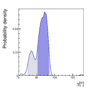
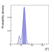
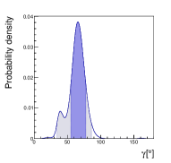
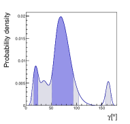
Figure 1: From left to right: P.d.f. for $\gamma$ obtained using the GL method as described in the text; p.d.f. for $\gamma$ obtained using the F method for $\kappa=0.1$, $0.3$, $0.5$. Here and in the following, dark (light) areas correspond to $68\%$ ($95\%$) probability regions.

We now consider the result of the combined GL+F analysis. In Fig. 2 we present the p.d.f. for $\gamma$ for $\kappa=0.1$, $0.3$ and $0.5$. We see that the result of the combined analysis is much more stable against the amount of U-spin breaking allowed. We also plot the $68\%$ probability region for $\gamma$ obtained using the combined method as a function of $\kappa$, and compare it to the GL result. We see that there is a considerable gain in precision even for gigantic values of $\kappa$. Actually, as can be seen in Fig. 3, where the posteriors for hadronic parameters and the U-spin breaking parameter $r_{C}$ are reported, the $68\%$ probability range for $r_{C}$ is between $\sim 0.4$ and $\sim 0.9$. The fact that the $r_{C}$ posterior is not centered around $1$, but the product $r_{C}r_{\mathrm{fact}}$ is close to $1$, may signal a failure of factorization and/or of the QCD sum rule estimate of $r_{\mathrm{fact}}$. On the other hand, the posteriors for $d^{\prime}$ and $\theta^{\prime}$ are well compatible with small U-spin breaking. In any case, we think that the lesson to be learned from Fig. 3 is that values of $\kappa$ up to $0.6$ or $0.7$ cannot be excluded, but nevertheless the combined method remains useful. This happens because the peak around $\gamma\sim 30^{\circ}$ in the GL result corresponds to values of $\theta$ that are different from the ones needed in the F analysis to obtain similar values of $\gamma$, while the peak at $\gamma\sim 70^{\circ}$ is obtained for the same values of hadronic parameters in both the GL and F analyses.

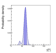
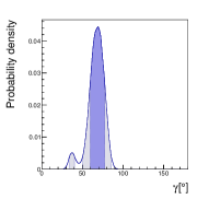
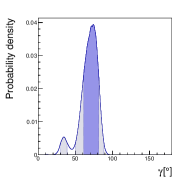
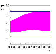
Figure 2: From left to right: P.d.f. for $\gamma$ obtained using the combined method for $\kappa=0.1$, $0.3$, $0.5$; $68\%$ probability region for $\gamma$ obtained using the combined method (filled area) or the GL method (horizontal lines) as a function of $\kappa$.

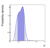
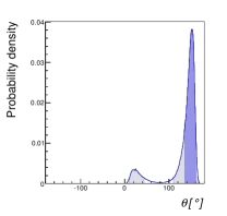
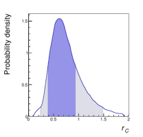
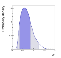
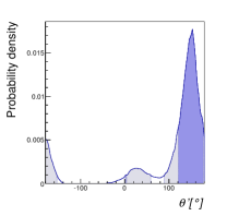
Figure 3: From left to right and from top to bottom: P.d.f. for $C$, $d$, $\theta$, $r_{C}$, $d^{\prime}$, $\theta^{\prime}$ obtained using the combined method for $\kappa=0.9$.

New Physics could affect the determination of $\gamma$ in the combined method by giving (electroweak) penguin contributions with a new CP-violating phase. Let us assume for concreteness that NP only enters $b\to s$ decays, so that the isospin analysis of the GL channels is still valid. In the framework of a global fit, one can simultaneously determine $\gamma$ and the NP contribution to $b\to s$ penguins. For the purpose of illustration, we can just use as input the value of $\gamma$ from tree-level processes, $\gamma_{\mathrm{tree}}=(76\pm 9)^{\circ}$ *[][andonlineupdateathttp://www.utfit.org/UTfit/ResultsSummer2011PostLP]Bona:2007vi, and look at the posterior for $\gamma$ and for the NP penguin amplitude. Taking for simplicity equal magnitudes for the NP contribution to $A(B_{s}\to K^{+}K^{-})$ and $A(\bar{B}_{s}\to K^{+}K^{-})$, we write

$$A(B_{s}\to K^{+}K^{-}) = C^{\prime}\frac{\lambda}{1-\lambda^{2}/2}(e^{i\gamma}+\frac{1-\lambda^{2}}{\lambda^{2}}(d^{\prime}e^{i\theta^{\prime}}+e^{i\phi_{\mathrm{NP}}^{\prime}}d^{\prime}_{\mathrm{NP}}e^{i\theta^{\prime}_{\mathrm{NP}}}))\,,$$ (6)

$$A(\bar{B}_{s}\to K^{+}K^{-}) = C^{\prime}\frac{\lambda}{1-\lambda^{2}/2}(e^{-i\gamma}+\frac{1-\lambda^{2}}{\lambda^{2}}(d^{\prime}e^{i\theta^{\prime}}+e^{-i\phi_{\mathrm{NP}}^{\prime}}d^{\prime}_{\mathrm{NP}}e^{i\theta^{\prime}_{\mathrm{NP}}}))\,.$$

Taking uniformly distributed $d^{\prime}_{\mathrm{NP}}\in[0,2]$ and $\phi^{\prime}_{\mathrm{NP}},\theta^{\prime}_{\mathrm{NP}}\in[-\pi,\pi]$ we obtain the p.d.f. reported in Fig. 4 for $\kappa=0.5$. It yields $\gamma=(74\pm 6)^{\circ}$, and a $95\%$ probability upper bound on $d^{\prime}_{\mathrm{NP}}$ around $1$. The bound is actually much stronger for large values of $\phi^{\prime}_{\mathrm{NP}}$.

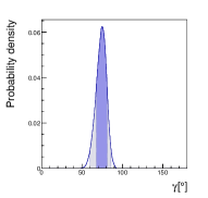
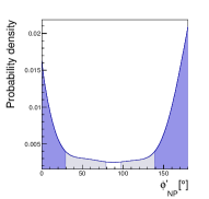
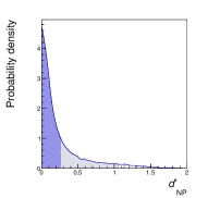
Figure 4: From left to right: P.d.f. for $\gamma$, $\phi_{\mathrm{NP}}^{\prime}$, $d^{\prime}_{\mathrm{NP}}$ and $\theta^{\prime}_{\mathrm{NP}}$ obtained using the combined method for $\kappa=0.5$.

Finally, we notice that $B_{s}\to KK$ decays can also be used to obtain information on $\phi_{M}(B_{s})$. The optimal choice in this respect is represented by $B_{s}\to K^{(*)0}\bar{K}^{(*)0}$ (with $B_{d}\to K^{(*)0}\bar{K}^{(*)0}$ as U-spin related control channel to constrain subleading contributions), since in this channel there is no tree contribution proportional to $e^{i\gamma}$ Ciuchini et al. (2008). However, the combined analysis described above, in the framework of a global SM fit, can serve for the same purpose. To illustrate this point, we perform the GL+F analysis not using the measurement of $2\beta_{s}$ from $b\to c\bar{c}s$ decays. In this way, we obtain $2\beta_{s}=(6\pm 14)^{\circ}$ for $\kappa=0.5$. With improved experimental accuracy, this determination will become competitive with the one from $b\to c\bar{c}s$ decays, since the theoretical uncertainty can be estimated more reliably in the case of $B_{s}\to K^{+}K^{-}$ decays, waiting for time-dependent analyses of the $B_{(s)}\to K^{(*)0}\bar{K}^{(*)0}$ channels. To illustrate the potential of this method, we have repeated the analysis reducing the experimental uncertainty on $A_{\mathrm{CP}}(B_{d}\to\pi^{+}\pi^{-})$, $S(B_{d}\to\pi^{+}\pi^{-})$, $A_{\mathrm{CP}}(B_{s}\to K^{+}K^{-})$ and $S(B_{s}\to K^{+}K^{-})$ down to $\pm 0.02$. With such small experimental errors, it becomes crucial to take correctly into account the effect of the subleading term proportional to $e^{i\gamma}$ in the amplitude (this is the case for any channel used to extract $\beta_{s}$ with an uncertainty of few degrees, including $B_{s}\to J/\psi\phi$). This is best done in the context of a global fit. For the purpose of illustration, we take as input the SM fit result $\gamma=(69.7\pm 3.1)^{\circ}$ *[][andonlineupdateathttp://www.utfit.org/UTfit/ResultsSummer2011PostLP]Bona:2007vi and obtain $2\beta_{s}=(2.6\pm 2.7)^{\circ}$ for $\kappa=0.5$. The error, which includes the theoretical uncertainty, could be further reduced improving the other relevant measurements, including the $B_{d}$ decay modes, and by adding the $B_{d,s}\to K^{(*)0}\bar{K}^{(*)0}$ channels, allowing to test the SM prediction for CP violation in $B_{s}$ mixing.

To conclude, let us summarize our findings. We suggest that the usual GL analysis to extract $\alpha$ from $B_{d}\to\pi\pi$ be supplemented with the inclusion of the $B_{s}\to K^{+}K^{-}$ modes, in the framework of a global CKM fit. The method optimizes the constraining power of these decays and allows to derive constraints on NP contributions to penguin amplitudes or on the $B_{s}$ mixing phase. We have illustrated these capabilities with a simplified analysis, neglecting correlations with other SM observables.

M.C. is associated to the Dipartimento di Fisica, Università di Roma Tre. E.F., S.M. and L.S. are associated to the Dipartimento di Fisica, Università di Roma “La Sapienza”. We acknowledge partial support from ERC Ideas Starting Grant n. 279972 “NPFlavour” and ERC Ideas Advanced Grant n. 267985 “DaMeSyFla”. We are indebted to Vincenzo Vagnoni for enlightening comments and suggestions and for pointing out to us the correction factor derived in ref. de Bruyn et al. (2012).

References

- Gronau and London (1990) M. Gronau and D. London, Phys.Rev.Lett. 65, 3381 (1990).
- Charles (1999) J. Charles, Phys.Rev. D59, 054007 (1999), arXiv:hep-ph/9806468 [hep-ph] .
- Bona et al. (2007) M. Bona et al. (UTfit Collaboration), Phys.Rev. D76, 014015 (2007), arXiv:hep-ph/0701204 [hep-ph] .
- Fleischer (1999) R. Fleischer, Phys.Lett. B459, 306 (1999), arXiv:hep-ph/9903456 [hep-ph] .
- Fleischer (2007) R. Fleischer, Eur.Phys.J. C52, 267 (2007), arXiv:0705.1121 [hep-ph] .
- Fleischer and Knegjens (2011) R. Fleischer and R. Knegjens, Eur.Phys.J. C71, 1532 (2011), arXiv:1011.1096 [hep-ph] .
- LHC (2012a) The LHCb Collaboration, LHCb-CONF-2012-007 (2012a).
- Beneke (2003) M. Beneke, eConf C0304052, FO001 (2003), arXiv:hep-ph/0308040 [hep-ph] .
- Ciuchini et al. (2005) M. Ciuchini, M. Pierini, and L. Silvestrini, Phys.Rev.Lett. 95, 221804 (2005), arXiv:hep-ph/0507290 [hep-ph] .
- Faller et al. (2009a) S. Faller, M. Jung, R. Fleischer, and T. Mannel, Phys.Rev. D79, 014030 (2009a), arXiv:0809.0842 [hep-ph] .
- Gronau and Rosner (2009) M. Gronau and J. L. Rosner, Phys.Lett. B672, 349 (2009), arXiv:0812.4796 [hep-ph] .
- Ciuchini et al. (2011) M. Ciuchini, M. Pierini, and L. Silvestrini, (2011), arXiv:1102.0392 [hep-ph] .
- Ciuchini et al. (2008) M. Ciuchini, M. Pierini, and L. Silvestrini, Phys.Rev.Lett. 100, 031802 (2008), arXiv:hep-ph/0703137 [hep-ph] .
- Faller et al. (2009b) S. Faller, R. Fleischer, and T. Mannel, Phys.Rev. D79, 014005 (2009b), arXiv:0810.4248 [hep-ph] .
- Aubert et al. (2008) B. Aubert et al. (BABAR Collaboration), (2008), arXiv:0807.4226 [hep-ex] .
- Ishino et al. (2007) H. Ishino et al. (Belle Collaboration), Phys.Rev.Lett. 98, 211801 (2007), arXiv:hep-ex/0608035 [hep-ex] .
- Aubert et al. (2007a) B. Aubert et al. (BABAR Collaboration), Phys.Rev. D75, 012008 (2007a), arXiv:hep-ex/0608003 [hep-ex] .
- Chang (2011) P. Chang, talk presented at EPS-HEP 2011 (2011).
- Bornheim et al. (2003) A. Bornheim et al. (CLEO Collaboration), Phys.Rev. D68, 052002 (2003), arXiv:hep-ex/0302026 [hep-ex] .
- Aaltonen et al. (2011) T. Aaltonen et al. (CDF Collaboration), Phys.Rev.Lett. 106, 181802 (2011), arXiv:1103.5762 [hep-ex] .
- Abe et al. (2005) K. Abe et al. (Belle Collaboration), Phys.Rev.Lett. 94, 181803 (2005), arXiv:hep-ex/0408101 [hep-ex] .
- Aubert et al. (2007b) B. Aubert et al. (BABAR Collaboration), Phys.Rev. D76, 091102 (2007b), arXiv:0707.2798 [hep-ex] .
- Peng et al. (2010) C.-C. Peng et al. (Belle Collaboration), Phys.Rev. D82, 072007 (2010), arXiv:1006.5115 [hep-ex] .
- Asner et al. (2010) D. Asner et al. (Heavy Flavor Averaging Group), (2010), arXiv:1010.1589 [hep-ex] .
- LHC (2012b) The LHCb Collaboration, LHCb-CONF-2012-002 (2012b).
- Gronau et al. (1999) M. Gronau, D. Pirjol, and T.-M. Yan, Phys.Rev. D60, 034021 (1999), arXiv:hep-ph/9810482 [hep-ph] .
- Zupan (2007) J. Zupan, Nucl.Phys.Proc.Suppl. 170, 33 (2007), arXiv:hep-ph/0701004 [hep-ph] .
- Gardner (2005) S. Gardner, Phys.Rev. D72, 034015 (2005), arXiv:hep-ph/0505071 [hep-ph] .
- Botella et al. (2006) F. Botella, D. London, and J. P. Silva, Phys.Rev. D73, 071501 (2006), arXiv:hep-ph/0602060 [hep-ph] .
- de Bruyn et al. (2012) K. de Bruyn, R. Fleischer, R. Knegjens, P. Koppenburg, M. Merk, et al., (2012), arXiv:1204.1735 [hep-ph] .
- Bona et al. (2008) M. Bona et al. (UTfit Collaboration), JHEP 0803, 049 (2008), arXiv:0707.0636 [hep-ph] .
- Aaij et al. (2012) R. Aaij et al. (LHCb Collaboration), Phys.Lett. B707, 349 (2012), arXiv:1111.0521 [hep-ex] .
- LHC (2012c) The LHCb Collaboration, LHCb-CONF-2012-001 (2012c).
- Duplancic and Melic (2008) G. Duplancic and B. Melic, Phys.Rev. D78, 054015 (2008), arXiv:0805.4170 [hep-ph] .
- Bhattacharya et al. (2012) B. Bhattacharya, A. Datta, M. Imbeault, and D. London, (2012), arXiv:1203.3435 [hep-ph] .