Analytical Continuation Approaches to Electronic Transport: The Resonant Level Model

Abstract

The analytical continuation average spectrum method (ASM) and maximum entropy (MaxEnt) method are applied to the dynamic response of a noninteracting resonant level model within the framework of the Kubo formula for electric conductivity. The frequency dependent conductivity is inferred from the imaginary time current-current correlation function for a wide range of temperatures, gate voltages and spectral densities representing the leads, and compared with exact results. We find that the MaxEnt provides more accurate results compared to the ASM over the full spectral range.

I Introduction

The computation of real time correlation functions in many-body quantum systems is challenging due to the exponential complexity of evaluating exact quantum dynamics.loh_sign_1990 ; yanagisawa_quantum_2007 ; bouadim_sign_2008 ; during_statistical_2010 This is exemplified by the well-known dynamical sign problem common to real-time Monte-Carlo techniques. The sign problem can be avoided in imaginary time and Wick rotation may be used to recover all the real time information and excitation spectra. However, since the imaginary time correlation function must be determined numerically via Quantum Monte Carlo (QMC),Berne86rb the rotation becomes numerically unstable and is highly sensitive to statistical errors.jarrell_bayesian_1996

Several approaches have been developed in order to circumvent this problem, such as the maximum entropy (MaxEnt) method where the optimal fitting of a data is defined in a Bayesian manner, which in general describes the competition between the $\chi^{2}$ goodness of the fit and an entropic prior $S$.jarrell_bayesian_1996 ; Krilov01c The MaxEnt approach has been applied successfully to a number of physically interesting problems.Gubernatis90 ; gubernatis_quantum_1991 ; gubernatis_quantum_1991-1 ; Berne94a ; Ceperley96 ; Berne96a ; Krilov99 ; Rabani00 ; Krilov01a ; Krilov01b ; Rabani02c ; Rabani03 ; Rabani05 ; Manolopoulos07 ; Miller08 ; Voth2008 A second approach is based on the notion of averaging over a sequences of possible solutions. Such approach is called stochastic analytical continuation method or average spectrum methods (ASM).sandvik_stochastic_1998 ; assaad_spin_2008 ; syljuasen_using_2008 ; kletenik-edelman_analytic_2010 Recent application of the ASM and MaxEnt approaches argued that the ASM should be superior to the MaxEnt at least in its ability to resolve sharp spectral features.vitali_path-integral_2008 ; reichman_analytic_2009 Examples included the calculation of the dynamical density fluctuations in liquid para-hydrogen and ortho-deuterium reichman_analytic_2009 as well as spin dynamics in anti ferromagnetic Heisenberg spin chain.syljuasen_using_2008

In this work we apply both methods to study the dynamic response of the well known resonant level model stovneng_buttiker-landauer_1989 and exhibit the dc conductivity extracted from these approaches as well its frequency dependence. Our approach to describe the conductivity is quite different from that discussed recently in the literature,Han2010 in that it is not limited to a specific choice of the Hamiltonian; it does however, apply to equilibrium situations only. To assess the accuracy of both analytic continuation methods, we compare the results to the exact solution, which predicts a smooth broad spectrum. We find the MaxEnt approach provides an overall good agreement with the exact solution for the entire range of frequencies and is particularly accurate at low frequencies near the dc regime. On the other hand, the ASM yields sharp, narrowed spectral features as well as spurious concave domains which are noticeably different from the exact results. Moreover, its low frequency predictions are somewhat less accurate compared to those of the MaxEnt method.

The paper is organized as follows: In Section II we describe an analytic continuation approach for electrical conductivity and briefly review two techniques to perform the Wick rotation: The ASM and the MaxEnt method. In Section III we describe our model Hamiltonian and the exact solution for the electrical conductivity within Kubo’s linear response theory. Section IV is devoted to present the results obtained from the ASM and MaxEnt approaches. Conclusions are given in Section V.

II Analytical Continuation

The objective is to obtain the electrical conductivity from Kubo’s linear response theory:kubo_statistical-mechanical_1957

$$\sigma_{\kappa}(\omega)=\beta\int_{0}^{\infty}dte^{-i\omega t}\langle\hat{I}(t)\hat{I}(0)\rangle_{\kappa}$$ (1)

where $\beta=\frac{1}{k_{\mbox{\tiny B}}T}$ is the inverse temperature, $\hat{I}$ is the current operator defined below (see Eq. 14), and the label $\langle\cdots\rangle_{\kappa}$ represents the Kubo transform of the current-current correlation function defined by:kubo_statistical-mechanical_1957

$$\langle\hat{I}(t)\hat{I}(0)\rangle_{\kappa}\equiv\frac{1}{\beta\hbar}\int_{0}^{\beta\hbar}d\lambda\langle\hat{I}(t-i\lambda)\hat{I}(0)\rangle.$$ (2)

In the above, $\hbar$ is the reduced Planck’s constant and $\langle\cdots\rangle$ denotes an ensemble average.

To obtain the electrical conductivity, one requires the calculation of the current-current correlation function, $C\left(t\right)=\langle\hat{I}(t)\hat{I}(0)\rangle$, in real time:

$$C\left(t\right)=\frac{1}{Q}Tr\left\{e^{-\beta\hat{H}}e^{\frac{it}{\hbar}\hat{H}}\hat{I}e^{-\frac{it}{\hbar}\hat{H}}\hat{I}\right\},$$ (3)

where $\hat{H}$ is the Hamiltonian of the problem and $Q$ the canonical partition function. $C\left(t\right)$ is related to the frequency response function $D\left(\omega\right)$ by a simple Fourier relation:

$$C\left(t\right)=\frac{1}{2\pi}\overset{\infty}{\underset{-\infty}{\int}}e^{-i\omega t}D\left(\omega\right)d\omega.$$ (4)

The frequency response function, $D\left(\omega\right)$, can be written in terms of the real part of the electrical conductivity, $\sigma_{\kappa}(\omega)$:

$$D\left(\omega\right)=\hbar\omega\left(1+\coth\left(\frac{\beta\hbar\omega}{2}\right)\right)\Re\{\sigma_{\kappa}\left(\omega\right)\},$$ (5)

where for $\omega\rightarrow 0$, the dc conductivity is given by ($\Im\{\sigma_{\kappa}\left(\omega\rightarrow 0\right)\}=0$):

$$\sigma_{\kappa}\left(0\right)=\frac{\beta}{2}D\left(0\right).$$ (6)

To obtain $\sigma\left(\omega\right)$, one requires the direct calculation of $C\left(t\right)$, which is an extremely difficult task for a typical model Hamiltonian used to describe transport in confined systems. However, in comparison the real time case, the calculate the corresponding imaginary-time function by QMC techniques is less tedious.Ceperley95 In imaginary time, the corresponding autocorrelation function is also related to $D\left(\omega\right)$. This relation is achieved by performing the Wick rotation, replacing $t\rightarrow-i\tau$ and using the detailed balance relation $D\left(-\omega\right)=e^{-\beta\hbar\omega}D\left(\omega\right)$:

$$C\left(-i\tau\right)=\frac{1}{2\pi}\underset{0}{\overset{\infty}{\int}}\left(e^{\left(\tau-\beta\hbar\right)\omega}+e^{-\omega\tau}\right)D\left(\omega\right)d\omega,$$ (7)

where $0\leq\tau\leq\hbar\beta$ and the imaginary time autocorrelation function can be calculated by modifying the Heisenberg equation of motion in Eq. (3):

$$C\left(-i\tau\right)=\frac{1}{Q}Tr\left\{e^{-\beta\hat{H}}e^{\frac{\tau}{\hbar}\hat{H}}\hat{I}e^{-\frac{\tau}{\hbar}\hat{H}}\hat{I}\right\}.$$ (8)

Much of the difficulty in calculating $C\left(t\right)$ is now shifted to that of inverting the above relation to obtain $D(\omega)$ from $C(-i\tau)$. We refer to two approaches developed to invert this relation: The MaxEnt method and the ASM. The MaxEnt method selects the solution which maximizes the posterior probability, or the probability of the solution $D(\omega)$ given a data set $C(-i\tau)$. Using Bayes’ theorem, one can show that the posterior probability is given by Gubernatis91 ; Skilling89

$${\cal{P}}(D(\omega)|C(-i\tau))\propto\exp(\alpha S-\chi^{2}/2).$$ (9)

where $S$ is the information entropy and $\chi^{2}$ is the standard mean squared deviation from the data. In the present study, we only consider the standard L-curve method to determine $\alpha$.Lawson95 In this context we regard $\alpha$ as a regularization parameter controlling the degree of smoothness of the solution, and the entropy as the regularizing function. Its value is selected by constructing a plot of $\log[-S]$ vs. $\log\chi^{2}$. This curve has a characteristic L-shape, and the corner of the L, or the point of maximum curvature, corresponds to the value of $\alpha$ which is the best compromise between fitting the data and obtaining a smooth solution. Our experience with analytic continuation has lead us to the conclusion that this approach is the most robust. Once the regularization parameter is determined, we apply the approach described in Ref. Krilov01c, to obtain the statistically rigorous and unique fit for $D(\omega)$.

The basic idea behind the ASM is to pick the final solution for $D(\omega)$ as the average spectral function obtained by averaging over a posterior probability, ${\cal{P}}(D(\omega)|C(-i\tau))$, instead of taking the value that maximizes this distribution. Thus, fluctuations of the solution are allowed in the ASM:

$$\bar{D}(\omega)=\frac{\int d|D(\omega)|D(\omega){\cal{P}}(D(\omega)|C(-i\tau))}{\int d|D(\omega)|{\cal{P}}(D(\omega)|C(-i\tau))}.$$ (10)

The averaging is performed by a Monte Carlo procedure preserving known sum rules.reichman_analytic_2009 Readers who are interested in a more comprehensive discussion of the ASM are referred to Refs. Sandvik98, and Syljuasen08, and to the specific implementation of Ref. reichman_analytic_2009, .

III Model

We consider the resonant Level model, which consists of a single quantum dot state coupled to two leads (fermionic baths). This model has been used extensively in understanding transport properties of non-interacting systems, most recently in a semiclassical study of transport developed by Swenson et al.swenson_application_2011 Since an exact solution of the frequency dependent conductivity is available, this model is ideal for assessing the accuracy of the proposed analytic continuation approach. The Hamiltonian is given by (more details can be found in Ref. swenson_application_2011, )

$$\hat{H}=\varepsilon_{d}d^{\dagger}d+\underset{k\in L,R}{\sum}\varepsilon_{k}c_{k}^{\dagger}c_{k}+\underset{k\in L,R}{\sum}t_{k}\left(d^{\dagger}c_{k}+h.c.\right),$$ (11)

where $d$ ($d^{\dagger}$) is the destruction (creation) operator of an electron on the dot, $\varepsilon_{d}$ is the energy of the isolated dot (which will also be referred to as the gate potential), $c_{k}$ ($c_{k}^{\dagger}$) is the destruction (creation) operator of an electron on the left (L) or right (R) lead with energy $\varepsilon_{k}$, and $t_{k}$ is the coupling amplitude between the dot and the lead level $k$.

For a full specification of the model, one requires the spectral function which determines $t_{k}$. In the applications reported below, the leads will be described within the wide band limit with a sharp cutoff at high and low energy values, such that the spectral density is given by

$$J_{L/R}\left(\varepsilon\right)=\frac{\Gamma_{L/R}}{\left(1+e^{A\left(\varepsilon-B\right)}\right)\left(1+e^{-A\left(\varepsilon+B\right)}\right)}$$ (12)

In the calculations reported below, unless otherwise noted, we use $\Gamma_{L}=\Gamma_{R}=\frac{1}{2}$, $\Gamma=\Gamma_{L}+\Gamma_{L}$, $A=5\Gamma$,$B=3-10\Gamma$. We also use a uniform discretization ($\delta\varepsilon_{K}$) to select the energies of the leads’ states, and thus the couplings are given by:

$$t_{k}\left(\varepsilon_{k}\right)=\sqrt{\frac{J\left(\varepsilon_{k}\right)\Delta\varepsilon_{k}}{2\pi}}.$$ (13)

Our aim is to use the ASM and MaxEnt method to calculate the measurable dc conductivity and its frequency dependence and compare the analytic continuation approaches to exact results. For the model Hamiltonian given above, the current operator, $\hat{I}$, is taken to represent the current from the left lead to the dot (similarly, one can look at the right current), and is given by the change in occupancy of the left lead, $\hat{I}=e\frac{d\hat{N}_{L}}{dt}$, where $\hat{N}_{L}=\underset{k\in L}{\sum}c_{k}^{\dagger}c_{k}$, and a brief calculations shows that

$$\hat{I}=\frac{ie}{\hbar}\underset{k\in L}{\sum}t_{k}\left(c_{k}^{\dagger}d-d^{\dagger}c_{k}\right).$$ (14)

With the above definition, the current-current correlation function can be calculated exactly in order to obtain the conductivity based on Kubo’s linear response theory.kubo_statistical-mechanical_1957 Let us assume that one knows the matrix which diagonalizes the Hamiltonian in Eq. (11) and denote it by $U$. By making a linear transformation for the operators $c_{k}=\underset{\alpha}{\sum}U_{k\alpha}\tilde{c}_{\alpha}$ and $c_{k}^{\dagger}=\underset{\alpha}{\sum}U_{\alpha k}^{-1}\tilde{c}_{\alpha}^{\dagger}$ (where from now on the index $k=0$ will be refereed to that of the dot level), we can rewrite the expression for $C\left(t\right)$ in terms of the eigenfunctions of diagonal Hamiltonian:

$$C\left(t\right) = \frac{1}{Q}Tr\left\{e^{-\beta\hat{H}}e^{i\hat{H}\frac{t}{\hbar}}\hat{I}e^{-i\hat{H}\frac{t}{\hbar}}\hat{I}\right\}$$ (15)

$$= \frac{e^{2}}{\hbar^{2}}\underset{nm}{\sum}e^{i\left(\tilde{\varepsilon}_{n}-\tilde{\varepsilon}_{m}\right)\frac{t}{\hbar}}\Xi{}_{nm}^{2}f\left(\tilde{\varepsilon}_{n}\right)\left[1-f\left(\tilde{\varepsilon}_{m}\right)\right].$$

In the above, $\tilde{\varepsilon}_{n}$ are the energy eigenvalues from the diagonalized Hamiltonian $\tilde{H}=\overset{\infty}{\underset{i=0}{\sum}}\tilde{\varepsilon}_{i}\tilde{c}_{i}^{\dagger}\tilde{c}_{i}$, $f\left(\tilde{\varepsilon}_{n}\right)$ are the Fermi-Dirac distribution at equilibrium, and

$$\Xi{}_{nm}^{2}=\underset{q,k}{\sum}t_{k}t_{q}\left(U_{m0}^{-1}U_{kn}-U_{mk}^{-1}U_{0n}\right)\left(U_{m0}^{-1}U_{qn}-U_{mq}^{-1}U_{0n}\right)$$ (16)

can be refereed to as the electron velocity matrix element in the the orthogonal basis, which obeys $\Xi_{nn}=0$ for the same quantum state. The Fourier transform of Eq. (15) gives

$$D\left(\omega\right) = \underset{\eta\rightarrow 0^{+}}{\lim}\frac{2\pi e^{2}}{\hbar}\underset{nm}{\sum}\Xi_{nm}^{2}\frac{e^{\beta\tilde{\varepsilon}_{n}}f\left(\tilde{\varepsilon}_{n}\right)}{e^{\beta\left(\tilde{\varepsilon}_{n}-\hbar\omega\right)}+1}\delta_{\eta}(\Delta_{nm}+\hbar\omega),$$

where $\Delta_{nm}=\tilde{\varepsilon}_{n}-\tilde{\varepsilon}_{m}$ and $\delta_{\eta}(x)$ is defined by

$$\delta_{\eta}(x)=\frac{1}{\pi}\frac{\hbar\eta}{x^{2}+\left(\hbar\eta\right)^{2}}.$$ (18)

Using Eq. (5), the experimental measured electrical conductivity can be calculated and is given by:

$$\Re\left\{\sigma_{\kappa}\left(\omega\right)\right\} = \underset{\eta\rightarrow 0^{+}}{\lim}\frac{e^{2}}{\hbar^{2}}\underset{nm}{\sum}\Xi_{nm}^{2}\frac{\Delta f_{mn}}{\Delta_{mn}}\delta_{\eta}(\Delta_{nm}+\hbar\omega)$$

(19)

where $\Delta f_{mn}=f\left(\tilde{\varepsilon}_{m}\right)-f\left(\tilde{\varepsilon}_{n}\right)$. In practice, we use a finite value of $\eta$ since the leads (baths) are described by a finite set of modes. We take $\hbar\eta$ to be larger than the spacing between adjacent bath modes and smaller than the band width. Its actual value is determined by starting from a large value of $\eta$ and gradually decreasing it until convergence occurs.imry_introduction_2002

Formally, for an infinite number of bath modes one can take the limit $\eta\rightarrow 0^{+}$:imry_introduction_2002

$$\Re\left\{\sigma_{\kappa}\left(\omega\right)\right\} = \frac{\pi e^{2}}{2\hbar}\frac{\sinh\left(\frac{\beta\hbar\omega}{2}\right)}{\hbar\omega}\underset{nm}{\sum}\Xi_{nm}^{2}$$ (20)

$$\,\times\mbox{sech}\left(\frac{\beta\tilde{\varepsilon}_{m}}{2}\right)\mbox{sech}\left(\frac{\beta\left(\tilde{\varepsilon}_{m}-\hbar\omega\right)}{2}\right)$$

$$\,\times\delta(\tilde{\varepsilon}_{n}-\tilde{\varepsilon}_{m}+\hbar\omega),$$

and the dc conductivity is then obtain by taking $\omega$ to $0$, which gives the well known Landauer formula for conductance datta_electronic_1997 ; datta_quantum_2005

$$\sigma_{\kappa}(0)=\frac{\pi e^{2}}{4\hbar}\beta\underset{nm}{\sum}\Xi_{nm}^{2}\mbox{sech}^{2}\left(\frac{\beta\tilde{\varepsilon}_{m}}{2}\right)\delta(\tilde{\varepsilon}_{n}-\tilde{\varepsilon}_{m}).$$ (21)

IV Results

The application of the ASM and MaxEnt method requires as input the imaginary time current-current correlation function, $C(-i\tau)$ given by Eq. 8. In principle, the calculation of such correlation functions requires numerical techniques such as those based on path integration, where a variety of approaches can be extended to imaginary time.hirsch_monte_1986 ; werner_continuous-time_2006 ; muehlbacher_real-time_2008 ; weiss_iterative_2008 ; werner_diagrammatic_2009 ; schiro_real-time_2009 ; segal_numerically_2010 ; werner_weak-coupling_2010 ; Gull10 In the present case, due to the simplicity of the model Hamiltonian (cf., Eq. (11)), instead of referring to a specific numerical implementation of a path integration approach, we derive an exact expression for $C(-i\tau)$. To preform the analytic continuation based on the ASM and MaxEnt method, we add artificial noise to the exact expression of $C(-i\tau)$ to mimic the results of a Monte Carlo procedure, as described below.

For a finite value of $\eta$ (see the discussion above), the imaginary time current-current correlation function is given by the exact expression:

$$C_{\eta}(\tau) = -\frac{ie^{2}}{2\pi\hbar^{2}}\underset{nm}{\sum}\Lambda_{nm}\left(e^{\Omega_{mn}\tau}E_{1}\left(\Omega_{mn}\tau\right)-e^{\Omega_{mn}^{*}\tau}E_{1}\left(\Omega_{mn}^{*}\tau\right)\right.$$ (22)

$$\left.+e^{\Omega_{mn}^{*}(\beta\hbar-\tau)}\left\{E_{i}\left(\Omega_{mn}^{*}(\tau-\beta\hbar)\right)+i\pi\right\}+ie^{\Omega_{mn}(\beta\hbar-\tau)}\left\{\pi+iE_{i}\left(\Omega_{mn}(\tau-\beta\hbar)\right)\right\}\right)$$

where $\Omega_{mn}=\frac{\tilde{\varepsilon}_{m}-\tilde{\varepsilon}_{n}-i\hbar\eta}{\hbar},\,\,\Lambda_{nm}=\Xi_{nm}^{2}f({\tilde{\varepsilon}_{m}})f({\tilde{\varepsilon}_{n}})e^{\beta\tilde{\varepsilon}_{n}}$, and $E_{i}\left(x\right)=-\underset{-x}{\overset{\infty}{\int}}\frac{e^{-t}}{t}dt,\,\,\,E_{n}\left(x\right)=-\underset{1}{\overset{\infty}{\int}}\frac{e^{-xt}}{t^{n}}dt$ are the exponential integral function and the $n^{\mbox{\tiny{th}}}$ exponential integral function, respectively. The above expression for $C_{\eta}(\tau)$ is well defined for $0\leq\tau\leq\hbar\beta$ and reduces to

$$C(-i\tau)\equiv C_{\eta\rightarrow 0^{+}}\left(\tau\right)=\frac{e^{2}}{\hbar^{2}}\underset{nm}{\sum}e^{\left(\tilde{\varepsilon}_{n}-\tilde{\varepsilon}_{m}\right)\frac{\tau}{\hbar}}\Lambda_{nm}$$ (23)

in the limit of $\eta\rightarrow 0^{+}$.

In Fig. 1 we plot the current-current correlation function in imaginary time for two values of $\beta$. The results were obtained for a finite number of bath modes ($N_{b}$), where $N_{b}=1000$ for both the left ($L$) and right ($R$) leads. The results are shown for $\hbar\eta=0.04\Gamma$. However, we find that within the accuracy of the numerical analytic continuation, the inversion is not sensitive to the value of $\eta$. In fact, on the scale of the plots shown in Fig. 1, different values of $\eta$ (within a reasonable range) are indistinguishable. This implies that one can refer to Monte Carlo simulations to obtain the imaginary time data for a finite number of bath modes and ignore the role of $\eta$ in the simulations. This, of course, is not the case in real time, where for a finite system $\sigma_{\kappa}(\omega=0)\rightarrow 0$ when $\eta=0$.imry_introduction_2002

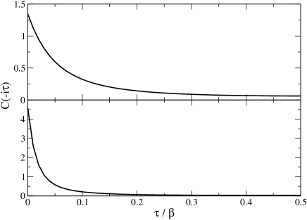
Figure 1: Current-current correlation function in imaginary time (cf., Eq. (22) for $\beta=3/\Gamma$ (upper panel) and $\beta=10/\Gamma$ (lower panel). Results are shown for $\hbar\eta=0.04\Gamma$ and $\epsilon_{d}=0$. On the scale of the plots, it is difficult to differentiate between results obtained for different values of $\eta$.

Next, we applied both the ASM and MaxEnt method to invert the imaginary time data. We added Gaussian noise to the imaginary time current-current correlation function with a standard deviation of $1\%$ at each data point. We discretized the imaginary time axis to $N_{\tau}=100$ points and the frequency axis to $N_{\omega}=1024$ points. For the ASM approach, we averaged the solution over $10^{7}$ Monte Carlo sweeps. In Fig. 2 we plot the results for the frequency dependent electrical conductivity at a gate voltage $\varepsilon_{d}=0$ and $\varepsilon_{d}=\Gamma$, and for two inverse temperatures of $\beta=\frac{3}{\Gamma}$ and $\beta=\frac{10}{\Gamma}$.

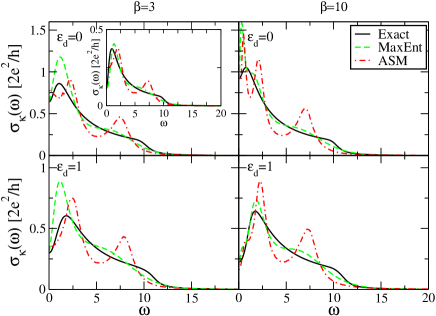
Figure 2: Frequency dependent electrical conductivity $\sigma_{\kappa}(\omega)$ obtained from the exact result from Eq. (19) (solid black curve), the ASM (dashed-dotted red curve) and the MaxEnt (dashed green curve) for different gate voltages $\left(\varepsilon_{d}\right)$ and temperatures. $\epsilon_{d}$ is denoted in units of $\Gamma$, $\beta$ in units of $1/\Gamma$, and $\omega$ in units of $\Gamma/\hbar$. Inset: Frequency dependent electrical conductivity $\sigma_{\kappa}(\omega)$ for the asymmetric coupling case $\Gamma_{L}=\frac{1}{2}$ and $\Gamma_{R}=\frac{1}{10}$.

We find that the MaxEnt provides an overall better agreement with the exact results compared to the ASM. Both approaches provide reasonable description at low frequencies, and thus are accurate enough to determine the dc conductivity (see below), though MaxEnt is in general more accurate in this spectral regime. Both approaches over-estimate the magnitude of the first peak observed at low frequencies. In general, MaxEnt does provide a better estimate of the position, height and width of the peak for the range of model parameters studied in this work. The ASM also produces a sharp peak at higher frequencies which does not appear in the exact solution for $\sigma_{\kappa}(\omega)$, while MaxEnt performs better in this regime. In fact, the high frequency behavior is quite tough for analytic continuation approaches. In $D(\omega)$ (not shown) we observe a sharp fall of the response as the frequency approaches the band cutoff $B$. This is translated to a small shoulder observed at $\hbar\omega=B$ in $\sigma(\omega)$. Such a sharp change in the spectral behavior is challenging for the analytic continuation methods, and this explains the failure of the ASM.

The inset of Fig. 2 shows a typical result for the asymmetric coupling case, where $\Gamma_{L}=\frac{1}{2}$ and $\Gamma_{R}=\frac{1}{10}$. This case is more difficult for analytic continuation since the overall magnitude of the conductivity is much smaller, due to the occurrence of destructive interference on the dot. MaxEnt provides reasonable results at all frequencies while the ASM fails markedly even at low frequencies. The fact that MaxEnt captures the behavior of the conductivity for the asymmetric case is encouraging. In fact, it suggests that the MaxEnt approach can be used for more elaborate situations: For example, when the coupling to the left lead is not proportional to that of the right lead and the simple Landauer type Meir-Wingreen formula is not adequate (see Eq. (9) in Ref. meir_landauer_1992, ).

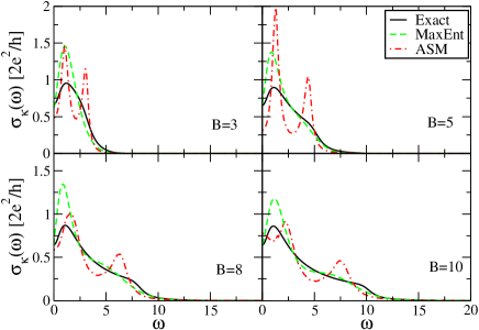
Figure 3: Same as Fig. 2 but for different values of the lead cutoff parameter, $B$, given in units of $\Gamma$.

The high frequency behavior is also determined by the band structure of the leads. In Fig. 3 we plot the frequency dependent electrical conductivity for different values of the band cutoff parameters, $B$ defined in Eq. (12). Indeed, the MaxEnt method gives a well behaved spectral response while the ASM provides two peaks for all values of $B$. This is even more pronounced at small values of $B$, where the width of the peaks in the ASM are very narrow, in contrast to the exact response which is smooth. Moreover, even the low frequency response of the ASM significantly deviates from the exact results at low band width, while within MaxEnt the accuracy at low frequency remains the same for all values of $B$, and the dc conductivity is only slightly affected by changing $B$.

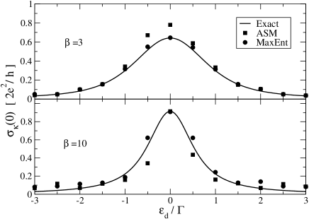
Figure 4: The dc conductivity $\sigma_{\kappa}(\omega=0)$ as a function of the gate voltage $\epsilon_{d}$ for temperature $\beta=3/\Gamma$ (upper panel) and $\beta=10/\Gamma$ (lower panel).

The dc conductivity as a function of the gate voltage and inverse temperature is shown in Fig. 4 and Fig. 5, respectively. The exact results given by Eq. (19) agree with the Landauer formula (not shown).imry_introduction_2002 For the current set of parameters, both approaches provide good results for the conductivity at $\omega=0$. Again, the MaxEnt method seems to provide more accurate results near the resonance and is quantitative for most gate voltages and temperatures.

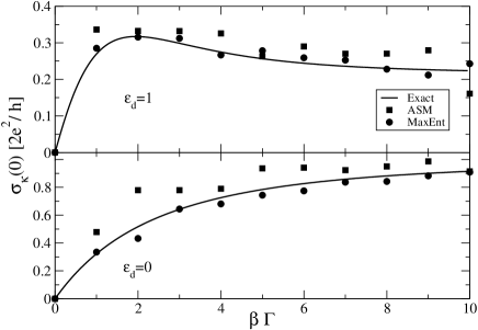
Figure 5: The dc conductivity as a function of the inverse temperature for gate voltage $\varepsilon_{d}=\Gamma$ (upper panel) and $\varepsilon_{d}=0$ (lower panel).

V Conclusions

We have presented an analytic continuation approach based on Kubo’s linear response theory to obtain the dc and ac components of the electrical conductivity in molecular junctions. Kubo’s formulation requires the calculation of the current-current correlation function in real time, which is a difficult task for a many-body open quantum system due to the well-known dynamical sign problem. The calculation of the corresponding imaginary time correlation, on the other hand, is a much simpler task, amenable to Monte Carlo techniques.

Two approaches were adopted here to carry the analytic continuation of the current-current correlation function to real time: the ASM and the MaxEnt method. To assess the accuracy of these methods, we performed calculations for the resonant level model at a wide range of temperatures, gate voltages and frequencies. The numerical results were compared with an exact expression for the electrical conductivity, which is straightforward to obtain for this model.

We find that MaxEnt is superior to the ASM for the entire range of frequencies and for different model parameters. It provides an accurate description of the dc conductivity as well as a reasonable approximation for the ac component. Furthermore, MaxEnt captures interference effects on the dot resulting from breaking the symmetry in the couplings between the dot and the leads. The ASM fails in all these respects.

VI Acknowledgments

We would like to thank Guy Cohen for helpful discussions and critical comments on the manuscript. EYW would like to thank Dr. Kalman Wilner for useful discussions. This work was supported by the US-Israel Binational Science Foundation and by the FP7 Marie Curie IOF project HJSC. TJL is grateful to the The Center for Nanoscience and Nanotechnology at Tel Aviv University of a doctoral fellowship.

References

- (1) E. Y. Loh, J. E. Gubernatis, R. T. Scalettar, S. R. White, D. J. Scalapino, and R. L. Sugar, Phys. Rev. B 41, 9301 (May 1990).
- (2) T. Yanagisawa, Phys. Rev. B 75, 224503 (June 2007).
- (3) K. Bouadim, M. Enjalran, F. Hébert, G. G. Batrouni, and R. T. Scalettar, Phys. Rev. B 77, 014516 (January 2008).
- (4) G. Düring and J. Kurchan, Europhys. Lett. 92, 50004 (December 2010).
- (5) B. J. Berne and D. Thirumalai, Ann. Rev. Phys. Chem. 37, 401 (1986).
- (6) M. Jarrell and J. Gubernatis, Phys. Rep. 269, 133 (May 1996).
- (7) G. Krilov, E. Sim, and B. J. Berne, Chem. Phys. 268, 21 (2001).
- (8) R. N. Silver, D. S. Sivia, and J. E. Gubernatis, Phys. Rev. B 41, 2380 (1990).
- (9) J. E. Gubernatis, M. Jarrell, R. N. Silver, and D. S. Sivia, Phys. Rev. B 44, 6011 (1991).
- (10) J. E. Gubernatis, M. Jarrell, R. N. Silver, and D. S. Sivia, Phys. Rev. B 44, 6011 (1991).
- (11) E. Gallicchio and B. J. Berne, J. Chem. Phys. 101, 9909 (1994).
- (12) M. Boninsegni and D. M. Ceperley, J. Low Temp. Phys. 104, 339 (1996).
- (13) E. Gallicchio and B. J. Berne, J. Chem. Phys. 105, 7064 (1996).
- (14) G. Krilov and B. J. Berne, J. Chem.Phys. 111, 9147 (1999).
- (15) E. Rabani, G. Krilov, and B. J. Berne, J. Chem. Phys. 112, 2605 (2000).
- (16) G. Krilov, E. Sim, and B. J. Berne, J. Chem. Phys. 114, 1075 (2001).
- (17) E. Sim, G. Krilov, and B. J. Berne, J. Phys. Chem. 105, 2824 (2001).
- (18) E. Rabani, D. R. Reichman, G. Krilov, and B. J. Berne, Proc. Natl. Acad. Sci. USA 99, 1129 (2002).
- (19) A. A. Golosov, D. R. Reichman, and E. Rabani, J. Chem. Phys. 118, 457 (2003).
- (20) E. Rabani, G. Krilov, D. R. Reichman, and B. J. Berne, J. Chem. Phys. 123, 184506 (2005).
- (21) S. Habershon, B. J. Braams, and D. E. Manolopoulos, J. Chem. Phys. 127, 174108 (2007).
- (22) J. Liu and W. H. Miller, J. Chem. Phys. 129, 124111 (2008).
- (23) F. Paesani and G. A. Voth, J. Chem. Phys. 129, 194113 (2008).
- (24) A. W. Sandvik, Phys. Rev. B 57, 10287 (May 1998).
- (25) F. F. Assaad, Phys. Rev. B 78, 155124 (October 2008).
- (26) O. F. Syljuåsen, Phys. Rev. B 78, 174429 (November 2008).
- (27) O. Kletenik-Edelman, E. Rabani, and D. R. Reichman, Chem. Phys. 370, 132 (May 2010).
- (28) E. Vitali, M. Rossi, F. Tramonto, D. E. Galli, and L. Reatto, Phys. Rev. B 77, 180505 (May 2008).
- (29) D. R. Reichman and E. Rabani, J. Chem. Phys. 131, 054502 (August 2009).
- (30) J. A. Støvneng and E. H. Hauge, J. Stat. Phys. 57, 841 (1989).
- (31) J. E. Han, Phys. Rev. B 81, 245107 (2010).
- (32) R. Kubo, J. Phys. Soc. Japan 12, 570 (1957).
- (33) D. M. Ceperley, Rev. Mod. Phys. 67, 279 (1995).
- (34) J. E. Gubernatis, M. Jarrell, R. N. Silver, and D. S. Sivia, Phys. Rev. B 44, 6011 (1991).
- (35) J. Skilling, editor, Maximum Entropy and Bayesian Methods (Kluwer, Cambridge, England, 1989).
- (36) C. L. Lawson and R. J. Hanson, Solving Least Squares Problems (Society for Industrial and Applied Mathematics, 1995).
- (37) A. W. Sandvik, Phys. Rev. B 57, 10287 (1998).
- (38) O. F. Syljuasen, Phys. Rev. B 78, 174429 (2008).
- (39) D. W. H. Swenson, T. Levy, G. Cohen, E. Rabani, and W. H. Miller, J. Chem. Phys. 134, 164103 (2011).
- (40) Y. Imry, Introduction to mesoscopic physics (Oxford University Press, 2002).
- (41) S. Datta, Electronic Transport in Mesoscopic Systems (Cambridge University Press, 1997).
- (42) S. Datta, Quantum Transport: Atom To Transistor (Cambridge University Press, 2005).
- (43) J. E. Hirsch and R. M. Fye, Phys. Rev. Lett. 56, 2521 (June 1986).
- (44) P. Werner, A. Comanac, L. deMedici, M. Troyer, and A. J. Millis, Phys. Rev. Lett. 97, 076405 (2006).
- (45) L. Mühlbacher and E. Rabani, Phys. Rev. Lett. 100, 176403 (2008).
- (46) S. Weiss, J. Eckel, M. Thorwart, and R. Egger, Phys. Rev. B 77, 195316 (2008).
- (47) P. Werner, T. Oka, and A. J. Millis, Phys. Rev. B 79, 035320 (January 2009).
- (48) M. Schiró and M. Fabrizio, Phys. Rev. B 79, 153302 (2009).
- (49) D. Segal, A. J. Millis, and D. R. Reichman, Phys. Rev. B 82, 205323 (2010).
- (50) P. Werner, T. Oka, M. Eckstein, and A. J. Millis, Phys. Rev. B 81, 035108 (January 2010).
- (51) E. Gull, D. R. Reichman, and A. J. Millis, Phys. Rev. B 82, 075109 (2010).
- (52) Y. Meir and N. S. Wingreen, Phys. Rev. Lett. 68, 2512 (April 1992).