Signed Simplicial Decomposition and Overlay of $n$-D Polytope Complexes

Abstract

Polytope complexes are the generalisation of polygon meshes in geo-information systems (GIS) to arbitrary dimension, and a natural concept for accessing spatio-temporal information. Complexes of each dimension have a straight-forward dimension-independent database representation called Relational Complex. Accordingly, complex overlay is the corresponding generalisation of map overlay in GIS to arbitrary dimension. Such overlay can be computed by partitioning the cells into simplices, intersecting these and finally combine their intersections into the resulting overlay complex. Simplex partitioning, however, can expensive in dimension higher than $2$. In the case of polytope complex overlay signed simplicial decomposition is an alternative. This paper presents a purely combinatoric polytope complex decomposition which ignores geometry. In particular, this method is also a decomposition method for non-convex polytopes. Geometric $n$-D-simplex intersection is then done by a simplified active-set-method—a well-known numerical optimisation method. “Summing” up the simplex intersections then yields the desired overlay complex.

1 Introduction

An important query operation in GIS is the overlay of some given “topologies” to generate new such “topologies”. An example could be cadastral land-owner data overlaid with environmental stress data which helps to identify which owner is affected by what averse environmental influences. This operation seems to be missing in 3D cadastral applications:

However, 3D data management and analysis such as querying, manipulation, 3D map overlay, 3D buffering have been largely neglected in spatial database systems and Geographic Information Systems. Streilein:3DDataManagement

To compute such overlay by first triangulate the input, then overlay these triangles and finally recombine the resulting intersections into the desired overlay complex is possible in $2$-d, but such triangulation in $3$-d, however, has $\Omega(n^{2})$ space complexity in general Chazelle:ConvexPartitions and, hence, is very expensive.

The special case of convex $3$-d-shapes, however, is almost trivial: Fix an arbitrary interior point and make it the apex of a family of cones atop the boundary faces. If these faces have been triangulated before the result is a simplicial decomposition of the convex shape.

Also the area of an arbitrary non-convex planar polygon can be computed by a signed sum of the triangle areas made up of one edge and a fixed arbitrary vertex in the polygon plane. These observations will here be generalised to arbitrary dimension and used to compute $n$-d complex intersection.

2 Related Work

Much work has been done on polytope decomposition, volume computation, and intersection—mostly, however, on convex polytopes represented by vertices (via convex hull) or by (intersecting) half spaces. That representations do not allow non-convex polytopes and some of the above mentioned problems (even vertex enumeration) are NP-hard if no fixed dimension upper bound is given Khachiyan:hardPolyhedronVertices . By using polytope complexes instead, vertices, edges, faces etc. are already explicitly enumerated as a precondition and the above problems can be avoided.

Volume computation of convex polytopes is discussed in Lawrence:PolytopeVolume and in BuelerEtAl:VolumeComputation where the latter also introduces signed simplicial decomposition.

Most work on decomposition is dedicated to unsigned decomposition as studied, for example, in the survey Chazelle:DecompAlg .Unsigned simplicial decomposition of convex polytope complexes are known as Boundary Triangulation BuelerEtAl:VolumeComputation , and as Cohen Hickey’s Triangulation CohenHickey:Triangulation , cited by BuelerEtAl:VolumeComputation .

A work very similar to this article is described in Bulbul:AHD and in Bulbul:ConvexDecomp as “alternate hierarchical decomposition” (AHD). This is also a singed decomposition into convex parts and its authors, too, consider it useful to compute intersection, union and symmetric difference between non-convex polytopes. However, with the shape

that method may not terminate.

3 Basic Notions and Data Model

In many cases spatial data can be considered a model of some partitioning of the two- or three-dimensional space in spatial “chunks” like areas, volumes, faces etc. just like Computer-Aided Design (CAD), GIS, $3$-d city models, or subsoil geology models do.

If such partitioning undergoes changes in time this can be considered a partitioning of the four-dimensional space-time into what might then be called “hyperchunks”. A volume, for example, may extend over a time interval and then be split in two at a time point after which two such volumes start to exist. Then that volume at the interval before the split can be considered a four-dimensional “hypervolume” bounded by two volumes which mark the splitting event as shown in Figure 1.

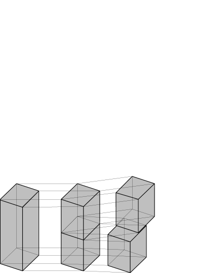
Figure 1: The spatio-temporal process of a volume object (left) splitting into two (middle) and one of them slipping away over time (middle to right) as a $4$-d space-time-complex.

3.1 Topological Extension of the Relational Model

What follows is a brief introduction into our topological data model BradleyPaul:DTop . Consider our aforementioned subdivision of space (or space-time) satisfying the following preconditions:

• A compact subset of the $n$-dimensional real space $\bbbr^{n}$ is subdivided into a finite number of parts.

• Each part is a connected $i$-dimensional manifold without boundary.

• Each such part is flat. That means it is within an $i$-dimensional affine subspace of $\bbbr^{n}$.

• The boundary of each $i$-dimensional part is the union of parts of lower dimensions.

We call this subdivision a finite polytope complex. Then the natural topology of the underlying $n$-dimensional real space $\bbbr^{n}$ generates a so-called quotient topology. As the number of parts is finite, their topology is finite, too, and, hence, it is a so-called Alexandrov-topology Alexandroff:Raeume which has an important characteristic: It can be stored by a relation called “incidence graph” and so it fits into a relational database:

Definition 1 (Topological Data Type)

Let $X$ be a set and $R\subseteq X\times X$ a relation on $X$. We call the pair $(X,R)$ a topological data type. A subset $A\subseteq X$ is said to be open in $(X,R)$, iff all $x\in X$ and $a\in A$ satisfy $x\,R\,a\Rightarrow x\in A$. The relation $R$ is also called the incidence relation of $(X,R)$.

So far we have only relabelled what is commonly known as simple directed graph. But note that every topology for a finite set can be stored in that simple manner.

Example 1 (Combinatorial Square)

We partition a unit square $[0,1]\times[0,1]$ $\subset\mathbb{R}^{2}$ into nine elements: four vertices $a=\left\{(0,1)\right\}$, $b=\left\{(1,1)\right\}$, $c=\left\{(0,0)\right\}$,and $d=\left\{(1,0)\right\}$, four edges $e={\left]0,1\right[}\times\left\{1\right\}$, $f=\left\{0\right\}\times{\left]0,1\right[}$, $g=\left\{1\right\}\times{\left]0,1\right[}$, and $h={\left]0,1\right[}\times\left\{0\right\}$, and the face $F={\left]0,1\right[}\times{\left]0,1\right[}$, which gives the topological space depicted at the left-hand side of the diagram below. At its right-hand side there is the corresponding topological datatype $(X,R)$ with point set $X=\left\{a,b,c,d,e,f,g,h,F\right\}$ and incidence relation

$$R=\left\{(x,y)\mid\text{The right image has an arrow $x\to y$.}\right\}.$$

The justification for relabelling “graph” to “topological data type” is our adaption of continuous maps to topological data types:

Definition 2 (Continuous Database Map)

Let $(X,R)$ and $(Y,S)$ be topological data types and $f:X\to Y$ a map. $S^{*}$ denotes the transitive and reflexive closure of $S$. We then call $f$ a continuous database map iff $(f(a),f(b))\in S^{*}$ holds for all $(a,b)\in R$. Then we write $f:(X,R)\to(Y,S)$.

The continuous database maps are exactly the continuous maps between the corresponding Alexandrov spaces. What we have in mind is a relational database table $X$ of spatial entities together with a table $R$ as an n:m relation type from $X$ to itself.

3.2 Algebraic Topology in Relational Databases

We now extend our above data model to algebraic topology: A Relational Chain Complex is a topological data type $(X,R)$ if the relation $R$ also carries additional information about the orientation of each cell by attaching signs to the cell-cell-incidences.

Here our partitioning of the space consists of a sequence $(C_{n},\ldots,C_{0})$ of sets $C_{i}$ of $i$-dimensional manifolds which together make up the entire space and which we call by abuse of language “$i$-cells”. Note that the above preconditions guarantee, that at least our $0$-“cells” and our $1$-“cells” are cells indeed. Each $i+1$-cell $c$ is orientable and bounded by a set $D$ of $i$-cells. By fixing an orientation for each cell in our partitioning we specify a sign for each cell $d$ in $D$ which depends on $c$: It is positive if $c$ is touched by $d$’s “front” side, negative at its “rear” side, or zero if $d$ touches $c$ by “both” sides. We refer to (Hatcher:AlgTop, , p. 233) for details on what “front” and “rear” in arbitrary dimension mean.

The above mentioned sign defines a function

$$\sigma_{c}:D\to\left\{-1,0,+1\right\};d\mapsto\begin{cases}+1&:\mbox{``front''}\\ \phantom{+}0&:\mbox{``both''}\\ -1&:\mbox{``rear''}\end{cases}\;.$$ (1)

Now we extend our relation $R$ from the topological data type $(X,R)$ to a function

$$M:R\to\bbbz,(x_{i+1},x_{i})\mapsto\sigma_{x_{i+i}}(x_{i})$$ (2)

and store it into a database table M with schema

$$\texttt{M(\text@underline{cell}:$X,$ \text@underline{boundar}y:$X,$ sigma:$\bbbz$)}.$$

Considering M a sparse matrix the matrix product of M with itself can be computed by

$$\begin{array}[]{ll}\lx@intercol\tt create~{}view~{}M\_squared~{}as\hfil\lx@intercol\\ \tt select&\tt~{}M1.cell,~{}M2.boundary,\\ &\tt~{}sum(M1.sigma*M2.sigma)~{}as~{}sigma\\ \tt from&\tt~{}M~{}M1,~{}M~{}M2\\ \tt where&\tt~{}M1.boundary=M2.cell\\ \tt group~{}by&\tt~{}M1.cell,~{}M2.boundary.\end{array}$$

If M_squared only contains zero entries it denotes a complex boundary. The above SQL-statement defines the multiplication of two sparse matrices M1 and M2 by simply replacing the from-clause by

$$\tt from~{}~{}M1,~{}M2.$$

Now we can define our data model:

Definition 3 (Relational Complex)

A sequence $(X_{n},\ldots,X_{0})$ of finite sets—the cells—together with a sequence $(D_{n},\ldots,D_{1})$ of sparse $X_{i}\times X_{i-1}$-matrices—the boundaries—is called a relational complex of dimension $n$ if every matrix product $D_{i+1}\cdot D_{i}$ of two consecutive matrices has only entries of value zero.

This definition fixes a static dimension upper bound $n$. Dynamic dimension is also possible: Collect all cells into a table $X$, all matrices into a table $D$, and specify dimension merely by an integer attribute. To specify geometry we simply store the $n$ coordinates of each vertex, say, in case $n=4$, by x, y, z, and t.

Example 2 (Combinatorial Square)

The following relational complex for Example 1 has Edges $e$ and $h$ running from left to right whereas Edges $f$ and $g$ point downwards. Face $F$ gets a counter-clockwise orientation:

The right-hand side shows the corresponding relational complex with point sets $X_{0}=\left\{a,b,c,d\right\}$, $X_{1}=\left\{e,f,g,h\right\}$, and $X_{2}=\left\{F\right\}$ and boundaries

$$R_{i}=\left\{(x,y,\pm 1)\mid x\in X_{i},y\in X_{i-1},\text{arrow $x\stackrel{{\scriptstyle\pm\,}}{{\longrightarrow}}y$ in right image below.}\right\}.$$

Note that the orientation of Edge $h$ is “compatible” with the orientation of Face $F$ so the entry in the boundary table is the tuple $(F,h,+1)$, whereas $g$ runs contrary to the face orientation as entry $(F,h,-1)$ indicates.

Now consider all paths from face $F$ to vertex $a$:

$$\lx@xy@svg{\hbox{\raise 0.0pt\hbox{\kern 4.90973pt\hbox{\ignorespaces\ignorespaces\ignorespaces\hbox{\vtop{\kern 0.0pt\offinterlineskip\halign{\entry@#!@&&\entry@@#!@\cr&&&&&&\crcr}}}\ignorespaces{\hbox{\kern-4.90973pt\raise 0.0pt\hbox{\hbox{\kern 0.0pt\raise 0.0pt\hbox{\hbox{\kern 1.0pt\raise 0.0pt\hbox{$\textstyle{F\ignorespaces\ignorespaces\ignorespaces\ignorespaces}$}}}}}}}\ignorespaces\ignorespaces\ignorespaces\ignorespaces{}{\hbox{\lx@xy@droprule}}\ignorespaces\ignorespaces\ignorespaces{\hbox{\kern 10.20227pt\raise 5.25555pt\hbox{{}\hbox{\kern 0.0pt\raise 0.0pt\hbox{\hbox{\kern 3.0pt\hbox{\hbox{\kern 0.0pt\raise-2.25555pt\hbox{$\scriptstyle{-1}$}}}\kern 3.0pt}}}}}}\ignorespaces{\hbox{\kern 28.90973pt\raise 0.0pt\hbox{\hbox{\kern 0.0pt\raise 0.0pt\hbox{\lx@xy@tip{1}\lx@xy@tip{-1}}}}}}{\hbox{\lx@xy@droprule}}{\hbox{\lx@xy@droprule}}{\hbox{\kern 28.90973pt\raise 0.0pt\hbox{\hbox{\kern 0.0pt\raise 0.0pt\hbox{\hbox{\kern 1.0pt\raise 0.0pt\hbox{$\textstyle{e\ignorespaces\ignorespaces\ignorespaces\ignorespaces}$}}}}}}}\ignorespaces\ignorespaces\ignorespaces\ignorespaces{}{\hbox{\lx@xy@droprule}}\ignorespaces\ignorespaces\ignorespaces{\hbox{\kern 41.80673pt\raise 5.25555pt\hbox{{}\hbox{\kern 0.0pt\raise 0.0pt\hbox{\hbox{\kern 3.0pt\hbox{\hbox{\kern 0.0pt\raise-2.25555pt\hbox{$\scriptstyle{-1}$}}}\kern 3.0pt}}}}}}\ignorespaces{\hbox{\kern 59.56598pt\raise 0.0pt\hbox{\hbox{\kern 0.0pt\raise 0.0pt\hbox{\lx@xy@tip{1}\lx@xy@tip{-1}}}}}}{\hbox{\lx@xy@droprule}}{\hbox{\lx@xy@droprule}}{\hbox{\kern 59.56598pt\raise 0.0pt\hbox{\hbox{\kern 0.0pt\raise 0.0pt\hbox{\hbox{\kern 1.0pt\raise 0.0pt\hbox{$\textstyle{a}$}}}}}}}{\hbox{\kern 90.85187pt\raise 0.0pt\hbox{\hbox{\kern 0.0pt\raise 0.0pt\hbox{\hbox{\kern 1.0pt\raise 0.0pt\hbox{$\textstyle{\text{and}}$}}}}}}}{\hbox{\kern 132.96301pt\raise 0.0pt\hbox{\hbox{\kern 0.0pt\raise 0.0pt\hbox{\hbox{\kern 1.0pt\raise 0.0pt\hbox{$\textstyle{F\ignorespaces\ignorespaces\ignorespaces\ignorespaces}$}}}}}}}\ignorespaces\ignorespaces\ignorespaces\ignorespaces{}{\hbox{\lx@xy@droprule}}\ignorespaces\ignorespaces\ignorespaces{\hbox{\kern 146.84843pt\raise 5.54723pt\hbox{{}\hbox{\kern 0.0pt\raise 0.0pt\hbox{\hbox{\kern 3.0pt\hbox{\hbox{\kern 0.0pt\raise-1.9639pt\hbox{$\scriptstyle{+1}$}}}\kern 3.0pt}}}}}}\ignorespaces{\hbox{\kern 166.78247pt\raise 0.0pt\hbox{\hbox{\kern 0.0pt\raise 0.0pt\hbox{\lx@xy@tip{1}\lx@xy@tip{-1}}}}}}{\hbox{\lx@xy@droprule}}{\hbox{\lx@xy@droprule}}{\hbox{\kern 166.78247pt\raise 0.0pt\hbox{\hbox{\kern 0.0pt\raise 0.0pt\hbox{\hbox{\kern 1.0pt\raise 0.0pt\hbox{$\textstyle{f\ignorespaces\ignorespaces\ignorespaces\ignorespaces}$}}}}}}}\ignorespaces\ignorespaces\ignorespaces\ignorespaces{}{\hbox{\lx@xy@droprule}}\ignorespaces\ignorespaces\ignorespaces{\hbox{\kern 180.66647pt\raise 5.25555pt\hbox{{}\hbox{\kern 0.0pt\raise 0.0pt\hbox{\hbox{\kern 3.0pt\hbox{\hbox{\kern 0.0pt\raise-2.25555pt\hbox{$\scriptstyle{-1}$}}}\kern 3.0pt}}}}}}\ignorespaces{\hbox{\kern 198.75473pt\raise 0.0pt\hbox{\hbox{\kern 0.0pt\raise 0.0pt\hbox{\lx@xy@tip{1}\lx@xy@tip{-1}}}}}}{\hbox{\lx@xy@droprule}}{\hbox{\lx@xy@droprule}}{\hbox{\kern 198.75473pt\raise 0.0pt\hbox{\hbox{\kern 0.0pt\raise 0.0pt\hbox{\hbox{\kern 1.0pt\raise 0.0pt\hbox{$\textstyle{a}$}}}}}}}\ignorespaces}}}}\ignorespaces. \textstyle{F\ignorespaces\ignorespaces\ignorespaces\ignorespaces} \scriptstyle{-1} \textstyle{e\ignorespaces\ignorespaces\ignorespaces\ignorespaces} \scriptstyle{-1} \textstyle{a} \textstyle{F\ignorespaces\ignorespaces\ignorespaces\ignorespaces} \scriptstyle{+1} \textstyle{f\ignorespaces\ignorespaces\ignorespaces\ignorespaces} \scriptstyle{-1} \textstyle{a} \textstyle{F\ignorespaces\ignorespaces\ignorespaces\ignorespaces} \scriptstyle{-1} \textstyle{e\ignorespaces\ignorespaces\ignorespaces\ignorespaces} \scriptstyle{-1} \textstyle{a} \textstyle{F\ignorespaces\ignorespaces\ignorespaces\ignorespaces} \scriptstyle{+1} \textstyle{f\ignorespaces\ignorespaces\ignorespaces\ignorespaces} \scriptstyle{-1} \textstyle{a}$$

When we multiply the coefficients of the first path we get $(-1)\times(-1)=+1$ and for the second path we have $(+1)\times(-1)=-1$. The sum of both is zero—the $F,a$-entry of the matrix product.

We also need a mapping between two relational complexes:

Definition 4 (Relational Complex Morphism)

Let $(X_{n},\ldots,X_{0})$ with boundaries $(D_{n},\ldots,D_{1})$ be a relational complex, and let $(Y_{n},\ldots,Y_{0})$ with boundaries $(B_{n},\ldots,B_{1})$ be another relational complex. Then we call a sequence $(F_{n},\ldots,F_{0})$ of (sparse) $X_{i}\times Y_{i}$-matrices a relational complex morphism, if each $D_{i}\cdot F_{i-1}=F_{i}\cdot B_{i}$ except for zero entries.

The above used difference $A-B$ of sparse matrices pads missing entries in one of the matrices with zero. From now on we say “algebraically equal” instead of “$a=b$ except for zero entries”.

4 Complex Overlay

Now having presented our data model we introduce the problem:

Two polytope complexes $C$ and $K$ partitioning a compact part $|C|$ and $|K|$ of the real vector space into flat manifolds have a common refinement of the intersection $|C|\cap|K|$: the polytope complex of $|C|\cap|K|$ of the non-empty pair-wise intersections of cells in $C$ and $K$. We call this intersection overlay and denote it by $C\cap K$.

Additionally there is a common refinement of $|C|\cup|K|$ which takes into account the exterior of the a complex if needed. This is union overlay, denoted by $C\cup K$.

Example 3 (Two Squares and a Triangle)

The union-overlay and intersection-overlay of a complex $S$ which consists of two meeting squares $ABDE$ and $BCEF$ with another complex $T$—simply the triangle $XYZ$—may be the following complexes $S\cup T$ (left) and $S\cap T$ (right):

The problem is: How can the intersection complex be computed?

5 Triangulation and Signed Decomposition

Triangulation is the partitioning of polygons into triangles which practically is in $O(n\log n)$, theoretically even in $O(n)$ Chazelle:Triangulation .

The $3$-d-analog is partitioning a polyhedron into tetrahedra and is often called “tetrahedralisation”. The worst case lower bound on the number of resulting tetrahedra is in $\Omega(n^{2})$, where $n$ is the number of cells Chazelle:ConvexPartitions .

The corresponding dimension-independent notion is “simplicial decomposition”. We know this is expensive but, happily, signed simplicial decomposition is often an alternative.

We will now present combinatorial $n$-d signed simplicial decompositions which generalise the well-known methods Boundary Triangulation BuelerEtAl:VolumeComputation , and Cohen Hickey’s Triangulation (CohenHickey:Triangulation , cited by BuelerEtAl:VolumeComputation ) by only using algebraic and topological information provided as relational complex.

5.1 Signed Boundary Decomposition

A signed decomposition of a cell $c$ into simplices $\pm\Delta_{1},\dotsc,\mp\Delta_{n}$ is a linear combination of simplices $\Delta_{1},\ldots,\Delta_{n}$ such that

$$c=\alpha_{1}\Delta_{1}+\cdots+\alpha_{n}\Delta_{n}$$ (3)

where $\alpha_{i}={+1}$ if the simplex is added and $\alpha_{i}={-1}$ if it is subtracted. As the order in which we add or subtract simplices does not matter one might also call this “Commutative Constructive Solid Geometry” (CCSG).

The algorithms presented here operate on the relational representation of a complex but we now take its “classical” view where each $C_{i}$ is the free Abelian group of cells in $X_{i}$, and the boundary operators $\partial_{i}$ are linear maps between them satisfying $\partial_{i-1}(\partial_{i}(x))=0$ for all $x\in C_{i}$. Now assume such complex

(4)

be given.

To triangulate an $n$-cell $c_{n}$ from $C_{n}$ (hence $c_{n}\in X_{n}$) we simply add an arbitrary point $a$ from the interior of $c_{n}$ as new vertex $a$ (“apex”) to the vertices and replace our cell $c_{n}$ by a “cone” $a\otimes\partial(c_{n})$ over its boundary with apex $a$. The tensor operator $a\otimes x$ is simply the concatenation of $a$ and $x$, either by creating a pair $(a,x)$ or by appending tuples:

$$a\otimes\partial(c_{n}) =a\otimes(\alpha_{1}\cdot d_{1}+\cdots+\alpha_{m}\cdot d_{m})$$

$$=a\otimes\alpha_{1}\cdot d_{1}+\cdots+a\otimes\alpha_{m}\cdot d_{m}$$ (5)

$$=\alpha_{1}\cdot a\otimes d_{1}+\cdots+\alpha_{m}\cdot a\otimes d_{m}$$

The boundary of one such such element $a\otimes d_{i}$ can be defined as

$$\partial(a\otimes d_{i}):=d_{i}-a\otimes\partial(d_{i}).$$ (6)

This is a boundary operator, indeed. It slightly modifies the Eilenberg-Zilber-formula EilenbergZilber:Product for tensor product boundaries

$$\delta(a\otimes x):=\delta(a)\otimes x+(-1)^{\dim a}a\otimes\delta(x)$$ (7)

to

$$\partial(a\otimes x):=\partial(a)\otimes x-(-1)^{\dim a}a\otimes\partial(x)$$ (8)

and specifies $\partial(a)=\langle\rangle$ which means that the boundary of the apex $a$ is the empty tuple—the identity element of concatenation: $\langle\rangle\otimes x=x=x\otimes\langle\rangle$. Subtraction instead of addition is achieved by simply “shifting” the dimension of $a$ from zero to 1 and considering $\langle\rangle$ having dimension 0.

In contrast to the original, our variant of the Eilenberg-Zilber-formula is compatible with the simplicial boundary operator which we denote here by $\delta$:

$$\partial (a\otimes\left\langle b,c,d,\ldots\right\rangle)$$

$$=\left\langle b,c,d,\ldots\right\rangle-\left\langle a,c,d,\ldots\right\rangle+\left\langle a,b,d,\ldots\right\rangle-\left\langle a,b,c,\ldots\right\rangle+\cdots$$

$$=\delta(\left\langle a,b,c,d,\ldots\right\rangle)$$ (9)

This even works for arbitrary $n$-simplices $\left\langle a_{0},\dotsc,a_{n}\right\rangle\otimes\left\langle b,c,d,\ldots\right\rangle$.

We remind that the simplicial boundary $\delta$ of a simplex $\left\langle v_{0},\dotsc,v_{n}\right\rangle$ is defined as

$$\delta(\left\langle v_{0},\dotsc,v_{n}\right\rangle):=\sum_{i=0}^{n}(-1)^{i}\left\langle v_{0},\dotsc,v_{i-1},\ v_{i+1},\dotsc,v_{n}\right\rangle.$$ (10)

Our “cone” over the boundary in fact has the same algebraic boundary as the original cell:

$$\partial(a\otimes\partial(c_{n})) =\partial(c_{n})-a\otimes\partial(\partial(c_{n}))=\partial(c_{n})-a\otimes 0$$

$$=\partial(c_{n}).$$ (11)

So a property of $c_{n}$ computed via its boundary can also be computed by the proposed triangulation—even when $a$ is outside $c_{n}$ or a vertex of the boundary of $c_{n}$.

Example 4 (Triangulating a Square)

The left hand side below shows a square $S$ in counter-clockwise orientation (as indicated by the bent arrow and the right hand side its triangulation with a newly introduced apex “$0$”:

The signs of the four triangles correspond to their orientation: If a triangle has clock-wise orientation (like $\left\langle 0,1,2\right\rangle$ which visits its vertices $0$, $1$, and $2$ in clock-wise order) it gets a negative sign. Each common edge of two adjacent signed triangles vanish when the boundary of their sum is computed. In $\partial(\left\langle 0,1,3\right\rangle-\left\langle 0,1,2\right\rangle)=+\left\langle 1,3\right\rangle-\left\langle 0,3\right\rangle+\left\langle 0,2\right\rangle-\left\langle 1,2\right\rangle+0\times\left\langle 0,1\right\rangle$, for example, the common edge $\left\langle 0,1\right\rangle$ cancels out.

The boundary of the left hand side complex is

$$\partial_{2}(S)=-\left\langle 1,2\right\rangle+\left\langle 1,3\right\rangle-\left\langle 2,4\right\rangle+\left\langle 3,4\right\rangle$$ (12)

for the face and

$$\partial_{1}(\left\langle 1,2\right\rangle) =\left\langle 2\right\rangle-\left\langle 1\right\rangle \partial_{1}(\left\langle 1,3\right\rangle) =\left\langle 3\right\rangle-\left\langle 1\right\rangle$$

$$\partial_{1}(\left\langle 2,4\right\rangle) =\left\langle 4\right\rangle-\left\langle 2\right\rangle \partial_{1}(\left\langle 3,4\right\rangle) =\left\langle 4\right\rangle-\left\langle 3\right\rangle$$ (13)

for the edges. The triangulation $\mu(S)$ then is:

$$\mu(S)="0"\otimes\partial_{2}(S) ="0"\otimes(-\left\langle 1,2\right\rangle+\left\langle 1,3\right\rangle-\left\langle 2,4\right\rangle+\left\langle 3,4\right\rangle)$$

$$=-\left\langle 0,1,2\right\rangle+\left\langle 0,1,3\right\rangle-\left\langle 0,2,4\right\rangle+\left\langle 0,3,4\right\rangle$$ (14)

Now, algebraically, $\mu(S)$ has the same boundary as $S$:

$$\partial(\mu(S)) =\partial(-\left\langle 0,1,2\right\rangle+\left\langle 0,1,3\right\rangle-\left\langle 0,2,4\right\rangle+\left\langle 0,3,4\right\rangle)$$

$$=-\partial\left\langle 0,1,2\right\rangle+\partial\left\langle 0,1,3\right\rangle-\partial\left\langle 0,2,4\right\rangle+\partial\left\langle 0,3,4\right\rangle)$$

$$=-(\left\langle 1,2\right\rangle-\left\langle 0,2\right\rangle+\left\langle 0,1\right\rangle)+(\left\langle 1,3\right\rangle-\left\langle 0,3\right\rangle+\left\langle 0,1\right\rangle)$$

$$\phantom{=\ }-(\left\langle 2,4\right\rangle-\left\langle 0,4\right\rangle+\left\langle 0,2\right\rangle)+(\left\langle 3,4\right\rangle-\left\langle 0,4\right\rangle+\left\langle 0,3\right\rangle)$$

$$=-\left\langle 1,2\right\rangle+\left\langle 1,3\right\rangle-\left\langle 2,4\right\rangle+\left\langle 3,4\right\rangle$$

$$=\partial_{2}(S).$$ (15)

Each summand $\pm\left\langle 0,x\right\rangle$ in the above sum where the simplex starts with $"0"$ has a simplex $\mp\left\langle 0,x\right\rangle$ such that both cancel to zero.

This approach, however, has a shortcoming: introducing a new vertex for each cell means that each sequence $(c_{n},c_{n-1},\dotsc,c_{0})$ of incident cells—a so-called cell tuple—is represented by one simplex. But this can result in extremely many simplices—the number of cell tuples then grows more than exponentially with the dimension of the complex. This is also true for our approach proposed next, but at least it greatly reduces the number of simplices.

Modifying Cohen and Hickey’s Approach

To ease the problem of the big number of simplices we use an existing boundary vertex instead of providing a new vertex for each cell. Then all boundary cells incident with that vertex degenerate, have a zero boundary, and can be dropped. We will now iteratively construct a signed simplicial decomposition as a morphism $\mu=(\mu_{n},\dotsc,\mu_{0})$ from our polytope complex $\mathcal{C}$ to a simplicial complex dimension by dimension starting with dimension zero, This morphism is then the desired signed simplicial decomposition.

We still denote the $i$-cells of our complex by $X_{i}$. At the first step the vertices $X_{0}$ in $C_{0}$ are simply labelled with integer numbers by $\mu_{0}$ which gives a bijection

$$\mu_{0}:X_{0}\to[1,\dotsc,\#X_{0}]\subseteq\bbbn$$ (16)

and its linear continuation to $C_{0}\to\bbbz[1,\dotsc,\#X_{0}]$. This specifies a linear order $<$ on the vertices and thereby a priori fixes an orientation of every simplex. The order is defined as $\ a<b:\Longleftrightarrow\mu_{0}(a)<\mu_{0}(b)\$ for all $a,b\in X_{0}$. We leave it open how permuting the labels can affect the size of the decomposition result and how we then can find an optimal $\mu_{0}$.

Each $i$-simplex is then an ascending sequence of $i+1$ different vertices. Our assumptions on the polytope imply that each edge $e\in X_{1}$ has two different boundary vertices $a$ and $b$ and one of them is the starting vertex and the other is the ending vertex. This gives two matrix entries $D_{1}(e,a)=-D_{1}(e,b)$ in the boundary matrix $D_{1}$. An entry $+1$ indicates an ending vertex and $-1$ stands for the starting vertex. This matrix entry of the maximal vertex will become the new sign of our image edge going from minimal to maximal vertex. Hence $\mu_{1}$ is defined by

$$\mu_{1}:X_{1}\to\bbbz[0,\dotsc,\#X_{0}]^{2},e\mapsto\begin{cases}D_{1}(e,b)\times\left\langle\mu_{0}(a),\mu_{0}(b)\right\rangle&:a<b\\ D_{1}(e,a)\times\left\langle\mu_{0}(b),\mu_{0}(a)\right\rangle&:b<a\;.\end{cases}$$ (17)

This function inverts the edge orientation and the sign when its vertices are ordered against their total ordering imposed by $\mu_{0}$ and guarantees that the first vertex in the simplex $\left\langle a,b\right\rangle$ is always minimal. Note that the first two vertices are always different. Now this guarantee will be kept throughout every dimension. Here we denote the $i^{\text{th}}$ simplicial boundary by $\delta_{i}$.

We now show that our partially finished signed decomposition $(\mu_{1},\mu_{0})$ is a morphism from the $1$-skeleton $(X_{1},X_{0})$ to a simplicial complex $\Delta$ by showing

$$\delta_{1}\circ\mu_{1}=\mu_{0}\circ\partial_{1}\;.$$ (18)

Let $e$ be an edge in $X_{1}$, $a$ its starting vertex, and $b$ be the ending vertex. This means $\partial_{1}(e)=b-a$. and $D_{1}(e,b)={+1}$ and $D_{1}(e,a)={-1}$. Then for the right hand side of Equation (18) we have:

$$\mu_{0}(\partial_{1}(e)) =\mu_{0}(b-a)=\mu_{0}(b)-\mu_{0}(a)$$ (19)

In case $$a<b$$ we have for the left-hand side:

$$\delta_{1}(\mu_{1}(e)) =\delta_{1}(D_{1}(e,b)\times\left\langle\mu_{0}(a),\mu_{0}(b)\right\rangle)=\delta_{1}\left\langle\mu_{0}(a),\mu_{0}(b)\right\rangle$$

$$=\mu_{0}(b)-\mu_{0}(a)\;.$$ (20)

In case $$b<a$$ the left hand side gives:

$$\delta_{1}(\mu_{1}(e)) =\delta_{1}(D_{1}(e,a)\times\left\langle\mu_{0}(b),\mu_{0}(a)\right\rangle)=\delta_{1}(-\left\langle\mu_{0}(b),\mu_{0}(a)\right\rangle)$$

$$=-\delta_{1}(\left\langle\mu_{0}(b),\mu_{0}(a)\right\rangle)=-(\mu_{0}(a)-\mu_{0}(b))$$

$$=\mu_{0}(b)-\mu_{0}(a)\;.$$ (21)

In both cases we have $\mu_{0}(\partial_{1}(e))=\delta_{1}(\mu_{1}(e))$ for every edge $e$ and therefore Equation (18) holds.

The higher dimensional maps $\mu_{2},\mu_{3},\ldots$ can now be computed iteratively each of them using its previously accomplished predecessor: Let $\mu_{i}$ be given. Then we use it to compute $\mu_{i+1}$ from $\mu_{i}$ and $\partial_{i+1}$ for each $i+1$-cell $c$ in $C_{i+1}$: First take the given boundary $\partial_{i+1}(c)$ which is a linear combination

$$\partial_{i+1}(c)=\alpha_{1}d_{1}+\dotsb+\alpha_{k}d_{k}$$ (22)

where the $\alpha_{j}$ are the entries $D_{i+1}(c,d_{j})$ in the boundary matrix $D_{i+1}$ of $\partial_{i+1}$. Then compute the image of $\partial_{i+1}(c)$ under the morphism $\mu_{i}$ which gives

$$\mu_{i}\circ\partial_{i+1}(c)=\alpha_{1}\mu_{i}(d_{1})+\dotsb+\alpha_{k}\mu_{i}(d_{k}).$$ (23)

We know that each simplex $\mu_{i}(d_{j})$ in above Equation (23) is a sequence $\left\langle\nu_{0},\dotsc,\nu_{i}\right\rangle$ of vertex numbers (given by $\mu_{0}$) in strictly ascending order. Therefore the first vertex number $\nu_{0}$ is minimal in that simplex. We now take the minimal number $a$ of all these vertices in the boundary of $c$ and define

$$a\otimes\mu_{i}\circ\partial_{i+1}(c)=\alpha_{1}\times a\otimes\mu_{i}(d_{1})+\dotsb+\alpha_{k}\times a\otimes\mu_{i}(d_{k})$$ (24)

which is a linear combination of simplices $\left\langle a,\nu_{0},\dotsc,\nu_{i}\right\rangle$ which are the $i$-simplices of the triangulated boundary of $c$ with the minimal vertex $a$ attached at front to get a new $i+1$ simplex.

The operator $a\otimes\mu_{i}\circ\partial_{i+1}$, in fact, is a morphism:

$$\delta_{i+1} (a\otimes\mu_{i}\circ\partial_{i+1}(c))$$

$$=\mu_{i}\circ\partial_{i+1}(c)-a\otimes\delta_{i}(\mu_{i}\circ\partial_{i+1}(c))$$  by Eqn. (6)

$$=\mu_{i}\circ\partial_{i+1}(c)-a\otimes\delta_{i}\circ\mu_{i}\circ\partial_{i+1}(c)$$

$$=\mu_{i}\circ\partial_{i+1}(c)-a\otimes\mu_{i-1}(\partial_{i}\circ\partial_{i+1}(c)) \mu_{i}$$  by being a morphism

$$=\mu_{i}\circ\partial_{i+1}(c)-a\otimes\mu_{i-1}\circ\hat{0}(c) \partial$$  by being a boundary

$$=\mu_{i}\circ\partial_{i+1}(c)-a\otimes 0$$

$$=\mu_{i}\circ\partial_{i+1}(c).$$ (25)

Now each boundary simplex $\left\langle\nu_{1},\dotsc,\nu_{n}\right\rangle$ which contains $a$ has that vertex $a$ at its front because it is the minimal vertex of all boundary simplices and $\nu_{1}$ is the minimal vertex of that simplex. Hence $a=\nu_{1}$ and thus the simplex degenerates to $\left\langle a,a,\nu_{2},\dotsc,\nu_{n}\right\rangle$. But then every non-zero summand of its simplicial boundary also starts with $\left\langle a,a,\dotsc\right\rangle$.

But such an element does not occur in $\delta_{i}\circ\mu_{i-1}(c)$ because all vertices in all simplices in $\mu_{i-1}(c)$ are different by precondition. By the morphism property $\delta_{i}\circ\mu_{i-1}(c)=\mu_{i}\circ\partial_{i+1}(c)$ these elements can occur in $\mu_{i}\circ\partial_{i+1}(c)$ only with a zero coefficient and therefore can be removed from $\mu_{i}\circ\partial_{i+1}(c)$ without (algebraically) modifying the boundary $\delta_{i+1}$.

Our new morphism $\mu_{i+1}$ does exactly this and thus guarantees the precondition that all vertices of a simplex are different:

$$\mu_{i+1}(c):=a_{c}\otimes\mu^{(a_{c})}_{i}\circ\partial_{i+1}(c)$$ (26)

where $a_{c}$ is the minimal vertex touching $c$ and $\mu^{(a_{c})}_{i}$ is $\mu_{i}$ after having removed all simplices containing $a_{c}$.

Example 5 (Triangulating our Square Again)

The left hand side diagram shows a square $S$ and the right hand side its triangulation. We do this step by step starting with $\mu_{0}$ which enumerates the vertices in an arbitrary manner:

Now we can compute the edges which run from lower to higher vertex number:

Remember, the the boundary of $S$ is $\partial_{2}(S)=cd-bd-ab+ac$. Then

$$\mu_{1}(\partial_{2}(S)) =\mu_{1}(cd)-\mu_{1}(bd)-\mu_{1}(ab)+\mu_{1}(ac)$$

$$=\left\langle 1,3\right\rangle-\left\langle 2,3\right\rangle-(-\left\langle 2,4\right\rangle)+(-\left\langle 1,4\right\rangle)$$

$$=\left\langle 1,3\right\rangle-\left\langle 2,3\right\rangle+\left\langle 2,4\right\rangle-\left\langle 1,4\right\rangle$$ (27)

We take the minimal vertex $$1 1 1$$, remove all simplices that start with , and then append to the remaining simplices:

$$\mu_{2}(S) =-\left\langle 1,2,3\right\rangle+\left\langle 1,2,4\right\rangle$$ (28)

Note that the $2$-simplex (or triangle) $\left\langle 1,2,4\right\rangle$ is oriented counter-clockwise just as the face $S$ and therefore gets a positive sign whereas triangle $\left\langle 1,2,3\right\rangle$ is oriented clockwise and accordingly gets a negative sign to indicate that is must be flipped to be compatible with the orientation of $S$.

Finally the simplices, which are still tuples $\left\langle\nu_{0},\dotsc,\nu_{i}\right\rangle$ of natural numbers are considered simplices in $\bbbr^{n}$ by application of $\mu_{0}^{-1}$, the inverse of $\mu_{0}$. This gives $\left\langle v_{0},\dotsc,v_{i}\right\rangle=\left\langle\mu_{0}^{-1}(\nu_{0}),\dotsc,\mu_{0}^{-1}(\nu_{i})\right\rangle$.

Now the $n$-d “commutative CSG” is defined as follows: If the sign of the $n$-simplex orientation matches the sign assigned to it by the morphism the (absolute) simplex volume will be added to the polytope cell whereas in case that orientation sign and assigned sign are different the (absolute) simplex volume will be removed from the polytope. “Simplex orientation” of an $n$-simplex in $\bbbr^{n}$ can easily be computed: The determinant

$$\det(\left\langle v_{0},\dotsc,v_{n}\right\rangle)=\left|\ \begin{array}[]{c@{\quad}c@{\quad}c@{\quad}c}x_{1}-x_{0}&x_{2}-x_{0}&\cdots&x_{n}-x_{0}\\ y_{1}-y_{0}&y_{2}-y_{0}&\cdots&y_{n}-y_{0}\\ \vdots&\vdots&\ddots&\vdots\\ z_{1}-z_{0}&z_{2}-z_{0}&\cdots&z_{n}-z_{0}\end{array}\ \right|$$ (29)

has $n!$ times the signed volume of the corresponding simplex and the sign is the orientation. The values $x_{i},y_{i},\ldots,z_{i}$ are the $n$ vertex coordinates of vertex $v_{i}$.

6 Simplex Intersection

One application of such signed decomposition is polytope intersection or—more generally—polytope complex intersection: the pair-wise intersection of cells in a polytope complex which itself gives a new polytope complex.

Wit those signed simplices $\mu$ we compute the polytope complex intersection of, say, $\mathcal{C}$ and $\mathcal{K}$. But how do we intersect simplices?

6.1 Application of the Active-Set-Method

Assume there are two simplices: an $n$-simplex $a=\left\langle a_{0},\ldots,a_{n}\right\rangle$ and an $m$-simplex $b=\left\langle b_{0},\ldots,b_{m}\right\rangle$. We will give a brief sketch of how the cells of the intersection complex of $a\cap b$ can be found using a modified version of the active-set-method Nocedal:Optimization a well-known numerical optimisation technique.

Each point $p$ in a simplex $\left\langle a_{0},\dotsc,a_{n}\right\rangle$ has convex coordinates $(\alpha_{0},$ $\dotsc,\alpha_{n})$ such that $p=\alpha_{0}a_{0}+\dotsb+\alpha_{n}a_{n}$. In other words, these coordinates must sum up to $1$ and neither is negative. Let $q=\beta_{0}b_{0}+\dotsb+\beta_{m}b_{m}$ be such point in the other simplex $b$. Then the pair of points $(p,q)$ can be expressed by concatenating their barycentric coordinates to a vector $\vec{x}=(\alpha_{0},\dotsc\alpha_{n},\,\beta_{0},\dotsc,\beta_{m})$. It represents an intersection iff (the square of) the distance of $p$ and $q$ is zero. The square of the distance can be computed by inserting $\vec{x}$ into

$$d^{2}(\vec{x})=\vec{x}\cdot\left(\begin{array}[]{cccccccccccccccccc}a_{0}a_{0}&\cdots&a_{0}a_{n}&&-a_{0}b_{0}&\cdots&-a_{0}b_{m}\\ \vdots&\ddots&\vdots&&\vdots&\ddots&\vdots\\ a_{n}a_{0}&\cdots&a_{n}a_{n}&&-a_{n}b_{0}&\cdots&-a_{n}b_{m}\\[3.0pt] -b_{0}a_{0}&\cdots&-b_{0}a_{n}&&b_{0}b_{0}&\cdots&b_{0}b_{m}\\ \vdots&\ddots&\vdots&&\vdots&\ddots&\vdots\\ -b_{m}a_{0}&\cdots&-b_{m}a_{n}&&b_{m}b_{0}&\cdots&b_{m}b_{m}\end{array}\right)\cdot\vec{x}^{T}$$ (30)

a so-called “quadratic form”. The matrix entries are the dot product of the vertices in $\bbbr^{n}$. To minimise this equation, subject to the constraints

$$\alpha_{0}+\dotsb+\alpha_{n}\ ={\quad 1\quad}=\ \beta_{0}+\dotsb+\beta_{m},$$ (31)

the following Karush-Kuhn-Tucker-system (or KKT-system) must be solved:

$$\left(\begin{array}[]{cccccccccccccccccc}a_{0}a_{0}&\cdots&a_{0}a_{n}&-a_{0}b_{0}&\cdots&-a_{0}b_{m}&1&&0\\ \vdots&\ddots&\vdots&\vdots&\ddots&\vdots&\vdots&&\vdots\\ a_{n}a_{0}&\cdots&a_{n}a_{n}&-a_{n}b_{0}&\cdots&-a_{n}b_{m}&1&&0\\[3.0pt] -b_{0}a_{0}&\cdots&-b_{0}a_{n}&b_{0}b_{0}&\cdots&b_{0}b_{m}&0&&1\\ \vdots&\ddots&\vdots&\vdots&\ddots&\vdots&\vdots&&\vdots\\ -b_{m}a_{0}&\cdots&-b_{m}a_{n}&b_{m}b_{0}&\cdots&b_{m}b_{m}&0&&1\\[3.0pt] 1&\cdots&1&0&\cdots&0&0&&0\\ 0&\cdots&0&1&\cdots&1&0&&0\\ \end{array}\right)\cdot\left(\begin{array}[]{cccccccccccccccccc}\alpha_{0}\\ \vdots\\ \alpha_{n}\\[3.0pt] \beta_{0}\\ \vdots\\ \beta_{m}\\[3.0pt] \Lambda_{a}\\ \Lambda_{b}\\ \end{array}\right)=\left(\begin{array}[]{cccccccccccccccccc}0\\ \vdots\\ 0\\[3.0pt] 0\\ \vdots\\ 0\\[3.0pt] 1\\ 1\\ \end{array}\right)$$ (32)

Note that the last two lines of this equation system are Equations (31).

Now a vertex is called active at $\vec{x}$ if its corresponding barycentric coordinate is zero, and otherwise inactive. A vector is feasible iff it represents a convex combination of the vertices, hence iff none of the barycentric coordinates is negative. A set of vertices is feasible if its KKT-system has a unique feasible solution.

To find all intersection cells of the two simplices we first compute the intersection vertices with the following algorithm:

• Initialise a set $S=\left\{\left\{a_{i},b_{j}\right\}\mid i=0\dotsc n,j=0\dotsc m\right\}$, the initially inactive sets, and initialise an empty set $R$ (the “Result”).

• While $S$ is not empty do:

  • Chose one inactive set $I$ from $S$ and remove it from $S$.

  • Restrict the KKT-system of Equation (32) to $I$ and solve it, say, by calling LAPACK’s dgesv-routine LAPACK:UGuide . “Restrict” means “remove each row and column $x$ which is not in $I$ from the equation system” (or, equivalently, set each such row and column $x$ in the matrix to $0$ and then the diagonal entry at $x$ to $1$).

  • If the solution is unfeasible the intersection point is outside of one of the simplices. Then discard $I$ and continue the loop with the next $I$ from $S$.

  • Otherwise, if the Lagrangian multipliers $\Lambda_{a}$ and $\Lambda_{b}$ of the solution are both zero, the corresponding simplices intersect at the point with these barycentric coordinates. Then add $I$ to $R$, because $I$ then indicates an intersection vertex of the simplex intersection.

  • If the solution is feasible but at least one of the Lagrangians is not zero the simplices are either skew or parallel and their affine spaces do not intersect. Then multiply the solution with the Matrix of the unrestricted KKT-system. This gives (half) the gradient of the (squared) distance function at $\vec{x}$. Then for each vertex $v_{i}\notin I$ where that gradient is negative add $I+\left\{v_{i}\right\}$ to $S$.

• When $S$ is empty return result $R$.

We can prove that this algorithm always terminates and computes every minimal inactive set for each vertex of the simplex intersection. We will not carry out that proof here. It consists in showing that every such inactive set has a sequence of vertices which can be removed one by one without rendering the remaining set unfeasible until it becomes one of the initially inactive sets.

A forthcoming paper will show how we handle ill-conditioned matrices and “critical” intersections like an intersection of a vertex with an edge of a triangle.

Each set $I$ in the above computed set $R$ is a set of vertices denoting a pair of sides one from each simplex. This pair of sides intersects in one unique point. To get the higher-dimensional intersection cells we simply compute all possible unions of these inactive sets.

The following diagram shows an intersection of two triangles on the left hand side together with the inactive sets of the intersection vertices on the right-hand side:

The vertex $\left\{1,3,4,6\right\}$ indicates that it is on the intersection of edge $\left\langle 1,3\right\rangle$ with edge $\left\langle 4,6\right\rangle$, whereas $\left\{1,2,3,6\right\}$ denotes the intersection of vertex $6$ with triangle $\left\langle 1,2,3\right\rangle$. Note that $\left\{1,3,4,5\right\}\cup\left\{2,3,4,5\right\}=\left\{1,2,3,4,5\right\}$—the union of the inactive sets of the two bottom vertices—gives the inactive set of the bottom line between these vertices. If we restrict the KKT-system to that set then its solution space is of dimension one. It contains the barycentric coordinates of all points in the affine space of that edge, whereas the feasible solutions denote the points on that edge itself.

6.2 The Algebraic Simplex Intersection Boundary

From now on we will write the sets $\left\{1,2,3,5\right\}$ as $"1235"$, i.e. a string of integers. What follows is the set of all unions of $"1345"$, $"2345"$, $"1346"$, $"2356"$, and $"1236"$:

$$X=\{ "1345","2345","1346","2356","1236",$$ the vertices

$$"12345","13456","23456","12346","12356",$$ the edges (33)

$$"123456"\}$$ the face

This gives a topological data type $(X,\supseteq)$ where each set is bounded by its subsets in $X$. To get a relational complex we need an algebraic boundary operator. A possible solution could be to restrict the simplicial boundary to $X$. This gives indeed a complex boundary (see also Lefschetz:ComplexIntersection ) but none which is useful for our purpose. We will indicate restriction to $X$ by either ${<}\text{expr}{>}|_{X}$ or by striking out sets which are not in $X$. Let us try that simple approach: Computing some edge boundary gives strange edges like

$$\partial|_{X}("23456") =+\text{"\sout{3456}"}-\text{"\sout{2456}"}+"2356"-\text{"\sout{2346}"}+"2345"$$

$$=+"2356"+"2345".$$ (34)

Remember that a positive sign indicates “end point”, and a negative sign is attached to a starting point. So we see that, instead of assigning a starting point and an endpoint, that boundary operator assigns two endpoints “2356” and “2345” and no starting point to the edge “23456”. Hence, that boundary defines no orientation. Computing the boundary of the face and all edges gives the following result:

On the right hand side we have inverted the edges with a negative face-edge-incidence to illustrate the edges cycle. This strange boundary does not define an orientation of the face—one part of the boundary surrounds the face in counter-clock-wise direction whereas the other part goes clock-wise. Both these parts start with a common edge that has two endpoints and end with another common edge with two starting points (upper left). Anyway, formally this is a valid cycle and the result, in fact, constitutes a complex. We suppose that we can take that boundary as it is for our next algorithmic step.

As we might need an orientation for that step, however, we came up so far with an algorithm which iterates the dimensions starting with $1$ (the edges) and attaches an arbitrary orientation to each cell. Because of the manifold property of each cell we can specify an orientation of $c$ by merely attaching one arbitrary sign, say $+1$, to a cell-incidence $R(c,d)$ from $c$ to an already oriented boundary cell $d$. This sign then determines the signs of all other incidences of that cell $c$ with its boundary cells.

Finally the orientation of the $n$-cells may have to be inverted, because later we want that the orientation of each resulting $n$-cell is the product of the orientations of the intersecting $n$-simplices. By now this restricts the validity of the next algorithmic step to full-dimensional complexes, in other words, it might only work with $n$-d complexes in $\bbbr^{n}$.

7 Summing Simplex Intersections

We simply sum up all these intersection complexes thereby respecting the previously attached signs to get the resulting intersection complex. If the intersected simplices have different signs then the intersection complex will be subtracted from the resulting complex and otherwise added. Then the simplex boundary cells that have been introduced by the triangulation will cancel to zero. We will show that this at least works with full-dimensional complexes:

Let $p$ be a point in $\bbbr^{n}$ and let $\sigma=\left\langle v_{0},\dotsc,v_{n}\right\rangle$ be an $n$-simplex in $\bbbr^{n}$. Then $p$ is almost never a boundary point and, hence, can be considered either an interior or an exterior point. If $p$ is an interior point, the boundary “wraps around” $p$ one or several times in some “direction”. This is called the degree (or winding number) of $\sigma$’s boundary with respect to $p$ and is nothing but the orientation of $\sigma$ which is non-zero. If $p$ is an exterior point, however, we have winding number $0$.

But the winding number of a cell’s boundary $\partial(c)$ is the same as the sum of the signed winding numbers of the simplices’ boundaries in the signed decomposition of $c$. This is also true for another triangulated $n$-cell $z$ of the other complex. Let us denote the winding number of a cell boundary $\partial(c)$ at point $p$ by $w(p,c)$. Then for the decomposition $\mu_{n}(c)=\alpha_{1}\sigma_{1}+\dotsb+\alpha_{k}\sigma_{k}$ into simplices $\sigma_{i}$ we have

$$w(p,c)=\alpha_{1}w(p,\sigma_{1})+\dotsb+\alpha_{k}w(p,\sigma_{k}).$$ (35)

Now $p$ is an interior point of $c\cap z$ iff both winding numbers are non-zero, or, equivalently, iff the product of both winding numbers is non-zero. Then we have

$$p\in c\cap z\Leftrightarrow w(p,c)\cdot w(p,z)\neq 0$$ (36)

As we have a boundary for a simplex intersection $\sigma_{a}\cap\sigma_{b}$ such that $w(p,\sigma_{a})\cdot w(p,\sigma_{b})=w(p,\sigma_{a}\cap\sigma_{b})$ we can compute $w(p,c)\cdot w(p,z)$ by

$$w(p,c)\cdot w(p,z) =(\alpha_{1}w(p,\sigma_{1})+\dotsb+\alpha_{n}w(p,\sigma_{i}))\cdot$$

$$\phantom{{}={}}(\beta_{1}w(p,\zeta_{1})+\dotsb+\beta_{m}w(p,\zeta_{m}))$$

$$=\sum_{i=1}^{n}\sum_{j=1}^{m}\alpha_{i}\beta_{j}w(p,\sigma_{i}\cap\zeta_{j})$$ (37)

As $w(p,\emptyset)=0$ we only have to sum up the winding numbers of non-empty simplex intersections with coefficients $\alpha_{i}\beta_{j}$. This is the reason for our above mentioned restriction on the orientation of the simplex intersection. Of course, here spatial indexing or a sweeping hyperplane approach would increase efficiency, but we will not particularise spatial indexing here.

Then the refinement that stems from the signed decomposition must be undone. Therefore the simplex-simplex intersections will be re-composed to get the final result by using the inverse of the two morphisms $\mu_{\mathcal{C}}$ and $\mu_{\mathcal{K}}$.

Finally, as intersecting possibly non-convex cells may give non-connected resulting cells, it is also possible—but not necessary—to identify connected components of cell intersections if this is needed.

8 Applications and Outlook

Polytope complex intersection can be used to compute “topological relations”, to overlay spatial structures like a geological formation and a drilling path or the “common footprint” of two geological structures that meet at a fault. It can also be used to combine spatial data sets, say, a city model and a GIS data set, into one. It is dimension independent and, for example, can also be applied to cut temporal slices out of a 4D space-time complex.

So we have shown a relational database schema for polytope complexes of any dimension and an intersection algorithm for full-dimensional complexes which seems efficient.

However, even if this combinatorial decomposition looks quite efficient there is a general complexity problem: If we combinatorially triangulate an $n$-dimensional hypercube we get $n!$ simplices. So the number of simplices can grow super-exponentially with the complexity of the triangulated polytope if there is no fixed dimension upper bound. In practice dimension might be bounded from above by $5$: E.g. three spatial dimensions, time, and, maybe, version history. Then our triangulation creates $5!=120$ simplices for a cube. In future we therefore want to study polytope complex overlay by using a signed convex cell decomposition into more general convex shapes. However, we suspect that the above mentioned complexity explosion with unbounded dimension is fundamental, yet another curse of dimensionality, and cannot be overcome by any algorithm be it smarter than the one presented here or not.

Additionally, it is worthwhile to further investigate the strange results of “purely algebraic” boundary operators. First it should be investigated if such strange boundary could simply be tolerated when intersections are summed up. One could also search for an alternative to compute intersected cell orientation more deterministically than choosing an arbitrary initial “seed” incidence sign. In particular all this should lead to intersect complexes of different dimension or of lower dimension than the embedding space.

Also, the algorithm computes many simplex-simplex-intersections which later disappear at the re-composition phase and, hence, need not be computed. So it might save computation time if these intersections were identified in advance and not computed at all.

References

- (1) Alexandroff, P.: Diskrete Räume. Matematiećeskij Sbornik 44(2), 501–519 (1937). URL http://mi.mathnet.ru/msb5579
- (2) Anderson, E. (ed.): LAPACK users guide, 3. ed. edn. Software environments tools. Society for Industrial and Applied Mathematics, Philadelphia, Pa. (1999). URL http://www.netlib.org/lapack/lug/
- (3) Bradley, P.E., Paul, N.: Using the Relational Model to Capture Topological Information of Spaces. The Computer Journal 53(1), 69–89 (2010). DOI 10.1093/comjnl/bxn054
- (4) Büeler, B., Enge, A., Fukuda, K.: Polytopes - Combinatorics and Computation, chap. Exact volume computation for convex polytopes: A practical study. Birkhäuser (2000)
- (5) Bulbul, R., Frank, A.: AHD: The alternate hierarchical decomposition of nonconvex polytopes. In: Geoinformatics, 2009 17th International Conference on, pp. 1–6 (2009). DOI 10.1109/GEOINFORMATICS.2009.5293499
- (6) Bulbul, R., Karimipour, F., Frank, A.U.: A simplex based dimension independent approach for convex decomposition of nonconvex polytopes. In: B.G. Lees, S.W. Laffan (eds.) 10th International Conference on GeoComputation. UNSW, Sydney (2009)
- (7) Chazelle, B.: Convex partitions of polyhedra: A lower bound and worst-case optimal algorithm. SIAM Journal on Computing pp. 488–507 vol.13 no.3 (1984)
- (8) Chazelle, B.: Triangulating a simple polygon in linear time. Discrete and Computational Geometry pp. 485–524 vol.6 (1991)
- (9) Chazelle, B., Palios, L.: Decomposition algorithms in geometry. In: C. Bajaj (ed.) Algebraic Geometry and its Applications, chap. 27, pp. 419–447. Springer-Verlag (1994)
- (10) Cohen, J., Hickey, T.: Two algorithms for determining volumes of convex polyhedra. Journal of the ACM 26(3), 401–414 (1979)
- (11) Eilenberg, S., Zilber, J.A.: On products of complexes. American Journal of Mathematics 75(1), 200–204 (1953)
- (12) Hatcher, A.: Algebraic Topology. Cambridge University Press (2002). URL http://www.math.cornell.edu/~hatcher/
- (13) Khachiyan, L., Boros, E., Borys, K., Elbassioni, K., Gurvich, V.: Generating all vertices of a polyhedron is hard. Discrete Comput Geom 39, 174–190 (2008). DOI 10.1007/s00454-008-9050-5
- (14) Lawrence, J.: Ppolytope volume computation. Mathematics of Computation 57(195), 174–190 (1991)
- (15) Lefschetz, S.: Intersections and transformations of complexes and manifolds. Transactions of the American Mathematical Society 28(1), 1–49 (1926). URL http://www.jstor.org/stable/1989171
- (16) Nocedal, J., Wright, S.J.: Numerical optimization, 2. ed. edn. Springer series in operation research and financial engineering. Springer, New York, NY (2006)
- (17) Streilein, A.: 3d data management — relevance for a 3d cadastre, position paper 3. 2nd International Workshop on 3D Cadastres (2011)