Frequency-dependent streaming potentials: a review

Abstract

This paper has been published in: International J. of Geophysics, vol 2012, article ID 648781, doi:10.1155/2012/648781
open access at: www.hindawi.com/journals/ijgp/2012/648781

The interpretation of seismoelectric observations involves the dynamic electrokinetic coupling, which is related to the streaming potential coefficient. We describe the different models of the frequency-dependent streaming potential, mainly the Packard’s and the Pride’s model. We compare the transition frequency separating low-frequency viscous flow and high-frequency inertial flow, for dynamic permeability and dynamic streaming potential. We show that the transition frequency, on a various collection of samples for which both formation factor and permeability are measured, is predicted to depend on the permeability as inversely proportional to the permeability. We review the experimental setups built to be able to perform dynamic measurements. And we present some measurements and calculations of the dynamic streaming potential.

1 Introduction

Electrokinetics arise from the interaction between the rock matrix and the pore water. Therefore electrokinetic phenomena are often observed in aquifers, volcanoes, and hydrocarbon or hydrothermal reservoirs. Observations show that seismoelectromagnetic signals associated to earthquakes can be induced by electromagnetic induction (Honkura et al., 2009; Matsushima et al., 2002) or by electrokinetic effect (Takeuchi et al., 1998; Fenoglio et al., 1995). The electrokinetic phenomena are due to pore pressure gradients leading to fluid flow in the porous media or fractures, and inducing electrical fields. These electrokinetic effects are associated to the electrical double layer which was originally described by Stern. The electrokinetic signals can be induced by global displacements of the reservoir fluids (streaming potential) or by the propagation of seismic waves (seismoelectromagnetic effect). As soon as these pressure gradients have a transient signature, the dynamic part of the electrokinetic coupling has to be taken into account by introducing the dependence on fluid transport properties.

It is generally admitted that two kinds of seismoelectromagnetic effects can be observed. The dominant contribution, commonly called “coseismic”, is generated close to the receivers during the passage of seismic waves. The second kind, so called “interfacial conversion”(Dupuis et al., 2009), is very similar to dipole radiation and is generated at physico-chemical interfaces due to strong electrokinetic coupling discontinuities. This interface conversion is often perceived to have the potential to detect fine fluids transitions with higher resolution than seismic investigations, but in practice, signals are often masked by electromagnetic disturbances, especially when generated at great depth.

Nevertheless recent field studies have focused on the seismo-electric conversions linked to electrokinetics in order to investigate oil and gas reservoirs (Thompson et al., 2005) or hydraulic reservoirs (Dupuis & Butler, 2006; Dupuis et al., 2007, 2009; Strahser et al., 2007; Haines et al., 2007a, b; Strahser et al., 2011; Garambois & Dietrich, 2001). It has been shown using these investigations that not only the depth of the reservoir can be deduced, but also the geometry of the reservoir can be imaged using the amplitudes of the electro-seismic signals (Thompson et al., 2007). Moreover fractured zones can be detected and permeability can be measured using seismo-electrics in borehole (Singer et al., 2005; Pain et al., 2005; Mikhailov et al., 2000; Jouniaux, 2011). This method is especially appealing to hydrogeophysics for the detection of subsurface interfaces induced by contrasts in permeability, in porosity, or in electrical properties (salinity and water content) (Schakel et al., 2011; Schakel & Smeulders, 2010; Garambois & Dietrich, 2002).

The analytical interpretation of the seismoelectromagnetic phenomenon has been described by Pride (1994), by connecting the theory of Biot (1956) for the seismic wave propagation in a two phases medium with Maxwell’s equations, using dynamic electrokinetic couplings. The seismoelectromagnetic conversions have been modeled in homogeneous or layered saturated media (Haartsen & Pride, 1997; Haartsen et al., 1998; Garambois & Dietrich, 2001, 2002; Gao & Hu, 2010) with applications to reservoir geophysics (Saunders et al., 2006).

Theoretical developments showed that the electrical field induced by the $P$-waves propagation is related to the acceleration (Garambois & Dietrich, 2001). The electrokinetic coupling is created at the interface between grains and water, when there is a relative motion of electrolyte ions with respect to the mineral surface. Thus, seismic wave propagation in fluid-filled porous media generates conversions from seismic to electromagnetic energy which can be observed at the macroscopic scale, due to this electrokinetic coupling at the pore scale. The seismoelectric coupling is directly dependent on the fluid conductivity, the fluid density and the electric double-layer (the electrical interface between the grains and the water) (see the tutorial by (Jouniaux & Ishido, this issue), in this special issue “Electrokinetics in Earth Sciences’ for more details). For more details on the surface complexation reactions see Davis et al. (1978) or Guichet et al. (2006). It can be accurately quantified in the broad band by a dynamic coupling (Pride, 1994) which can be linked in the low frequency limit to the steady-state streaming potential coefficient largely studied in porous media (Ishido & Mizutani, 1981; Pozzi & Jouniaux, 1994; Jouniaux & Pozzi, 1995a, b, 1997; Jouniaux et al., 1994, 1999, 2000; Guichet et al., 2003, 2006; Jaafar et al., 2009; Jouniaux et al., 2009; Vinogradov et al., 2010; Jackson, 2010; Allègre et al., 2010).

Laboratory experiments have also been investigated for a better understanding of the seismoelectric conversions (Migunov & Kokorev, 1977; Chandler, 1981; Mironov et al., 1994; Jiang et al., 1998; Zhu et al., 1999, 2000; Zhu & Toksöz, 2003; Chen & Mu, 2005; Bordes et al., 2006; Block & Harris, 2006; Zhu et al., 2008; Bordes et al., 2008). These papers describe the laboratory studies performed to investigate this dynamic coupling. An oscillating pore pessure must be applied to a rock sample, and because of the relative motion between the rock and the fluid, an induced streaming potential can be measured. Depending on the oscillating frequency of the fluid, the fluid makes a transition from viscous dominated flow to inertial dominated flow. As the frequency increases, the motion of the fluid within the rock is delayed and larger pressure is needed. In order to know the dynamic coupling, both real and imaginary part of the streaming potential must be measured.

2 From dynamic streaming potential to seismoelectromagnetic coupling

The steady-state streaming potential coefficient is defined as the ratio of the streaming potential to the driving pore pressure:

$$\mathbf{C_{s0}}=\frac{\Delta V}{\Delta P}=\frac{\epsilon\zeta}{\eta\sigma_{f}}$$ (1)

which is called the Helmholtz-Smoluchowski equation, where $\sigma_{f}$, $\epsilon$ and $\eta$ are the fluid conductivity, the dielectric constant of the fluid, and the fluid dynamic viscosity respectively (see the tutorial by (Jouniaux & Ishido, this issue)). In this formula the surface electrical conductivity is neglected compared to the fluid electrical conductivity. The potential $\zeta$ is the electrical potential within the double-layer on the slipping plane. Although the zeta potential can hardly be modeled for a rock and although it can not be direclty measured within a rock, the steady-state streaming potential coefficient can be measured in laboratory, by applying a fluid pressure difference ($\Delta P$) and by measuring the induced streaming electric potential ($\Delta V$) (Jouniaux et al., 2000; Guichet et al., 2003, 2006; Allègre et al., 2010, 2011). The electrical potential $\zeta$ itself depends on fluid composition and $pH$, and the water conductivity (Davis et al., 1978; Ishido & Mizutani, 1981; Lorne et al., 1999; Jouniaux et al., 2000; Guichet et al., 2006; Jaafar et al., 2009; Vinogradov et al., 2010; Allègre et al., 2010).

2.1 Packard’s model

Packard (1953) proposed a model for the frequency-dependent streaming potential coefficient for capillary tubes, assuming that the Debye length is negligible compared to the capillary radius, based on the Navier-Stokes equation:

$$\mathbf{C_{s0}(\omega)}=\frac{\Delta V(\omega)}{\Delta P(\omega)}=(\frac{\epsilon\zeta}{\eta\sigma_{f}})(\frac{2}{a\sqrt{\frac{i\omega\rho_{f}}{\eta}}}\frac{J_{1}(a\sqrt{\frac{i\omega\rho_{f}}{\eta}})}{J_{0}(a\sqrt{\frac{i\omega\rho_{f}}{\eta}})}e^{-i\omega t})$$ (2)

where $\omega$ is the angular frequency, $a$ is the capillary radius, $J_{1}$ and $J_{0}$ are the Bessel functions of the first order and the zeroth order, respectively,and $\rho_{f}$ is the fluid density.

The transition angular frequency for a capillary is:

$$\omega_{c}=\frac{\eta}{\rho_{f}a^{2}}$$ (3)

More recently Reppert et al. (2001) used the low- and high-frequency approximations of the Bessel functions to propose the following formula, which corresponds to their eq.26 corrected with the right exponents $-2$ and $-1/2$:

$$\mathbf{C_{s0}(\omega)}=\left(\frac{\epsilon\zeta}{\eta\sigma_{f}}\right)\left[1+\left(\frac{-2}{a}\sqrt{\frac{\eta}{\omega\rho_{f}}}\left(\frac{1}{\sqrt{2}}-\frac{1}{\sqrt{2}}i\right)\right)^{-2}\right]^{-\frac{1}{2}}$$ (4)

with the transition angular frequency

$$\omega_{c}=\frac{8\eta}{\rho_{f}a^{2}}$$ (5)

and showed that this model was not very different from the model proposed by Packard (1953).

The complete development relating the Biot’s theory and the Maxwell’s equations has been published by Pride in 1994.

2.2 Pride’s model

Pride (1994) derived the equations governing the coupling between seismic and electromagnetic wave propagation in a fluid-saturated porous medium from first principles for porous media. The following transport equations express the coupling between the mechanical and electromagnetic wavefields [(Pride, 1994) equations (174), (176), and (177)]:

$$\mathbf{J}=\sigma(\omega)\mathbf{E}+L(\omega)\left(-\mathbf{\nabla}p+i\omega^{2}\rho_{f}\mathbf{u_{s}}\right)$$ (6)

$$-i\omega\mathbf{w}=L(\omega)\mathbf{E}+\frac{k(\omega)}{\eta}\left(-\mathbf{\nabla}p+i\omega^{2}\rho_{f}\mathbf{u_{s}}\right)$$ (7)

In the first equation the macroscopic electrical current density $\mathbf{J}$ is the sum of the average conduction and streaming current densities. The fluid flux $\mathbf{w}$ of the second equation is separated into electrically and mechanically induced contributions. The electrical fields and mechanical forces that create the current density $\mathbf{J}$ and fluid flux $\mathbf{w}$ are, respectively, $\mathbf{E}$ and $(-\mathbf{\nabla}p+i\omega^{2}\rho_{f}\mathbf{u_{s}})$, where $p$ is the pore-fluid pressure, $\mathbf{u_{s}}$ is the solid displacement, and $\mathbf{E}$ is the electric field. The complex and frequency-dependent electrokinetic coupling $L(\omega)$, which describes the coupling between the seismic and electromagnetic fields (Pride, 1994; Reppert et al., 2001) is the most important parameter in these equations. The other two coefficients, $\sigma(\omega)$ and $k(\omega)$, are the electric conductivity and dynamic permeability of the porous material, respectively.

The seismoelectric coupling that describes the coupling between the seismic and electromagnetic fields is complex and frequency-dependent Pride (1994):

$$L(\omega)=L_{0}\left[1-i\frac{\omega}{\omega_{c}}\frac{m}{4}\left(1-2\frac{d}{\Lambda}\right)^{2}\left(1-i^{3/2}d\sqrt{\frac{\omega\rho_{f}}{\eta}}\right)^{2}\right]^{-\frac{1}{2}}$$ (8)

where $L_{0}$ is the low frequency electrokinetic coupling, $d$ is related to the Debye-length, $\Lambda$ is a porous-material geometry term (Johnson et al., 1987), and $m$ is a dimensionless number (detailed in Pride (1994)).

The transition angular frequency $\omega_{c}$ separating low-frequency viscous flow and high-frequency inertial flow is defined as:

$$\omega_{c}=\frac{\phi\eta}{\alpha_{\infty}k_{0}\rho_{f}}$$ (9)

where $\phi$ is the porosity, $k_{0}$ is the intrinsic permeability, $\alpha_{\infty}$ is the tortuosity.

2.3 Further considerations

The low-frequency electrokinetic coupling $L_{0}$ is related to the steady-state streaming potential coefficient $C_{s0}$ by:

$$L_{0}=-C_{s0}\sigma_{r}$$ (10)

where $\sigma_{r}$ is the rock conductivity. The electrokinetic coupling $L(\omega)$ can be estimated by considering that steady-state models of $C_{s0}$ can be applied to the calculation of $L_{0}$. When writting $\sigma_{r}=\sigma_{f}/F$ with surface conductivity neglected, the steady-state electrokinetic coupling can be written as:

$$L_{0}=-\frac{\epsilon\zeta}{\eta F}$$ (11)

We can see that the steady-state electrokinetic coulping is inversely proportional to the formation factor.

The transition angular frequency separating viscous and inertial flows in porous medium can be rewritten by inserting $\alpha_{\infty}=\phi$ $F$ with $F$ the formation factor that can be deduced from resistivity measurements using Archie’s law, as:

$$\omega_{c}=\frac{1}{F}\frac{\eta}{k_{0}\rho_{f}}$$ (12)

where $F$ is the formation factor that can be deduced from resistivity measurements using Archie’s law.

Since the permeability and the formation factor are not independent, but can be related by $k_{0}=CR^{2}/F$ (Paterson, 1983) with $C$ a geometrical constant usually in the range $0.3$-$0.5$ and $R$ the hydraulic radius, the transition angular frequency can be written as:

$$\omega_{c}=\frac{\eta}{\rho_{f}CR^{2}}$$ (13)

The equation 13 shows that the transition angular frequency in porous medium is inversely proportional to the square of the hydraulic radius.

Recently Walker & Glover (2010) proposed a simplified equation of Pride’s development assuming that the Debye length is negligible compared to the characteristic pore size, and assuming the parameter:

$$m=8\left(\frac{\Lambda}{r_{eff}}\right)^{2}$$ (14)

leading to the equation:

$$L(\omega)=L_{0}\left[1-2i\frac{\omega}{\omega_{c}}\left(\frac{\Lambda}{r_{eff}}\right)^{2}\right]^{-\frac{1}{2}}$$ (15)

with $r_{eff}$ the effective pore radius, and a transition angular frequency

$$\omega_{c}=\frac{8\eta}{\rho_{f}r_{eff}^{2}}$$ (16)

Garambois & Dietrich (2001) studied the low frequency assumption valid at seismic frequencies, meaning at frequencies lower than the Biot’s frequency separating viscous and inertial flows and gave the coseismic transfer function for low frequency longitudinal plane waves. In this case, and assuming the Biot’s moduli $C<<H$, they showed that the seismoelectric field $\mathbf{E}$ is proportional to the grain acceleration:

$$\mathbf{E}\simeq-\frac{L_{0}}{\sigma_{r}}\;\rho_{f}\mathbf{\ddot{u}}=\frac{\epsilon\zeta}{\eta\sigma_{f}}\;\rho_{f}\mathbf{\ddot{u}}$$ (17)

Equations 17, 10 and 1 show that transient seismo-electric magnitudes will be affected by the bulk density of the fluid, and the streaming potential coefficient which is inversely proportional to the water conductivity and proportional to the zeta potential (which depends on the water $pH$).

2.4 The electrokinetic transition frequency compared to the hydraulic’s one

The theory of dynamic permeability in porous media has been studied by many authors (Auriault et al., 1985; Johnson et al., 1987; Sheng & Zhou, 1988; Sheng et al., 1988; Smeulders et al., 1992).

The frequency behavior of the permeability is given by Pride (1994) by:

$$\frac{k(\omega)}{k_{0}}=\left[\left(1-i\frac{\omega}{\omega_{c}}\frac{4}{m}\right)^{\frac{1}{2}}-i\frac{\omega}{\omega_{c}}\right]^{-1}$$ (18)

The transition angular frequency for a porous medium is the same as eq. 9. Charlaix et al. (1988) measured the behavior of permeability with frequency on capillary tube, glass beads and crushed glass. The dynamic permeability is constant up to the transition frequency above which it decreases, and the more permeable the sample is, the lower the transition frequency is. Other measurements have been performed on glass beads and sand grains (Smeulders et al., 1992). The transition frequency ($f_{c}=\omega_{c}/2\pi$) varies from 4.8 Hz to 149 Hz for samples having permeability in the range $10^{-8}$ to $10^{-10}$ m² (see Table 1), which are extremely high permeabilities.

The transition frequency indicates the beginning of the transition for both the permeability and the electrokinetic coupling. However the transition behavior and the cuttoff frequency are different between permeability and electrokinetic coupling (eq. 8 and eq.18), both depending on the pore-space geometry term $m$ but in different manner.

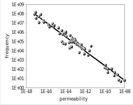
Figure 1: The transition frequency $f_{c}=\omega_{c}/2\pi$ (in $Hz$) predicted in the present study with $\omega_{c}$ from eq. 12 with $\eta=10^{-3}$ Pa.s and $\rho_{f}=10^{3}$ kg/m³ as a function of the permeability (in $m^{2}$). The transition frequency varies as $log_{10}(f_{c})=-0.78log_{10}(k)-5.5$. The parameters of the samples, $F$ and $k_{0}$ are measured from different authors on various samples cited in Tables 1, 2 and 3

We calculated the predicted transition frequency $f_{c}=\omega_{c}/2\pi$ with $\omega_{c}$ from eq. 12 with $\eta=10^{-3}$ Pa.s and $\rho_{f}=10^{3}$ kg/m³. The other parameters $F$ and $k_{0}$ are measured from different authors cited in Bernabé (1991) (see Table 2). We also calculated the parameters for four Fontainebleau sandstone samples. It has been shown for these samples that $F=\phi^{-2.01}$ (from Ruffet et al. (1991)) and that $k_{0}=a\phi^{n}$ with different values for $n$ according to the porosity. The following laws were chosen: $k_{0}=1.66$x$10^{-4}\phi^{8}$ for $\phi<6\%$ and $k_{0}=2.5$x$10^{-10}\phi^{3}$ for $\phi$ ranging between $8$ and $25\%$ (Bourbié et al., 1987). We can see that the transition frequencies are of the order of kHz and MHz and no more from 0.2 to 150 Hz as measured or calculated on glass beads, sand grains, crushed glass or capillaries. We plotted the results of the transition frequency as a function of the permeability on these various samples in Fig. 1. Although the formation factor is not constant with the permeability, it is clear that the transition frequency is inversely poportional to the permeability as:

$$log_{10}(f_{c})=-0.78log_{10}(k)-5.5$$ (19)

and varies from about $100$ MHz for $10^{-17}$ m² to about $10$ Hz for $10^{-8}$ m², so by seven orders of magnitude for nine orders of magnitude in permeability.

3 Experimental apparatus and procedure

Several experimental setups were proposed to provide the sinusoidal pressure variations.

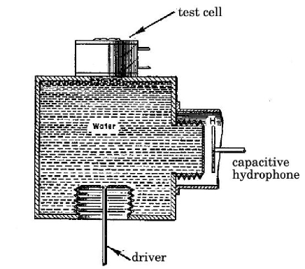
Figure 2: The sylphon bellows is driven by a geophone-type push-pull driver to apply a sinusoidal motion to the sample. (modified from Packard (1953))

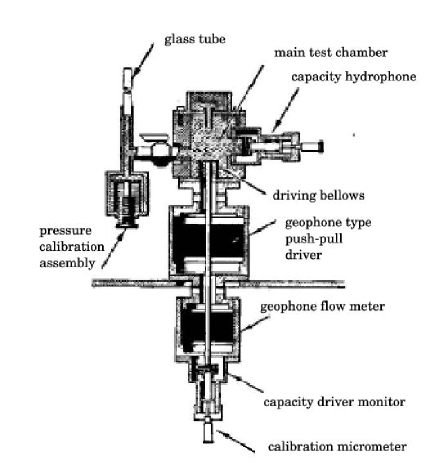
Figure 3: Experimental setup used by Thurston (1952a) (modified from Thurston (1952a)).

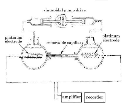
Figure 4: Experimental setup used by Groves & Sears (1975) (modified from Groves & Sears (1975)).

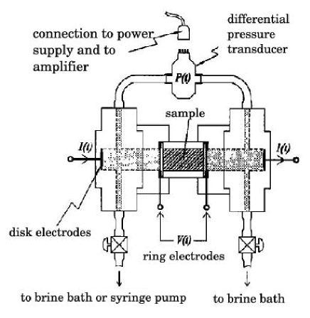
Figure 5: Experimental setup used by Pengra et al. (1999) for streaming potential and electro-osmosis measurements (modified from Pengra et al. (1999)).

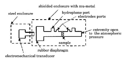
Figure 6: Experimental setup used by Reppert et al. (2001) (modified from Reppert et al. (2001)).

The first experimental apparatus proposed a sinusoidal motion delivered by a sylphon bellows which was driven by a geophone-type push-pull driver (Fig. 2 from Packard (1953)). The low frequency oscillator ($0.01$ Hz to $1$ kHz) was used for operation of the push-pull geophone driver. Similar setups were proposed by Thurston (1952b) (Fig. 3) and Cooke (1955), so that frequency of this kind of source was $1$-$400$ Hz (Cooke, 1955), $20$-$200$ Hz (Packard, 1953) and $10$-$700$Hz (Thurston, 1952b). The induced pressure was up to $2$ kPa. More recently Schoemaker et al. (2007) used a so-called Dynamic Darcy Cell (DCC) with a mechanical shaker connected to a rubber membrane leading to a frequency range for the oscillating pressure $5$ to $200$ Hz. The sinusoidal fluid flow was also applied by a displacement piston pump directly connected to the electrodes chambers (fig. 4 from Groves & Sears (1975); Sears & Groves (1978)). The piston was mounted on a Scotch Yoke drive attached to a controllable speed AC motor (Cerda & Non-Chhom, 1989). The frequency range of this source was then $0.4$Hz to $21$ Hz and the pressure up to $15$ kPa. Pengra et al. (1999) used a piston rod attached to a loudspeaker driven by an audio power amplifier (Fig. 5). They performed measurements up to $100$Hz, with an applied pressure of $5$ kPa RMS. More recently it was proposed by Reppert et al. (2001) to use an electromechanical transducer (fig. 6), and these authors covered a frequency range $1$-$500$ Hz. The vibrating exciter proposed by Schoemaker et al. (2008) was used from $5$Hz to $200$Hz. Recently Tardif et al. (2011) used an electromagnetic shaker operating in the range $1$Hz to $1$kHz and provided measurements up to $200$Hz. Higher frequencies have been investigated (Zhu et al., 1999, 2000; Chen & Mu, 2005; Block & Harris, 2006; Zhu et al., 2008) for the detection of the interfacial conversions.

The electromagnetic noise radiating from such equipment must be suppressed by shielding the set-up and wires (shielded twisted cable pairs) (Tardif et al., 2011; Schoemaker et al., 2008). Moreover it is essential to have a rigid framework. A mechanical resonance can occur in the cell/transducer system (at $70$Hz in Pengra et al. (1999)), and the noise associated with mechanical vibration can be suppressed puting an additional mass to the frame (Tardif et al., 2011).

Once the oscillatory pressure is applied, the pressure must be measured. Most of the setups include piezoelectric transducers to measure the pressure difference over the capillary or the porous sample. Reppert et al. (2001) proposed to use hydrophones that have a flat response from $1$ to $20$ kHz. Tardif et al. (2011) proposed to use dynamic transducers with a low-frequency limit $0.08$ Hz and a maximum frequency of $170$ kHz.

The electrodes are usually Ag/AgCl or platinium electrodes. The electrodes used by Schoemaker et al. (2008) were sintered plates of Monel (composed of nickel and copper). The electrical signal must be measured using pre-amplifiers or a high-input impedance acquisition system. Since the impedance of the sample depends on the frequency, one must correct the measurements from this varying-impedance to be able to have a correct streaming potential coefficient (Reppert et al., 2001). Moreover the electrodes at top and bottom of the sample can behave as a capacitor, requiring a correction using impedance measurements too (Schoemaker et al., 2008).

The sample is usually saturated and it is emphasized that the sample should be left until equilibrium with water. This equilibrium can be obtained by leaving the sample in contact with water for some time, and by flowing the water within the sample several times by checking the $pH$ and the water conductivity until an equilibrium is reached (Guichet et al., 2003). The procedure including water flow is better because the properties of the water can be measured. When the properties of the water are measured only before saturating the sample, the resulting water once in contact with the sample is not known. Usually the water is more conductive when in contact with the sample, and the $pH$ can change. Recalling that the streaming potential is proportional to the zeta potential (which depends on $pH$) and inversely proportional to the water conductivity (eq.1), it is essential to know properly the $pH$ and the water conductivity.

4 Measurements and calculations of the dynamic electrokinetic coefficient

The absolute magnitude of the streaming potential coefficient normalized by the steady-state value was calculated by Packard (1953) as:

$$f(Y_{a})=\left(\frac{-2}{Y_{a}}\frac{i\sqrt{i}J_{1}(\sqrt{i}Y_{a})}{J_{0}(\sqrt{i}Y_{a})}e^{-i\omega t}\right)$$ (20)

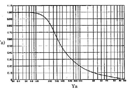
Figure 7: The absolute magnitude of the normalized streaming potential coefficient calculated by Packard (1953) using eq. 20 where $Y_{a}=a\sqrt{\frac{\omega\rho_{f}}{\eta}}$, equivalent to eq. 2 (modified from Packard (1953))

which is equal to eq. 2, but expressed as a function of the parameter $Y_{a}=a\sqrt{\frac{\omega\rho_{f}}{\eta}}$, the transition frequency being obtained for $Y_{a}=1$ (Fig. 7). The streaming potential coefficient is constant up to the transition angular frequency, and then decreases with increasing frequency.

Sears & Groves (1978) measured the streaming potential coefficient on a capillary of radius $508$ $\micron$ which was coated with clay-Adams Siliclad and then incubated with 1% bovine serum albumin, and filled with 0.02 $M$ Tris-HCl at $pH$ $7.32$. They reported the streaming potential and the pressure difference as a function of frequency in the range $0-20$ Hz. We calculated the resulting streaming potential coefficient (see Fig. 8) which decreases from about $1.3$x $10^{-7}$ to $4$x $10^{-8}$ V/Pa. These authors computed the zeta potential and concluded that the zeta potential is independent of the frequency with an average value of $28.8$ mV. Moreover they concluded that the zeta potential is also independent of the capillary radius and capillary length.

The value of the streaming potential coefficient on Ottawa sand measured at 5 Hz by Tardif et al. (2011) was $-5.2$x $10^{-7}$ V/Pa using a 0.001 mol/L NaCl solution to saturate the sample. Values between $1$ and $2$x$10^{-8}$ V/Pa were measured on samples saturated by $0.1$ M/L NaCl brine (Pengra et al., 1999). A compilation of numerous streaming potential coefficients measured on sands and sandstones at various salinities in DC domain (Allègre et al., 2010) showed that $C_{s0}=-1.2$ x $10^{-8}\sigma_{f}^{-1}$, where $C_{s0}$ is in V/Pa and $\sigma_{f}$ in S/m. A zeta potential of $-17$mV can be inferred from these collected data, assuming the other parameters (see eq. 1) independent of water conductivity. These assumptions are not exact, but the value of zeta is needed for numerous modellings which usually assume the other parameters independent of the fluid conductivity. Therefore an average value of $-17$ mV for such modellings can be rather exact, at least for medium with no clay nor calcite.

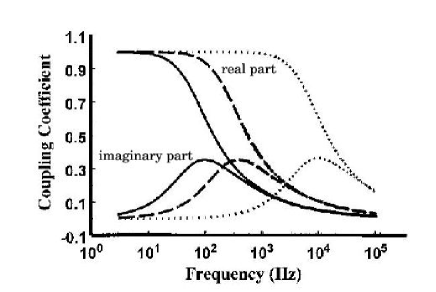
Figure 9: The real and imaginary part of the Packard’s model (eq.2) calculated by Reppert et al. (2001) for three capillary radii: 100(continuous line), 50(dashed line), 10(point line) (modified from Reppert et al. (2001)).

Reppert et al. (2001) calculated the real part and the imaginary part of the theoretical Packard’s streaming potential coefficient (eq. 2) for different capillary radii. (see Fig. 9). It can be seen that the larger the radius is, the lower the transition frequency is, as shown above by the different theories. Recent developments by the group of Glover have been performed to build a new setup and to make further measurements on porous samples: two papers detail these studies in this special issue on Electrokinetics in Earth Sciences.

5 Conclusion

Since the theory of Pride in 1994, the dynamic behavior of the streaming potential is known for porous media. However few experimental results are avalaible, because of the difficulty to perform correct measurements at high frequency. Up to now, measurements of the frequency-dependence of the streaming potential have been performed up to $200$ Hz on high-permeable samples. The main difficulty arises from electrical noise induced by mechanical vibration. Moreover it has been emphasized that the measurements must be corrected by impedance measurements as a function of frequency too because the impedance of the sample depends on frequency. Further theoretical developments performed by Garambois & Dietrich (2001) studied the low frequency assumption valid at frequencies lower than the transition frequency. We show that this transition frequency, on a various collection of samples for which both formation factor and permeability are measured, is predicted to depend on the permeability as inversely proportional to the permeability.

6 Acknowledgements

This work was supported by the French National Scientific Center (CNRS), by the National Agency for Research (ANR) through TRANSEK, and by REALISE the “Alsace Region Research Network in Environmental Sciences in Engineering” and the Alsace Region. We thank two anonymous reviewers and the associate editor T. Ishido for very constructive remarks that improved this paper.

7 References

Table 1: Measured or predicted transition frequency for dynamic streaming potential and permeability, for samples of porosity $\phi$, formation factor $F$, permeability $k_{0}$, and half of the mean particle size r, from (SED) Smeulders et al. (1992), (CKS) Charlaix et al. (1988), (SG) Sears & Groves (1978), (P)Packard (1953), (TGR) Tardif et al. (2011), (RMLJ) Reppert et al. (2001). ^∗ indicates predicted transition frequency from eq. 3 and ^∗∗ indicates the transition frequency computed by the authors.

Sample	particle size $\mu m$	$\phi$ [%]	$F$	$k_{0}$ [m2]	$f_{c}$ [Hz]	source
capillary	254(radius)			10-8	10-2.5∗ Hz	CKS
capillary	508(radius)				1.3-0.62∗ Hz	SG
capillary G4	720(radius)				0.31∗-0.28 ∗∗ Hz	P
capillary G2	826(radius)				0.23∗-0.21 ∗∗ Hz	P
capillary 1	800-1100(radius)				7.1 Hz	RMLJ
glass beads	1.25-1.75	32	7.8	4.2x10-9	4.8 Hz	SED
glass beads	850 (r)	50	2.8	10-8	6.2 Hz	CKS
glass beads	580-700	31	8.7	9x10-10	20 Hz	SED
glass beads	450 (r)	50	3.2	2x10-9	25 Hz	CKS
glass beads	250 (r)	50	3	5x10-10	108 Hz	CKS
glass beads	200-270	31	9	1.4x10-10	126 Hz	SED
crushed glass	440 (r)	50	3	10-9	44 Hz	CKS
crushed glass	265 (r)	50	3.2	2x10-10	45-103 Hz	CKS
porous fliter A	72.5-87				269 Hz	RMLJ
porous fliter B	35-50				710 Hz	RMLJ
sand grains	1000-2000	31	9	26x10-10	6.7 Hz	SED
sand grains	150-300	29	10.7	10-10	149 Hz	SED
Ottawa sand	200-250 (r)	31	4.7	1.2x10-10	230-273 Hz	TGR

Table 2: Predicted transition frequency (from eq. 12) for dynamic streaming potential, for samples of porosity $\phi$, formation factor $F$ and permeability $k_{0}$, from (1) calculated in the present study, and measured by (2) Taherian et al. (1990), (3) Morgan et al. (1990), (4)Fatt (1957), (5)Wyble (1958), (6)Dobrynin (1962), (7)Chierici et al. (1967), (8)Yale (1984).

Sample	$\phi$ [%]	$F$	$k_{0}$ [m2]	$f_{c}$ [Hz]
Fontainebleau sandstone1	20	25	2x10-12	3.2 kHz
Fontainebleau sandstone1	15	45	8x10-13	4.4 kHz
Fontainebleau sandstone1	10	102	2.5x10-13	6.2 kHz
sandstone-S222	31.2	6	2.7x10-12	9.7 kHz
sandstone-S472	20	14.4	8.5x10-13	13 kHz
Boise8	26	12	9x10-13	14.7 kHz
Berea sandstone5008	20	20	4.9x10-13	16.2 kHz
sandstone-S422	19.7	14.7	6.7x10-13	16.2 kHz
sandstone-S452	21	11.7	7.2x10-13	18.8 kHz
Fahler 1628	3	294	2.7x10-14	20 kHz
sandstone-S432	21.2	13	5.1x10-13	23.5 kHz
Pliocene 417	21	144.9	4.2x10-14	26.1 kHz
Pliocene 357	20	156.2	3.7x10-14	27.5 kHz
Berea sandstoneC2H3	19.8	15.1	3.8x10-13	27.7 kHz
sandstone-S502	18.3	17.2	3.1x10-13	30 kHz
Triassic387	21	12.6	4x10-12	31.4 kHz
Triassic347	20	13.9	3.5x10-13	32.7 kHz
Berea sandstoneB23	20.3	15.2	2.64x10-13	39.7 kHz
sandstone-S52	26.4	8.7	4.1x10-13	45 kHz
sandstone-S352	18.75	17.4	2x10-13	46.5 kHz
Massillon DH8	16	23.8	1.3x10-13	51.4 kHz
Cambrian 167	14	312.5	9.5x10-15	53.6 kHz
Fontainebleau sandstone1	5	412	6.5x10-15	59.4 kHz
Berea sandstoneD13	18.5	18.4	1.3x10-13	66.5 kHz
Tensleep14	15	18.9	1.2x10-13	70.3 kHz
Tertiary 8078	22	14.9	1.5x10-13	71.1 kHz
Cambrian 67	8.1	90.9	2.3x10-14	76.1 kHz

Table 3: continued

Sample	$\phi$ [%]	$F$	$k_{0}$ [m2]	$f_{c}$ [Hz]
Torpedo6	20	41.7	4.5x10-14	84.9 kHz
Miocene 77	8.3	384.6	4.4x10-15	94 kHz
Cambrian 147	11	52.6	3.2x10-14	94.5 kHz
sandstone Triassic277	18	20	7.2x10-14	110.5 kHz
sandstone-S92	20.9	12	1x10-13	126.2 kHz
Triassic267	18	17.2	6.8x10-14	135.7 kHz
sandstone-S62	22.8	10.6	8.3x10-14	180.7 kHz
Berea 100H8	17	17.2	4.9x10-14	188.4 kHz
sandstone S152	21.8	13.9	4.5x10-14	256.7 kHz
Kirkwood5	15	40	1.2x10-14	331.6 kHz
Indiana DV8	27	12	3x10-14	440.3 kHz
Island Rust A13	14.6	52.5	5.2x10-15	579 kHz
Bradford5	11	90	2.5x10-15	700.3 kHz
Austin chalk3	23.6	22.7	9.7x10-15	763 kHz
Massillon DV8	19	27.8	6.9x10-15	830.4 kHz
sandstone-S342	21.35	13.7	1.1x10-14	1.06 MHz
sandstone S442	15.7	24.5	4.2x10-15	1.5 MHz
Indiana L. SA13	18	29.2	1.9x10-15	2.9 MHz
Tennessee A13	5.5	180.3	2.3x10-16	3.8 MHz
AZPink (Coconino)3	10.3	62.4	6.3x10-16	4.04 MHz
Leuders L.SA13	15.2	41.5	7.1x10-16	5.3 MHz
sandstone-S402	10.9	130	1.9x10-16	6.4 MHz
sandstone-S232	18.8	40.7	4.8x10-16	8.1 MHz
Fahler 1898	1.9	714.3	2x10-17	11.1 MHz
Penn blue A13	3.9	219	6.2x10-17	11.7 MHz
AZChoclate23	9.5	159.3	5.8x10-17	17.2 MHz
Fahler 1618	2.3	416.7	1x10-17	38.2 MHz
Fahler 1428	7.6	164	2x10-17	48.5 MHz
sandstone S212	12.1	65	3x10-17	81.7 MHz
Fahler 1548	4.6	263.1	7x10-18	86.4 MHz
Fahler 1928	4.4	128.2	9x10-18	137.9 MHz

Figure 8: The streaming potential coefficient measured as a function of frequency by Sears & Groves (1978) on a capillary coated with clay, incubated with BSA in 0.02 M Tris-HCl.

References

- Allègre et al. (2010) Allègre, V., Jouniaux, L., Lehmann, F., & Sailhac, P., 2010. Streaming Potential dependence on water-content in fontainebleau sand, Geophys. J. Int., 182, 1248–1266.
- Allègre et al. (2011) Allègre, V., Jouniaux, L., Lehmann, F., & Sailhac, P., 2011. Reply to the comment by A. Revil and N. Linde on: ”Streaming potential dependence on water-content in fontainebleau sand” by Allègre et al., Geophys. J. Int., 186, 115–117.
- Auriault et al. (1985) Auriault, J., Borne, L., & Chambon, R., 1985. Dynamics of porous saturated media, checking of the generalized law of darcy, J. Acoust. Soc. Am., 77, 1641–1650.
- Bernabé (1991) Bernabé, Y., 1991. Pore geometry and pressure dependence of the transport properties in sandstones, Geophysics, 56, 436–446.
- Biot (1956) Biot, M. A., 1956. Theory of propagation of elastic waves in a fluid-saturated porous solid: I. low frequency range, J. Acoust. Soc. Am., 28(2), 168–178.
- Block & Harris (2006) Block, G. I. & Harris, J. G., 2006. Conductivity dependence of seismoelectric wave phenomena in fluid-saturated sediments, J. Geophys. Res., 111, B01304.
- Bordes et al. (2006) Bordes, C., Jouniaux, L., Dietrich, M., Pozzi, J.-P., & Garambois, S., 2006. First laboratory measurements of seismo-magnetic conversions in fluid-filled Fontainebleau sand, Geophys. Res. Lett., 33, L01302.
- Bordes et al. (2008) Bordes, C., Jouniaux, L., Garambois, S., Dietrich, M., Pozzi, J.-P., & Gaffet, S., 2008. Evidence of the theoretically predicted seismo-magnetic conversion, Geophys. J. Int., 174, 489–504.
- Bourbié et al. (1987) Bourbié, T., Coussy, O., & Zinszner, B., 1987. Acoustic of porous media, Institut Francais du pétrole publications, Ed. Technip.
- Cerda & Non-Chhom (1989) Cerda, C. & Non-Chhom, K., 1989. The use of sinusoidal streaming flow measurements to determine the electrokinetic properties of porous media, Colloids and Surfaces, 35, 7–15.
- Chandler (1981) Chandler, R., 1981. Transient streaming potential measurements on fluid-saturated porous structures: An experimental verification of Biot’s slow wave in the quasi-static limit, J. Acoust. Soc. Am., 70, 116–121.
- Charlaix et al. (1988) Charlaix, E., Kushnick, A. P., & Stokes, J., 1988. Experimental study of dynamic permeability in porous media, Phys. Rev. Lett., 61(14), 1595–1598.
- Chen & Mu (2005) Chen, B. & Mu, Y., 2005. Experimental studies of seismoelectric effects in fluid-saturated porous media, J. Geophys. Eng., 2, 222–230.
- Chierici et al. (1967) Chierici, G., Ciucci, G., Eva, F., & Long, G., 1967. Effect of the overburden pressure on some petrophysical parameters of reservoir rocks, Proc. 7th World Petroleum Cong., 2, 309–338.
- Cooke (1955) Cooke, C. E., 1955. Study of electrokinetic effects using sinusoidal pressure and voltage, J. Chem. Phys., (23), 2299–2303.
- Davis et al. (1978) Davis, J. A., James, R. O., & Leckie, J., 1978. Surface ionization and complexation at the oxide/water interface, J. Colloid Interface Sci., 63, 480–499.
- Dobrynin (1962) Dobrynin, V., 1962. Effect of overburden pressure on some properties of sandstones, Soc. Petr. Engrs. J., (2), 360–366.
- Dupuis & Butler (2006) Dupuis, J. C. & Butler, K. E., 2006. Vertical seismoelectric profiling in a borehole penetrating glaciofluvial sediments, Geophys. Res. Lett., 33.
- Dupuis et al. (2007) Dupuis, J. C., Butler, K. E., & Kepic, A. W., 2007. Seismoelectric imaging of the vadose zone of a sand aquifer, Geophysics, 72, A81–A85.
- Dupuis et al. (2009) Dupuis, J. C., Butler, K. E., Kepic, A. W., & Harris, B. D., 2009. Anatomy of a seismoelectric conversion: Measurements and conceptual modeling in boreholes penetrating a sandy aquifer, J. Geophys. Res. Solid Earth, 114(B13), B10306.
- Fatt (1957) Fatt, I., 1957. Effect of overburden and reservoir pressure on electric logging formation factor, Bull. Am. Ass. Pet. Geol., 41, 2456–2466.
- Fenoglio et al. (1995) Fenoglio, M., Johnston, M., & Byerlee, J., 1995. Magnetic and electric fields associated with changes in high pore pressure in fault zones; application to the loma prieta ulf emissions, J. Geophys. Res., 100, 12951–12958.
- Gao & Hu (2010) Gao, Y. & Hu, H., 2010. Seismoelectromagnetic waves radiated by a double couple source in a saturated porous medium, Geophys. J. Int., 181, 873–896.