The quantum $J_{1}-J_{1}^{\prime}-J_{2}$ spin-$1/2$ Heisenberg antiferromagnet: A variational method  study

Abstract

The phase transition of the quantum spin-$1/2$ frustrated Heisenberg antiferroferromagnet on an anisotropic square lattice is studied by using a variational treatment. The model is described by the Heisenberg Hamiltonian with two antiferromagnetic interactions: nearest-neighbor (NN) with different coupling strengths $J_{1}$ and $J_{1}^{\prime}$ along x and y directions competing with a next-nearest-neighbor coupling $J_{2}$ (NNN). The ground state phase diagram in the ($\lambda,\alpha$) space, where $\lambda=J_{1}^{\prime}/J_{1}$ and $\alpha=J_{2}/J_{1}$, is obtained. Depending on the values of $\lambda$ and $\alpha$, we obtain three different states: antiferromagnetic (AF), collinear antiferromagnetic (CAF) and quantum paramagnetic (QP). For an intermediate region $\lambda_{1}<\lambda<1$ we observe a QP state between the ordered AF and CAF phases, which disappears for $\lambda$ above some critical value $\lambda_{1}$. The boundaries between these ordered phases merge at the quantum critical endpoint (QCE). Below this QCE there is again a direct first-order transition between the AF and CAF phases, with a behavior approximately described by the classical line $\alpha_{c}\simeq\lambda/2$.

PACS numbers: 75.10.Jm, 05.30.-d, 75.40.-s, 75.40.Cx

I Introduction

The study of the phase transition of frustrated spin systems on two-dimensional (2d) lattices is a central problem in modern condensed mater physics. A competition of exchange interaction can lead to frustration, where spatial arrangement of magnetic ions in a crystal for which a simultaneous antiparallel ordering of all interacting spin is impossible. In particular, one of the frustrated 2d models most discussed is the quantum spin-$1/2$ Heisenberg antiferromagnet on a square lattice with competing nearest-neighbor (NN) and next-nearest-neighbor (NNN) antiferromagnetic exchange interactions (known as $J_{1}-J_{2}$ model) 1 ; 3 ; 4 ; 5 ; 6 ; 7 ; 8 ; 9 ; 10 ; 11 ; 12 ; bishop1 ; darradi ; isaev ; viana ; oliveira .

The criticality of this $J_{1}-J_{2}$ Heisenberg model on a square lattice are relatively well known at $T=0$.  There are two magnetically long-range ordered phases at small and at large values of $\alpha=J_{2}/J_{1}$ separated by an intermediate quantum paramagnetic phase without magnetic long-range order in the region between $\alpha_{1c}\simeq 0.4$ and $\alpha_{2c}\simeq 0.6$, where the properties of these disordered phase are still under intensive debate. For $\alpha<$ $\alpha_{1c}$, the system possesses antiferromagnetic (AF) long-range order with wave vector $\mathbf{Q}=(\pi,\pi)$, with a staggered magnetization smaller than the saturated value (quantum fluctuations), which vanished continuously when $\alpha\rightarrow\alpha_{1c}$. For $\alpha>\alpha_{2c}$ we have two degenerate collinear states which are the helical states with pitch vectors $\mathbf{Q}=(\pi,0)$ and $(0,\pi)$. These two collinear states are characterized by a parallel spin orientation of nearest neighbors in vertical (or horizontal) direction and an antiparallel spin orientation of nearest neighbors in horizontal (or vertical) direction, and therefore exhibit Néel order within the initial sublattice A and B. At $\alpha=\alpha_{2c}$, the magnetization jumps from a nonzero to a zero value. The phase transition from Néel to the quantum paramagnetic state is second order, whereas the transition from the collinear to the quantum paramagnetic state is first orderviana ; oliveira . Isaev, et al.isaev have shown that the intermediate quantum paramagnetic is a (singlet) plaquette crystal, and the ground and first excited states are separated by a finite gap.

The interest to study the two-dimensional $J_{1}-J_{2}$ Heisenberg antiferromagnet have been greatly stimulated by its experimental realization in vanadium phosphates compoundsmelzi ; carretta ; rosner ; bombardi , such as Li₂VOSiO₄, Li₂VOGeO₄, and  VOMoO₄, which might be described by this frustrated model in the case of $J_{2}\simeq J_{1}$ ($\alpha=J_{2}/J_{1}\simeq 1$). These isostructural compounds are characterized by a layered structure containing V⁴⁺ ($S=1/2$) ions. The structure of V⁴⁺ layer suggest that the superexchange is similar. In these compounds a second order phase transition to a long-range ordered magnetic phase has been observed. NMR spin-lattice relaxation measurementsmelzi below $T_{c}$ shows that the order is collinear. Due to the two-fold degeneracy of the ground-state for $\alpha>0.7$ it is not possible to say a priori which will be the magnetic wave vector (i.e., $\mathbf{Q}=(\pi,0)$ and $(0,\pi)$) below $T_{c}$. On the other hand, such a scenario can change by considering spin-lattice coupling which will lift the degeneracy of the ground-state and will lower its energybecca . Then, any structural distortion should inevitably reduce this competing interactions and thus reduces the frustration. In the case of  this frustrated magnetic materials, the competing interactions are inequivalent but their topology and magnitudes can be tuned so that the strong quantum fluctuations destroy the long-range ordering. Experimentally the ground state phase diagram of frustrated compounds, described by the $J_{1}-J_{2}$ model, can be explored continuously from high to the low $\alpha=J_{2}/J_{1}$ regime by applying high pressures (P), which modify the bonding lengths and angles. Recent results from x-ray diffraction measurementspavarini on the Li₂VOSiO₄ compound has shown that the ratio $\alpha$ decreases by about $40\%$ when the pressure increases from $0$ to $7.6$GPa.

A generalization of the $J_{1}-J_{2}$ Heisenberg antiferromagnetic model on a square lattice was introduced by Nersesyan and Tsveliknerseyan and studied by other groupsequivalence1 ; equivalence2 ; equivalence3 ; equivalence4 ; equivalence5 ; equivalence6 ; equivalence7 ; equivalence8 , the so-called $J_{1}-J_{1}^{\prime}-J_{2}$ model. In the $J_{1}-J_{1}^{\prime}-J_{2}$ model is considered inequivalence nn couplings $J_{1}$ and $J_{1}^{\prime}=\lambda J_{1}$ in the two orthogonal spatial lattice dimensions with all the NNN bonds across the diagonals to have the same strength $J_{2}$. Study of extensive band structure calculationsequivalence6 for the vanadium phosphates ABVO(PO₄)₂ (AB=Pb₂, SrZn, BaZn, and BaCd) have indicated four inequivalent exchange couplings: $J_{1}$ and $J_{1}^{\prime}$ between NN and $J_{2}$ and $J_{2}^{\prime}$ between NNN. For example, in SrZnVO(PO₄)₂ was estimated $J_{1}^{\prime}/J_{1}\simeq 0.7$ and $J_{2}^{\prime}/J_{2}\simeq 0.4$ causing a distortion of the spin lattice. This spatial anisotropy tends to narrow the critical region and destroys it completely at a certain value of the interchain parameter $\lambda$.

On the other hand, by using the continuum limit of the $J_{1}-J_{1}^{\prime}-J_{2}$ spin-$1/2$ model Starykh and Balentsequivalence1 have shown that this transition splits into two, with the presence of an intermediate quantum paramagnetic (columnar dimer) phase for $\lambda\leq 1$. Bishop, et alequivalence4 , by using coupled cluster treatment found the surprising and novel result that there exists a quantum triple point (QTP) with coordinates at ($\alpha_{t}=0.33\pm 0.02,\lambda_{t}=0.60\pm 0.03$), below which there is a second-order phase transition between the AF and CAF phases while above this QTP are these two ordered phases separated by the intermediate magnetically disordered phase (VBS or RVB). The order parameters of both the AF and CAF phases vanish continuously both below and above the QTP, which is typical of second-order phase transition. There is some evidence that the transition between the CAF and intermediate phases is of first-order. Using exact diagonalizationequivalence2 with small lattice of $N\leq 36$ ($6\times 6$) size, the intermediate QP phase for all interval of $\lambda\in[0,1]$ has been obtained for the pure spin-$1/2$ $J_{1}-J_{2}$ model on a square lattice. These results are in accordance with results obtained by Starykh and Balentesequivalence1 , that predicted not the QTP in the ground-state phase diagram recently observed by Bishop, et al.equivalence4 .

The ground state (GS) properties of the two-dimensional frustrated Heisenberg antiferromagnet have been investigated by various methods. The exact diagonalization starts from singlet states on pairs of sites, which cover the whole 2d lattice. However, the manifold of these states which can be constructed is nonorthogonal and overcomplete. This numerical methods are limited to small clusters $N\leq 6\times 6=36$ due to storage problems. The computation on the largest cluster $6\times 6$ has been performed by Schulz and co-workes3 $20$ years ago. In spite of the great improvements achieved during this time, it is not possible so far to repeat this calculation for the next interesting cluster $8\times 8$. This is only possible with other technique, as the quantum Monte Carlo simulation. Due to the progress in computer hardware and the increased efficiency in programing, very recentlyexact the GS of the quantum spin-1/2 $J_{1}-J_{2}$ model have been calculated by the Lanczos algoritm for a square lattice with $N=40$  sites.

The theoretical treatment of the frustrated quantum models is far from being trivial. Many of the standard many-body methods, such as quantum Monte Carlo techniques, may fail or become computationally infeasible to implement if frustration is present due to the minus-sign problem. Hence, there is considerable interest in any method that can deal with frustrated spin systems. This considerable qualitative difference in the ground state phase diagram in the $\alpha-\lambda$ plane of the quantum spin-$1/2$ $J_{1}-J_{1}^{\prime}-J_{2}$ model further motivates us to study this issue by alternative methods.

Using a variational approximation, in which plaquettes of four spins are treated exactly, Oliveiraoliveira has studied the ground state phase diagram of the pure $J_{1}-J_{2}$ Heisenberg antiferromagnet on a square lattice, where the quantitative results are in good accordance with a more sophisticated method (exact diagonalization). In this work, we generalize this variational method to treat the anisotropic square lattice ( $J_{1}-J_{1}^{\prime}-J_{2}$ model). The rest of this paper is organized as follows: In Sec. II, the model is presented and a brief discussion of results. In Sec. III, the method is applied for the case of one plaquette with four spins interacting with other plaquette type mean field approximation. Main results will be presented in Sec. IV, as well as some discussions. Finally, in Sec. V we will give a brief summary.

II Model

The critical behavior of the quantum spin-$1/2$ $J_{1}-J_{2}$ Heisenberg model has been studied for many years, but very little has been done in the anisotropic square lattice case, which is described by following Hamiltonian:

$$\mathcal{H}={\textstyle\sum\limits_{\left\langle i,j\right\rangle}}\left(J_{1}\mathbf{\sigma}_{i,j}\cdot\mathbf{\sigma}_{i+1,j}+J_{1}^{\prime}\mathbf{\sigma}_{i,j}\cdot\mathbf{\sigma}_{i,j+1}\right)+J_{2}{\textstyle\sum\limits_{\left\langle\left\langle i,j\right\rangle\right\rangle}}\left(\mathbf{\sigma}_{i,j}\cdot\mathbf{\sigma}_{i+1,j+1}+\mathbf{\sigma}_{i+1,j}\cdot\mathbf{\sigma}_{i,j+1}\right),$$ (1)

where $\mathbf{\sigma}_{i,j}\mathbf{=}(\sigma_{i,j}^{x},\sigma_{i,j}^{y},\sigma_{i,j}^{z})$ is the spin-$1/2$ Pauli spin operators, the index $(i,j)$ labels the $x$ (row) and $y$ (column) components of the lattice sites. The first sum runs over all NN and the second sum runs over all NNN pairs. We denote the Hamiltonian (1)  by $J_{1}-J_{1}^{\prime}-J_{2}$ model, with strength $J_{1}$ along the row direction, $J_{1}^{\prime}=\lambda J_{1}$ along the column direction, $J_{2}=\alpha J_{1}$ along the diagonals, and we assume all couplings to be positive with $J_{1}^{\prime}<J_{1}$.

The classical ($S=\infty$) model (1) has only two ordered ground-states: AF (or Néel) for $\alpha>\lambda/2$ and columnar stripe (CAF) for $\alpha<\lambda/2$ separated by a first-order line at $\alpha_{c}=\lambda/2$. Quantum fluctuations play a significant role in the magnetic phase diagram of the system at zero temperature. We will investigate the role of quantum fluctuations on the stability of the Néel and collinear phases. In the $S=1/2$ case (quantum limit), the line splits into two phase transitions, where the ordered states (AF and CAF) are separated by an intermediate quantum paramagnetic (QP) phase, both on a square lattice. Exact diagonalization12 has estimated a critical line at $\alpha_{CAF}=\alpha_{c}+\frac{5\lambda^{2}}{8\pi^{2}}$, for the transition between the CAF and QP states, and at $\alpha_{AF}=\alpha_{c}-\frac{\lambda^{2}}{8\pi^{2}}$ between the AF and QP states. The phase diagram in the $\alpha-\lambda$ plane obtained is in accordance with Starykh and Balentsequivalence1 . However, the existence of QTP (quantum triple point) that was predicted by Bishop, et al.equivalence4 , is not present in their obtained phase diagram. Moreover, they found only presence of second-order phase transitions in the phase diagram. This contradictory qualitative results (existence or not of QTP) is the primary motivation behind this present work.

On the other hand, a critical endpoint (CE) is a point in the phase diagram where a critical line meets and is truncated by a first-order line. This CE appear in the phase diagram of many physical systems such as binary fluid mixtures, superfluids, binary alloys, liquid crystals, certain ferromagnets, etc, and have been known for over a centuryce1 . Despite the CE long history, new singularities at the CE were predicted. Fisher and Uptonce2 argued that a new singularity in the curvature of the first-order phase transition line should arise at a CE. This prediction was confirmed by Fisher and Barbosa’sce3 phenomenological studies for an exactly solvable spherical model. In conclusion of the analysis of the multicritical behavior observed in the ground-state phase diagram in the $\lambda-\alpha$ plane for the $J_{1}-J_{1}^{\prime}-J_{2}$ model, we have the presence of a quantum critical endpoint (QCE) and not QTP as mentioned other worksequivalence4 ; equivalence8 Therefore, the objective of this work is to obtain the QCE using the variational method, that was developed previously by Oliveiraoliveira in the pure limit ($\lambda=1$) case.

III Method

We first express the fluctuations around the classical ground state (AF and CAF phases), where consider a trial vector state $\left|\Psi_{0}\right\rangle=\prod\limits_{l=1}^{N/4}\left|\phi_{0l}\right\rangle$ for the ground state as a product of plaquette state $\left|\phi_{0l}\right\rangle$ . We denote the plaquettes by $l$ label, that is composed of four spins, where it do not overlap (mean field) on the square lattice as illustrated in figure 1. Each plaquette state is given by

Figure 1: Two-dimensional square lattice with a plaquette structure to be considered in this paper. The negrit plaquette is composed with the four $\mathbf{\sigma}_{1},\mathbf{\sigma}_{2},\mathbf{\sigma}_{3},$ and $\mathbf{\sigma}_{4\text{ }}$ spin operators that are considered in Eq. (2).

$$\left|\phi_{0l}\right\rangle=\sum_{n=1}^{6}a_{n}\left|n\right\rangle_{l},$$ (2)

where {$\left|1\right\rangle=\left|+-+-\right\rangle$, $\left|2\right\rangle=\left|-+-+\right\rangle,\left|3\right\rangle=\left|++--\right\rangle,\left|4\right\rangle=\left|-++-\right\rangle,\left|5\right\rangle=\left|--++\right\rangle,\left|6\right\rangle=\left|+--+\right\rangle$} is the vector basis with $\sigma^{z}=\sum\limits_{i=1}^{4}\sigma_{i}^{z}=0$, {$a_{i}$} are real variational parameters obeying the normalization condition $\sum\limits_{n=1}^{6}a_{n}^{2}=1$. With this choice of vector states, the mean value of the spin operator in each site of the plaquette is given by $\left\langle\mathbf{\sigma}_{i}\right\rangle=m_{i}\widehat{z},$ $m_{i}=\left\langle\sigma_{i}^{z}\right\rangle=\left\langle\phi_{0l}\left|\sigma_{i}^{z}\right|\phi_{0l}\right\rangle$, where the components in the $x$ and $y$ directions are null.

Using the trial vector state defined in the Eq. (2), we obtain the magnetizations at each site that are given by

$$m_{1}=2\left(xu+yv-zw\right),$$ (3)

$$m_{2}=2\left(-xu+yv+zw\right),$$ (4)

$$m_{3}=2\left(xu-yv+zw\right),$$ (5)

and

$$m_{4}=2\left(-xu-yv+zw\right),$$ (6)

where we have used the same set of parameters (canonical transformation) of Ref.oliveira , i.e., $x=\left(a_{1}+a_{2}\right)/\sqrt{2},y=\left(a_{3}+a_{5}\right)/\sqrt{2},z=\left(a_{4}+a_{6}\right)/\sqrt{2},u=\left(a_{1}-a_{2}\right)/\sqrt{2},v=\left(a_{3}-a_{5}\right)/\sqrt{2}$, and $w=\left(a_{4}-a_{6}\right)/\sqrt{2}$, which obeys the normalization condition $x^{2}+y^{2}+z^{2}+u^{2}+v^{2}+w^{2}=1$.

The ground state energy per spin and unit of $J_{1}$, $E_{0}=\left\langle\Psi_{0}\left|\mathcal{H}\right|\Psi_{0}\right\rangle/NJ_{1}$, is given by

$$E_{0}=E_{01}+E_{02},$$ (7)

with

$$E_{01} =\left\langle\overrightarrow{\sigma}_{1}.\overrightarrow{\sigma}_{2}\right\rangle_{A}+\lambda\left\langle\overrightarrow{\sigma}_{2}.\overrightarrow{\sigma}_{3}\right\rangle_{A}+\left\langle\overrightarrow{\sigma}_{3}.\overrightarrow{\sigma}_{4}\right\rangle_{A}+\lambda\left\langle\overrightarrow{\sigma}_{4}.\overrightarrow{\sigma}_{1}\right\rangle_{A}+$$

$$\lambda\left\langle\overrightarrow{\sigma}_{1}\right\rangle_{A}.\left\langle\overrightarrow{\sigma}_{5}\right\rangle_{B}+\lambda\left\langle\overrightarrow{\sigma}_{2}\right\rangle_{A}.\left\langle\overrightarrow{\sigma}_{6}\right\rangle_{B}+\left\langle\overrightarrow{\sigma}_{2}\right\rangle_{A}.\left\langle\overrightarrow{\sigma}_{8}\right\rangle_{D}+\left\langle\overrightarrow{\sigma}_{3}\right\rangle_{A}.\left\langle\overrightarrow{\sigma}_{9}\right\rangle_{D},$$ (8)

and

$$E_{02} =\alpha\left[\left\langle\overrightarrow{\sigma}_{1}.\overrightarrow{\sigma}_{3}\right\rangle_{A}+\left\langle\overrightarrow{\sigma}_{2}.\overrightarrow{\sigma}_{4}\right\rangle_{A}+\left\langle\overrightarrow{\sigma}_{1}\right\rangle_{A}.\left\langle\overrightarrow{\sigma}_{6}\right\rangle_{B}+\left\langle\overrightarrow{\sigma}_{2}\right\rangle_{A}.\left\langle\overrightarrow{\sigma}_{5}\right\rangle_{B}+\left\langle\overrightarrow{\sigma}_{2}\right\rangle_{A}.\left\langle\overrightarrow{\sigma}_{7}\right\rangle_{C}+\right.$$

$$\left.\left\langle\overrightarrow{\sigma}_{2}\right\rangle_{A}.\left\langle\overrightarrow{\sigma}_{9}\right\rangle_{D}+\left\langle\overrightarrow{\sigma}_{3}\right\rangle_{A}.\left\langle\overrightarrow{\sigma}_{8}\right\rangle_{D}+\left\langle\overrightarrow{\sigma}_{6}\right\rangle_{B}.\left\langle\overrightarrow{\sigma}_{8}\right\rangle_{D}\right],$$ (9)

where $\left\langle\mathcal{O}\right\rangle_{\mu}=\left\langle\phi_{0\mu}\left|\mathcal{O}\right|\phi_{0\mu}\right\rangle$ is the mean value of a given observable $\mathcal{O}$ calculated in the vector state of the $\mu(=A,B,C,D)$ plaquette as illustrated in Fig. 1.

The variational energy can be evaluated using the properties of the spin-$1/2$ Pauli operator components, i.e., $\sigma^{z}\left|\pm\right\rangle=\pm\left|\pm\right\rangle$,$\sigma^{x}\left|\pm\right\rangle=\left|\mp\text{ }\right\rangle$ and $\sigma^{y}\left|\pm\right\rangle=\pm i\left|\mp\right\rangle$,  that is expressed for

$$E_{0} =-\left(\dfrac{\lambda+1}{2}\right)\left(x^{2}+u^{2}\right)-2\left(\lambda+1\right)x^{2}u^{2}+\frac{\left(1-\lambda\right)}{2}\left[\left(y^{2}+v^{2}\right)-\left(z^{2}+\omega^{2}\right)^{2}\right]+$$

$$2\left(1-\lambda\right)\left(y^{2}v^{2}-z^{2}\omega^{2}\right)+2x\left(y\lambda+z\right)+\alpha\left[\dfrac{1}{2}-\left(y-z\right)^{2}-v^{2}-\omega^{2}+6x^{2}u^{2}-6y^{2}v^{2}-6z^{2}\omega^{2}\right].$$ (10)

To obtain the minimum energy with a boundary condition given by normalization $x^{2}+y^{2}+z^{2}+u^{2}+v^{2}+w^{2}=1$, we use the Lagrange multiplier method which correspond the minimization of the functional

$$\mathcal{F}(x,y,z,u,v,w,\eta)=E_{0}-\eta\left(x^{2}+y^{2}+z^{2}+u^{2}+v^{2}+w^{2}-1\right).$$ (11)

The stationary solutions ($\delta\mathcal{F}=0$) are obtained by solving the set of nonlinear equations

$$\left\{\begin{array}[c]{c}-\left(\lambda+1\right)x-4\left(\lambda+1\right)xu^{2}+2\left(y\lambda+z\right)+12\alpha xu^{2}=2\eta x\\ \left(1-\lambda\right)\left(y+4yv^{2}\right)+2x\lambda-2\alpha\left(y-z\right)-12\alpha yv^{2}=2\eta y\\ -\left(1-\lambda\right)z-4\left(1-\lambda\right)z\omega^{2}+2x+2\alpha\left(y-z\right)-12\alpha z\omega^{2}=2\eta z\\ -\left(\lambda+1\right)u=2\eta u\\ \left(1-\lambda\right)v-2\alpha v=2\eta v\\ -\left(1-\lambda\right)\omega-2\alpha\omega=2\eta\omega\end{array}\right.,$$ (12)

where $\eta$ is the Lagrange multiplier.

IV Results

The variational parameters $x,y,z,u,v,w$, and $\eta$ are determined simultaneously solving the system of equations (12) combined with the normalization condition $x^{2}+y^{2}+z^{2}+u^{2}+v^{2}+w^{2}=1$ for each phase. In the quantum paramagnetic (QP) phase we have $m_{1}=m_{2}=m_{3}=m_{4}=0$. We note that in the isotropic limit ($\lambda=1$), our results reduce the same expression obtained by Oliveiraoliveira . In this disordered phase, the ground state vector $\left|\phi_{0l}\right\rangle$ is an eigenvector of $\mathbf{S}_{l}^{2}$, where $\mathbf{S}_{l}$ is the total spin of the $l$th plaquette of four spins, with zero eigenvalue (singlet state). In the AF ordered phase we have the boundary condition $m_{1}=-m_{2}=m_{3}=-m_{4}$, and in the CAF phase $m_{1}=m_{2}=-m_{3}=-m_{4}$.

The order parameters $m_{AF}=(m_{1}-m_{2}+m_{3}-m_{4})/4$ and $m_{CAF}=(m_{1}+m_{2}-m_{3}-m_{4})/4$ are numerically obtained as a function of frustration parameter $\alpha$ for a given value of spatial anisotropy $\lambda$. We observe that the order parameter $m_{AF}$ goes smoothly to zero when the frustration parameter ($\alpha$) increases from zero to $\alpha_{1c}(\lambda)$ with $\lambda>\lambda_{1}$ characterizing a second-order phase transition. A simple fitting of the form $m_{AF}\simeq(\alpha_{1c}-\alpha)^{\beta}$ in the vicinity of the second-order transition gives the same classical value for the critical exponent $\beta=1/2$. On the other hand, for $\lambda>\lambda_{1}$ and $\alpha>\alpha_{2c}(\lambda)$ the staggered magnetization $m_{CAF}$ increases monotonically with the frustration parameter $\alpha$ in the CAF phase, with a discontinuity of $m_{CAF}$ at $\alpha=\alpha_{2c}(\lambda)$, which is a first-order phase transition. For $\lambda<\lambda_{1}$, the QP intermediate phase between the two ordered states (AF and CAF) disappears, and a direct transition between the magnetically ordered AF and CAF located at the crossing point $\alpha_{c}\simeq\lambda/2$ correspondent to the classical value.

The ground state ($T=0$) phase diagram in the $\lambda-\alpha$ plane is displayed in Fig. 2. The solid line indicate the critical points and the dashed lines represent first-order frontiers. We observe three different phases, namely: AF (antiferromagnetic),  CAF (collinear antiferromagnetic) and QP (quantum paramagnetic). The AF and QP phases are separated by a second-order transition line $\alpha_{1c}(\lambda)$, while the QP and CAF phases are separated by a first-order transition line $\alpha_{2c}(\lambda)$. The presence of the interchain parameter $\lambda$ has the general effect of suppressing the QP phase. The QP region decreases gradually with the decrease of the $\lambda$ parameter, and it disappears completely at the quantum critical endpoint QCE$\equiv$($\lambda_{1},\alpha_{1}$) where the boundaries between these phases emerge. Below this QCE, i.e., for $\lambda<\lambda_{1}$, there is a direct first-order phase transition between the AF and CAF phases, with a transition point $\alpha_{c}\approx\lambda/2$ (classical value).

In order to illustrate the nature of the phase transition, we also show, in inset Fig. 2, the behavior of the staggered magnetization (order parameter) as a function of the frustration parameter ($\alpha$) for $\lambda=0.4(<\lambda_{1})$ and $0.80$ $(>\lambda_{1})$. From curves such as those shown in Fig. 2  we see that for $\lambda=0.8$ there exists an intermediate region between the critical point $\alpha=\alpha_{1c}(\lambda)$ at which $m_{AF}(\alpha)\rightarrow 0$ for the AF phase, characterizing a second-order transition, and the point $\alpha=\alpha_{2c}^{\ast}(\lambda)$ at which the $m_{CAF}(\alpha)$ order parameter presents a discontinuity for the CAF phase, characterizing a first-order transition. For $\lambda=0.4$, the order parameter of the AF phase decreases monotonically with increase of the frustration parameter from $\approx 0.81$, for $\alpha=0$, to zero for $\alpha\simeq 0.2$ ($\simeq\lambda/2$). In the CAF phase $m_{CAF}(\alpha)$ decreases from $\approx 0.95$ for $\alpha=1.0$ to $\approx 0.82$ for $\alpha=\alpha_{2c}^{\ast}(\lambda)\simeq\lambda/2$, characterizing a direct first-order transition between the magnetically ordered AF and CAF phases located at the crossing point. We note that the definition of the order parameter $m_{\mu}=\left\langle\sigma_{i}^{z}\right\rangle=\left\langle\phi_{0l}\left|\sigma_{i}^{z}\right|\phi_{0l}\right\rangle$ ($\mu=AF,CAF$) difer of $1/2$ factor when compared with calculations which use other methods (i.e., $m_{\mu}=\left\langle S_{i}^{z}\right\rangle=\left\langle\phi_{0l}\left|\sigma_{i}^{z}\right|\phi_{0l}\right\rangle/2$). Therefore, in the limit of the not frustrated ($\alpha=0$) square lattice ($\lambda=1$) antiferromagnetic, solving the equations (12) and applying the corrections factor we found $m_{AF}=0.41$ which is consistent with the numerical results obtained by various methods such as series expansion, quantum Monte Carlo simulation, and othersheisenberg , and can also be compared with experimental results for the K₂NiF₄, K₂MnF₄, and Rb₂MnF₄ compounds24 ; 25 ; 26 .

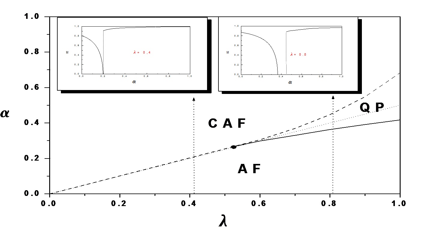
Figure 2: Ground state phase diagram in the $\lambda-\alpha$ plane for the quantum spin-$1/2$ $J_{1}-J_{1}^{\prime}-J_{2}$ model on a square lattice, where $\alpha=J_{2}/J_{1}$ and $\lambda=J_{1}^{\prime}/J_{1}$. The dashed and solid lines corresponds the first- and second-order transitions lines, respectively. The black point represents the quantum critical endpoint (QCE). The notations indicated by AF, CAF and QP corresponds the antiferromagnetic, collinear antiferromagnetic and quantum paramagnetic phases, respectively. The dotted line correspond the classical solution $\alpha_{c}=\lambda/2$.

V Conclusion

In summary, we have studied the effects of quantum fluctuations due to spatial ($\lambda$) and frustration ($\alpha$) parameter in the quantum spin-$1/2$ $J_{1}-J_{1}^{\prime}--J_{2}$ Heisenberg model. Using a variational method we calculated the sublattice magnetization for the AF and CAF phases. For values of $\lambda>0.51$ the frustration contributes significantly to the existence of a disordered intermediate state (QP) between the two AF and CAF ordered phases, while for $\lambda<0.51$, we have a direct first-order transition between the AF and CAF phases. We have observed, by analyzing the order parameters of the AF and CAF phases, that the phase transitions are of second and first-order between the AF-QP and CAF-QP, respectively. The obtained phase diagram can be compared with recent results which used effective-field theoryequivalence8 and coupled-cluster methodequivalence4 , showing the same qualitative results predicting a paramagnetic region for small interlayer parameter (i.e., $\lambda>\lambda_{1}$), and for $\lambda<\lambda_{1}$ this QP phase disappears by presenting a direct first-order transition between the AF and CAF phases. On the other hand, recent calculations of second order spin wave theoryequivalence7 have indicated that the intermediate QP phase exists for all $\lambda\leq 1$ in accordance with results of exact diagonalization12 . We speculate that by using a more sophisticated method, for example, quantum Monte Carlo simulationsmcq and density matrix renormalization group (DMRG) methoddmrg , this disordered region should disappear for certain values of $\lambda<\lambda_{1}$.

ACKNOWLEDGMENTS: This work was partially supported by CNPq (Brazilian agency)

References

- (1) Frustration Spin Systems, edited by H. T. Diep (World Scientific, Singapore, 2005).
- (2) Quantum Magnetism, Lectures Notes in Physics, No 645, edited by U. Schollwöck, J. Richter, D. J. J. Farnell, and R. F. Bishop (Springer-Verlag, Berlin, 2004).
- (3) P. Chandra and B. Doucot, Phys. Rev. B 38, 9335 (1988); see, also, L. B. Ioffe and A. I. Larkin, Mod. Phys. B 2, 203 (1988).
- (4) H. J. Schulz, T. A. L. Ziman, and D. Poiblanc, J. Phys. I France 6, 675 (1996); H. J. Schulz and T. A. L. Ziman, Europhys. Lett. 18, 355 (1992).
- (5) J. Richter, N. B. Ivanov, and K. Retzlaff, Europhys. Lett. 25, 545 (1994); N. B. Ivanov and J. Richter, J. Phys. Cond. Matter 6, 3785 (1994).
- (6) R. R. P. Singh, Zheng Weihong, C. J. Hamer, and J. Oitmaa, Phys. Rev. B 60, 7278 (1999).
- (7) L. Capriotti and S. Sorella, Phys. Rev. Lett. 84, 3173 (2000); L. Capriotti, A. Fubini, T. Roscilde, and V. Tognetti, Phys. Rev. Lett. 92, 157202 (2004).
- (8) C. Weber, F. Becca, and F. Mila, Phys. Rev. B 72, 24449 (2005).
- (9) L. Spanu and A. Parola, Phys. Rev. B 73, 944427 (2006); V. Lante and A. Parola, Phys. Rev. B 73, 94427 (2006).
- (10) R. Darradi, J. Richter, and D. J. J. Farnell, Phys. Rev. B 72, 104425 (2005).
- (11) J. Sirker, Zheng Weihong, O. O. Sushkov, and J. Oitmaa, Phys. Rev. B 73, 184420 (2006).
- (12) Ji-Feng Yu and Ying-Jer Kao, Phys. Rev. B 85, 094407 (2012).
- (13) P. Sindzingre, Phys. Rev. B 69, 94418 (2004).
- (14) R. F. Bishop, P. H. Y. Li, R. Darradi, J. Schulenburg, and J. Richter, Phys. Rev. B 78, 054412 (2008); R. F. Bishop, P. H. Y. Li, R. Darradi, J. Schulenburg, J. Richter, and C. E. Campbell, J. Phys.: Condens. Matter 20, 415213 (2008). See also, R. Darradi, J. Richter, J. Schulenburg, R. F. Bishop, and P. H. Y. Li, J. Phys.: Conference Series 145, 012049 (2009).
- (15) R. Darradi, O. Derzhko, R. Zinke, J. Schulenburg, S. E. Krüger, and J. Richter, Phys. Rev. B 78, 214415 (2008).
- (16) L. Isaev, G. Ortiz, and J. Dukelsky, Phys. Rev. B 79, 024409 (2009).
- (17) J. Roberto Viana and J. Ricardo de Sousa, Phys. Rev. B 75, 052403 (2007).
- (18) M. J. Oliveira, Phys. Rev. B 43, 6181 (1991).
- (19) J. Richter and J. Schulenburg, Eur. Phys. J B 73, 117 (2010).
- (20) R. Melzi, P. Carretta, A. Lascialfari, M. Mambrini, M. Troyer, P. Millet, and F. Mila, Phys. Rev. Lett. 85, 1318 (2000).
- (21) P. Carretta, R. Melzi, N. Papinutto, and P. Millet, Phys. Rev. Lett. 88, 047601 (2002); P. Carretta, N. Papinutto, C. B. Azzoni, M. C. Mozzati, E. Pavarini, S. Gonthier, and O. Millet, Phys. Rev. B. 66, 094420 (2002).
- (22) H. Rosner, R. R. P. Singh, Z. Weihong, J. Oitmaa, S. L. Drechsler, and W. Picket, Phys. Rev. Lett. 88, 18405 (2002).
- (23) A. Bombardi, J. Rodriguez-Carvajal, S. Di Matteo, F. de Bergevin, L. Paolasini, P. Carretta, P. Millet, and R. Caciuffo, Phys. Rev. Lett. 93, 027201 (2004).
- (24) F. Becca and F. Mila, Phys. Rev. Lett. 88, 067203 (2002).
- (25) E. Pavarini, S. C. Tarantino, T. Boffa Ballaran, M. Zema, P. Ghigna, and P. Carretta, Phys. Rev. B 77, 014425 (2008).
- (26) A. A. Nersesyan and A. M. Tsvelik, Phys. Rev. B 67, 024422 (2003).
- (27) O. A. Starykh and L. Balent, Phys. Rev. Lett. 93, 127202 (2004).
- (28) P. Sindzingre, Phys. Rev. B 69, 094418 (2004).
- (29) J. I. Igarashi and T. Nagao, Phys. Rev. B 72, 014403 (2005).
- (30) R. F. Bishop, P. H. Y. Li, R. Darradi, and J. Richter, J. Phys.: Cond. Matter 20, 255251 (2008).
- (31) H. C. Jiang, F. Krüger, J. E. Moore, D. N. Sheng, J. Zaanen, and Z. Y. Weng, Phys. Rev. B 79, 174409 (2009).
- (32) Alexander A. Tsirlin and H. Rosner, Phys. Rev. B 79, 214417 (2009).
- (33) K. Majumdar, Phys. Rev. B 82, 144407 (2010). See also, K. Majumdar, D. Furton, and G. S. Uhrig, Phys. Rev. B 85, 144420 (2012).
- (34) G. Mendonça, Rodrigo S. Lapa, Minos A. Neto, J. Ricardo de Sousa, K. Majumdar, and T. Datta, J. Stat. Mech., P06022 (2010).
- (35) E. H. Büchmer, Z. Phys. Chem. 56, 257 (1906).
- (36) M. E. Fisher and P. J. Upton, Phys. Rev. Lett. 65, 2402 (1990); ibid 65, 3405 (1990).
- (37) M. E. Fisher and M. C. Barbosa, Phys. Rev. B 43, 11177 (1991); M. C. Barbosa and M. E. Fisher, Phys. Rev. B 43, 10635 (1991); M. C. Barbosa, Phys. Rev. B 45, 5199 (1992).
- (38) E. Manousakis, Rev. Mod. Phys. 63, 1 (1991).
- (39) H. W. de Wijn, R. E. Walstedt, L. R. Walker, and H. J. Guggenheim, Phys. Rev. Lett. 24, 832 (1970).
- (40) R. E. Walstedt, H. W. de Wijn, and H. J. Guggenheim, Phys. Rev. Lett. 25, 119 (1970).
- (41) R. Coldea, S. M. Hayden, G. Aeppli, T. G. Perring, C. D. Frost, T. E. Mason, S. -W. Cheong, and Z. Fisk, Phys. Rev. Lett. 86, 5377 (2001).
- (42) A. W. Sandvik, Phys. Rev. B 56, 11678 (1997).
- (43) H. C. Jiang, H. Yao, and L. Balents, Cond. mat. arXiv:1112.224 (2011).