“Counterpart” method for abundance determinations in H II regions

Abstract

We suggest a new way of the determining abundances and electron temperatures in H ii regions from strong emission lines. Our approach is based on the standard assumption that H ii regions with similar intensities of strong emission lines have similar physical properties and abundances. A “counterpart” for a studied H ii region may be chosen among H ii regions with well-measured abundances (reference H ii regions) by comparison of carefully chosen combinations of strong line intensities. Then the abundances in the investigated H ii region can be assumed to be the same as those in its counterpart. In other words, we suggest to determine the abundances in H ii regions “by precedent”. To get more reliable abundances for the considered H ii region, a number of reference H ii regions is selected and then the abundances in the target H ii region are estimated through extra-/interpolation. We will refer to this method of abundance determination as the counterpart method or, for brevity, the $C$ method. We define a sample of reference H ii regions and verify the validity of the $C$ method. We find that this method produces reliable abundances. Finally, the $C$ method is used to obtain the radial abundance distributions in the extended discs of the spiral galaxies M 83, NGC 4625 and NGC 628.

1 Introduction

Metallicities play a key role in many studies of galaxies. While absorption line indices are widely used to derive the metallicities of older stellar populations, gas-phase oxygen abundances are the best means to estimate the present-day metallicities. Since emission lines in the spectra of H ii regions are easily measurable across a wide range of extragalactic distances, they are generally considered the most powerful indicators of the present-day chemical composition of star-forming galaxies. The spectra of a large number of individual H ii regions in nearby spiral and irregular galaxies have now been obtained (see McCall et al., 1985; Zaritsky et al., 1994; van Zee et al., 1998; van Zee & Haynes, 2006; Izotov et al., 1997; Izotov & Thuan, 1998b, 2004; Kehrig et al., 2004; Bresolin et al., 1999, 2005, 2009a, 2009b; López-Sánchez & Esteban, 2009; Guseva et al., 2011, among many others). These spectroscopic measurements provide the basis for investigations of metallicity properties of galaxies such as radial abundance gradients, mean metallicities, etc., (Vila-Costas & Edmunds, 1992; Zaritsky et al., 1994; van Zee et al., 1998; Pilyugin et al., 2004, among others).

The H ii regions ionised by stars (or star clusters) form a well-defined fundamental sequence in different emission-line diagrams. The existence of such a fundamental sequence provides the basis of various investigations of extragalactic H ii regions. In particular, Baldwin, Phillips & Terlevich (1981) suggested that the position of an object in some well-chosen emission-line diagrams can be used to separate H ii regions ionised by stars from other types of emission-line objects. This idea has found general acceptance and is widely used. Thus, the [O iii]$\lambda$5007/H${\beta}$ vs. [N ii]$\lambda$6584/H${\alpha}$ diagram is often used to distinguish between H ii regions and active galactic nuclei (AGNs). However, the exact location of the dividing line between H ii regions and AGNs is still controversial (Kewley et al., 2001; Kauffmann et al., 2003; Stasińska et al., 2006). It has been argued that the binary classification scheme for emission line galaxies (subdividing into star-forming galaxies and AGNs) is oversimplified and a revised classification scheme involving more classes should be considered (Stasińska et al., 2008; Cid Fernandes et al., 2011).

Pagel et al. (1979) and Alloin et al. (1979) suggested that the positions of H ii regions in some emission-line diagrams can be calibrated in terms of their oxygen abundances. This approach to abundance determination in H ii regions, usually referred to as the “strong-line method” or “strong-line calibrations” has been widely adopted. Numerous relations have been suggested to convert metallicity-sensitive emission-line ratios into metallicity or temperature estimates (Dopita & Evans, 1986; McGaugh, 1991; Zaritsky et al., 1994; Pilyugin, 2000, 2001; Kewley & Dopita, 2002; Pilyugin & Thuan, 2005; Pettini & Pagel, 2004; Tremonti et al., 2004; Stasińska, 2006, among many others).

It should be stressed that strong-line calibrations for oxygen abundances do not form a uniform ”family”. Basically, there are two types. The calibrations of the first type are the empirical calibrations, established on the basis of H ii regions in which the oxygen abundances are determined through the $T_{e}$ method. The calibrations of the second type are the theoretical (or model) calibrations, established on the basis of grids of photoionisation models of H ii regions. Among published strong-line calibrations there exist large systematic discrepancies, in the sense that theoretical calibrations generally produce oxygen abundances that are by factors of 1.5 – 5 higher than those derived using empirical calibrations (c.f. Kennicutt et al., 2003; Pilyugin, 2003b; Yin et al., 2007; Kewley & Ellison, 2008; Bresolin et al., 2009b; Moustakas et al., 2010; López-Sánchez & Esteban, 2010). Thus, at the present time there exists no absolute scale for metallicities in H ii regions.

The empirical metallicity scale has advantages as compared to the theoretical (model) metallicity scales. The empirical metallicity scale is well defined in terms of the abundances in H ii regions derived through the $T_{e}$ method, i.e., in that sense the empirical metallicity scale is absolute. The abundances estimated via different empirical calibrations are compatible with each other and with the $T_{e}$-based abundances as well. Contrary to the consistency among empirical calibrations, there are as many theoretical (model) metallicity scales as there are sets of H ii region models. In other words, the abundances derived using different theoretical calibrations are usually not in agreement with each other. However, the validity of the $T_{e}$ method (and, as a consequence, the validity of the empirical metallicity scale in H ii regions) has for long been questioned (Peimbert, 1967; Stasińska, 2005; Peña-Guerrero et al., 2012, and references therein). But there is also evidence that the classic $T_{e}$ method provides realistic oxygen abundances of H ii regions (Pilyugin, 2003b; Pilyugin et al., 2006; Williams et al., 2008; Bresolin et al., 2009b; Rodríguez & García-Rojas, 2010). It is also noteworthy that oxygen abundances in Galactic H ii regions derived using the direct $T_{e}$ method as well as empirical calibrations agree with stellar oxygen abundances (see, e.g., Fig. 7 in Mattsson, 2010) determined in Cepheids (Andrievsky et al., 2002a, b, c, 2004) as well as the new solar oxygen abundance (Asplund et al., 2009). Moreover, if the empirical metallicity scale should be corrected (see, e.g. Peña-Guerrero et al., 2012), the abundances derived using the $T_{e}$ method and different empirical calibrations should be corrected accordingly. Thus, the empirical metallicity scale is likely the preferable metallicity scale at present.

However, all calibrations (empirical as well as theoretical) encounter problems. These calibrations are usually based on the oxygen [O ii]$\lambda$3727+$\lambda$3729, [O iii]$\lambda$5007 and/or nitrogen [N ii]$\lambda$6584 lines [with a few exceptions, e.g., Stasińska (2006)]. It is well known that the relation between the oxygen abundance and the strong oxygen-line intensities is double-valued, with two distinct parts, traditionally known as the upper (12 + log(O/H) $\ga$ 8.25) and lower (12 + log(O/H) $\la$ 8.0) branches of the R₂₃ – O/H diagram. Moreover, the strong oxygen-line intensities are not a good indicator of the oxygen abundance in the transition zone between the upper and lower branches.

Furthermore, it is well known that there is no one-to-one correspondence between oxygen and nitrogen abundances. A prominent feature of the N/O vs. O/H diagram is that the N/O abundance ratio shows a large scatter at a fixed value of the O/H abundance ratio, larger than can be explained by observational uncertainties (Henry et al., 2000; Pilyugin et al., 2003; López-Sánchez & Esteban, 2010). The N/O – O/H relation shows also a clear bend: while at low metallicities (12 +log(O/H) $\la$ 8.0) the N/O abundance ratio is, on average, constant, the N/O ratio increases with O/H at high metallicities (12 +log(O/H) $\ga$ 8.0).

The properties mentioned above prevent the construction of a calibration that works over the whole range of metallicities shown by H ii regions. Thus, one has to construct separate calibrations for different metallicity intervals, i.e., there are no calibration relations that work sufficiently well over the whole range of observed metallicities. Here, also another problem arises – one has to know a priori in which metallicity interval (or on which of the two branches) the H ii region is located.

It should be emphasised that each existing calibration is based on the assumption that H ii regions with similar strong-line intensities have similar abundances. A simple, more direct method for abundance determination follows from that assumption as well. If there were (and fortunately there is indeed) a suitable sample of reference H ii regions with well-measured electron temperatures and abundances, then one can choose among those reference H ii regions the ones that have the smallest difference in strong line intensities compared to the studied H ii region, i.e., one can find a corresponding, “counterpart” H ii region. Then the oxygen and nitrogen abundances and electron temperatures in the investigated H ii region can be assumed to be the same as in its counterpart. In other words, we suggest that the abundances in the target H ii region can be determined “by precedent”. To obtain more reliable abundances, one may select several reference H ii regions (counterparts) and then estimate the abundance in the target H ii region through extrapolation or interpolation. We will refer to this method as the “counterpart method” or, for brevity, as the $C$ method.

The main goal of the present study is to select a sample of H ii regions with well-measured electron temperatures and abundances, i.e., to obtain a sample of reference H ii regions. We have carried out an extensive search of the literature to compile a list of spectra of H ii regions in irregular and spiral galaxies with measured electron temperatures. The sample of reference H ii regions and the $C$ method are discussed in Section 2. In Section 3, the $C$ method is used to obtain abundance gradients in the extended discs of three spiral galaxies. Section 4 presents the conclusions.

Throughout the paper, we will use the following standard notations for the line intensities:
$R$ = $I_{\rm[O\,III]\lambda 4363}/I_{{\rm H}\beta}$,
$R_{2}$ = $I_{\rm[O\,II]\lambda 3727+\lambda 3729}/I_{{\rm H}\beta}$,
$N_{2}$ = $I_{\rm[N\,II]\lambda 6548+\lambda 6584}/I_{{\rm H}\beta}$,
$S_{2}$ = $I_{\rm[S\,II]\lambda 6717+\lambda 6731}/I_{{\rm H}\beta}$,
$R_{3}$ = $I_{{\rm[O\,III]}\lambda 4959+\lambda 5007}/I_{{\rm H}\beta}$.
$S_{3}$ = $I_{{\rm[S\,III]}\lambda 9068+\lambda 9532}/I_{{\rm H}\beta}$.
The electron temperatures will be given in units of 10⁴K.

2 A sample of reference H ii regions

2.1 Observational data: line intensities

We have carried out an extensive search of the literature and compiled a sample of H ii regions with abundances determined with the $T_{e}$ method. This sample is the basis for our study. We have searched for spectra of H ii regions in irregular and spiral galaxies, with the requirement that they include the [O ii]$\lambda$3727+$\lambda$3729, [O iii]$\lambda$5007, [N ii]$\lambda$6584, [S ii]$\lambda$6717+$\lambda$6731 lines and a detected auroral line of, at least, one ion, i.e., [O iii], [N ii], [S iii]. The electron temperature $t_{2}$ in H ii regions can also be estimated from the [O ii]$\lambda$$\lambda$3727,3729/[O ii]$\lambda$$\lambda$7320,7330 ratio. However, the difference between the $t_{2}$ temperature derived from the [O ii]$\lambda$$\lambda$3727,3729/[O ii]$\lambda$$\lambda$7320,7330 ratio and the one estimated from the commonly used $t_{2}$ – $t_{3}$ relation can be large (see the discussion in Kennicutt et al. (2003) and references therein), making the oxygen abundances so derived very uncertain. Therefore, H ii regions with a temperature derived from the [O ii]$\lambda$$\lambda$3727,3729/[O ii]$\lambda$$\lambda$7320,7330 ratio are not considered in the present study. While we have tried to include as many sources as possible, we do not claim our search to be exhaustive.

In recent years, the number of available spectra of emission-line nebulae has increased dramatically due to several large spectroscopic surveys such as the Sloan Digital Sky Survey (SDSS) (York et al., 2000). The auroral lines are measurable in a relatively large number of SDSS galaxies (Kniazev et al., 2004; Izotov et al., 2006), which provides the possibility to obtain $T_{e}$-based abundances for SDSS galaxies. However, the SDSS objects cannot be used as reference H ii regions for two reasons. First, the wavelength range of the SDSS spectra is 3800 – 9300 Å so that for nearby galaxies with redshift $z\la 0.02$ the [O ii]$\lambda$3727+$\lambda$3729 emission line is outside of that range. The lack of this line prevents us from using SDSS spectra of nearby galaxies in our study. Second, the SDSS galaxy spectra span a large range of redshifts. There is thus an aperture-redshift effect in SDSS spectra since these spectra are obtained with $3^{\prime\prime}$-diameter fibers. At a redshift of $z=0.05$ the projected aperture diameter is $\sim$ 3 kpc, while it is $\sim$ 15 kpc at a redshift of $z=0.25$. This means that, at large redshifts, SDSS spectra are closer to global spectra of whole galaxies, i.e., to spectra of composite nebulae including multiple star clusters, rather than to spectra of individual H ii regions. It has been argued that the $T_{e}$ method can result in an underestimated oxygen abundance in the SDSS objects if H ii regions with different physical properties contribute to the global spectrum of composite nebulae (Pilyugin et al., 2012). This effect is somewhat similar to the small-scale temperature fluctuations in H ii regions discussed by Peimbert (1967).

High-precision spectroscopy, including the auroral lines [O iii]$\lambda$4363 and [N ii]$\lambda$5755 for a number of H ii regions in our Galaxy (see Esteban et al., 2004; García-Rojas et al., 2004, 2005, 2006; García-Rojas & Esteban, 2007, among others) and in the Large and Small Magellanic Clouds (e.g. Peimbert, 2003; Tsamis et al., 2003; Peimbert et al., 2005; Peña-Guerrero et al., 2012) can be found in the literature. However, only a small part of the H ii regions is measured in these cases and therefore the obtained line intensities are usually not representative for the whole nebula. For this reason, these spectroscopic measurements were not included in our list.

Thus, for each listed spectrum, we record the measured values of [O ii]$\lambda$3727+$\lambda$3729, [O iii]$\lambda$4363, [O iii]$\lambda$5007, [N ii]$\lambda$5755, [S iii]$\lambda$6312, [N ii]$\lambda$6584, [S ii]$\lambda$6717+$\lambda$6731, [S iii]$\lambda$9068. The intensities of all lines are normalised to the H$\beta$ line flux. The line intensity [O iii]$\lambda$4959 is required to define the $R_{3}$ value. However this line is not reported in some of the papers considered here. Therefore the $R_{3}$ value is derived from the [O iii]$\lambda$5007 line intensity (see below). Similarly, the values of $N_{2}$ and $S_{3}$ are estimated without the lines [N ii]$\lambda$6548 and [S iii]$\lambda$9532, which are also not reported in some papers. Furthermore, only the summed-up line fluxes [S ii]$\lambda$6717+$\lambda$6731 are available in a number of publications.

We have taken the de-reddened line intensities as reported by the authors. In some papers the measured fluxes are reported only. In these cases, the measured emission-line fluxes were corrected for interstellar reddening using the theoretical H$\alpha$ to H$\beta$ ratio (i.e., the standard value of H$\alpha$/H$\beta$ = 2.86) and the analytical approximation to the Whitford interstellar reddening law from Izotov et al. (1994).

As was noted above, only one line in a doublet ([O iii]$\lambda$5007 from the doublet [O iii]$\lambda$5007 + $\lambda$4959, [N ii]$\lambda$6584 from the doublet [N ii]$\lambda$6584 + $\lambda$6548, and [S iii]$\lambda$9068 from the doublet [S iii]$\lambda$9068 + $\lambda$9532) is given in some publications. The [O iii]$\lambda$5007 and $\lambda$4959 lines originate from transitions from the same energy level, so their flux ratio is due only to the transition probability ratio, which is very close to 3 (Storey & Zeippen, 2000). Therefore, the value of $R_{3}$ can be estimated as $R_{3}=1.33$[O iii]$\lambda$5007. Similarly, the [N ii]$\lambda$6584 and $\lambda$6548 lines also originate from transitions from the same energy level and the transition probability ratio for those lines is again close to 3 (Storey & Zeippen, 2000). The value of $N_{2}$ can therefore be estimated as $N_{2}$ = 1.33[N ii]$\lambda$6584. Furthermore, the transition probability ratio for [S iii]$\lambda$9532 and [S iii]$\lambda$9068 is 2.44 (Mendoza & Zeippen, 1982). Hence, the value of $S_{3}$ can be estimated as $S_{3}$ = 3.44[S iii]$\lambda$9068.

The spectroscopic data so assembled form the basis of the present study. Our list contains 714 spectra. Since two or three auroral lines are detected in some spectra the resulting number of electron temperatures measurements is 899 (645 measurements of $t_{3,O}$ electron temperatures, 140 measurements of $t_{2,N}$ electron temperatures, and 114 measurements of $t_{3,S}$ electron temperatures).

2.2 Abundance derivation

In principle, the T_e method, based on measurements of temperature-sensitive line ratios, should give accurate oxygen abundances. In practice, however, oxygen abundances in the same H ii region derived by various authors can differ because there may be errors in the line intensity measurements and the adopted atomic data may not be the same. To ensure that we have a relatively homogeneous data set, we have recalculated electron temperatures and oxygen and nitrogen abundances for all the H ii regions.

To convert the values of the line fluxes to the electron temperatures $t_{\rm 3,O}$, $t_{\rm 2,N}$, and $t_{\rm 3,S}$ and to the ion abundances O⁺⁺/H⁺, O⁺/H⁺, and N⁺/H⁺, we have solved the five-level atom model for the O⁺⁺, O⁺, N⁺, and S⁺⁺ ions, using recent atomic data. The Einstein coefficients for the spontaneous transitions $A_{jk}$ for the five low-lying levels for all ions above have been taken from Froese Fisher & Tachiev (2004). The energy level data are from Edlén (1985) for O⁺⁺, from Wenåker (1990) for O⁺, from Galavís et al. (1997) for N⁺, and from Johansson et al. (1992) for S⁺⁺. The effective cross sections (or effective collision strengths) for electron impact $\Omega$_jk as a function of temperature are from Aggarwal & Keenan (1999) for O⁺⁺, from Pradhan et al. (2006) for O⁺, from Hudson & Bell (2005) for N⁺, and from Tayal & Gupta (1999) for S⁺⁺. To derive the effective cross section for a given electron temperature, we have fitted a second-order polynomial to these data.

In the low density regime ($n_{e}\la 100$ cm^-3), the following simple expressions provide approximations to the numerical results with an accuracy better than 1%. The electron temperatures are related to the measured line fluxes in the following way:

$$t_{\rm 3,O}=\frac{1.467}{\log Q_{\rm 3,O}-0.876-0.193\log t_{\rm 3,O}+0.033\,t_{\rm 3,O}}$$ (1)

and

$$t_{\rm 2,N}=\frac{1.118}{\log Q_{\rm 2,N}-0.891-0.177\log t_{\rm 2,N}+0.030\,t_{\rm 2,N}}$$ (2)

or

$$t_{\rm 3,S}=\frac{0.915}{\log Q_{\rm 3,S}-0.683+0.485\log t_{\rm 3,S}-0.114\,t_{\rm 3,S}}$$ (3)

where $Q_{\rm 3,O}$ = [O iii]($\lambda$4959+$\lambda$5007)/[O iii]$\lambda 4363$ is the ratio of nebular to auroral oxygen O⁺⁺ line intensities, $Q_{\rm 2,N}$ = [N ii]($\lambda 6548+\lambda 6584$)/[N ii]$\lambda 5755$ is the ratio of nebular to auroral nitrogen N⁺ line intensities, and $Q_{\rm 3,S}$ = [S iii]($\lambda 9068+\lambda 9532$)/[S iii]$\lambda$ 6312 is the ratio of nebular to auroral sulphur S⁺⁺ line intensities.

The equations relating ion abundances to measured line fluxes are:

$$12+\log\frac{\rm N^{+}}{\rm H^{+}}=\log N_{2}+6.263+\frac{0.893}{t_{2}}-0.603\,\log t_{2}-0.003\,t_{2},$$ (4)

$$12+\log\frac{\rm O^{+}}{\rm H^{+}}=\log R_{2}+5.929+\frac{1.617}{t_{2}}-0.568\,\log t_{2}-0.008\,t_{2},$$ (5)

and

$$12+\log\frac{\rm O^{++}}{\rm H^{+}}=\log R_{3}+6.251+\frac{1.204}{t_{3}}-0.613\,\log t_{3}-0.015\,t_{3}.$$ (6)

The total oxygen abundance is determined from

$$\frac{\rm O}{\rm H}=\frac{\rm O^{++}}{\rm H^{+}}+\frac{\rm O^{+}}{\rm H^{+}}.$$ (7)

In general, the small fraction of undetected O³⁺ ions in the high-excitation H ii regions (O⁺/(O⁺+O²⁺) $<$ 0.1) should be added to the oxygen abundance (Izotov et al., 2006). However, this results in only a minor correction to the oxygen abundance derived just from O⁺ and O²⁺. For example, the correction is around 0.01 dex for the lowest-metallicity blue compact dwarf galaxy SBS 0335-052 (Izotov et al., 2009). Hence, this correction is not considered in the following.

The total nitrogen abundance is determined from

$$\log\frac{\rm N}{\rm H}=\log\frac{\rm O}{\rm H}+\log\frac{\rm N}{\rm O}$$ (8)

assuming (Peimbert & Costero, 1969)

$$\frac{\rm N^{+}}{\rm O^{+}}=\frac{\rm N}{\rm O}.$$ (9)

The N⁺/O⁺ ion abundance ratio is derived from

$$\log\frac{\rm N^{+}}{\rm O^{+}}=\log\frac{\rm N_{2}}{\rm R_{2}}+0.334-\frac{0.724}{t_{2}}-0.035\log t_{2}+0.005t_{2}$$ (10)

which is obtained by combining Eq.(4) with Eq.(5).

We have calculated electron temperatures and oxygen and nitrogen abundances for H ii regions within the framework of the standard H ii region model with two distinct temperature zones within the nebula. The electron temperature $t_{3}$ within the zone O⁺⁺ is given by the electron temperature $t_{3,O}$, and the temperature $t_{2}$ within the zones O⁺ and N⁺ is given by the temperature $t_{2,N}$. It is common practice that the value of only the electron temperature is measured and the value of the other temperature is determined from the $t_{2}$ – $t_{3}$ relation. The commonly used $t_{2}$ – $t_{3}$ relation (Campbell et al., 1986; Garnett, 1992)

$$t_{2}=0.7\,t_{3}+0.3$$ (11)

is adopted here. When the value of the electron temperature $t_{3,S}$ is measured then the value of $t_{3}$ is obtained from the relation after Garnett (1992)

$$t_{3}=0.83\,t_{3,S}+0.17.$$ (12)

Two or three auroral lines are detected in some spectra and, consequently, two or three electron temperatures ($t_{3,O}$, $t_{2,N}$, $t_{3,S}$) can be measured. For those H ii regions, two or three values of the electron temperature $t_{3}$ and oxygen and nitrogen abundances are determined.

2.3 The $C$ method

Suppose we have an observed H ii region and a sample of reference H ii regions. To find the counterpart for the H ii region under study, we will compare not the four measured nebular lines $R_{3}$, $R_{2}$, $N_{2}$, and $S_{2}$ directly, but instead four other values that are expressed in terms of these line intensities: $P$ = $R_{3}$/($R_{2}$ + $R_{3}$) (excitation parameter), log$R_{3}$, log($N_{2}$/$R_{2}$), and log($S_{2}$/$R_{2}$). A linear combination of these values can serve as an indicator of the metallicity in an H ii region (Pilyugin et al., 2010).

We specify the difference between the spectrum of the studied H ii region and the spectrum of the $j$th H ii region from the reference sample as

$$\begin{array}[]{lll}\Delta{\rm Sp}_{j}&=&[\frac{1}{4}((\Delta\log(R_{3})_{j})^{2}+(\Delta P_{j})^{2}\\ &+&(\Delta\log(N_{2}/R_{2})_{j})^{2}+(\Delta\log(S_{2}/R_{2})_{j})^{2})]^{\frac{1}{2}}.\\ \end{array}$$ (15)

The reference H ii region with the smallest value of the $\Delta$Sp will be considered as the counterpart for the investigated H ii region. Then the oxygen and nitrogen abundances and electron temperature in the studied H ii region can be assumed to be the same as those in its counterpart.

However, oxygen and nitrogen abundances obtained in this manner can still have considerable errors for the following reasons.
1. The number of reference H ii regions is limited, especially at the high-metallicity end. Hence, in some cases there may be significant differences between abundances of the studied H ii region and its counterpart.
2. In some cases the smallest value of $\Delta$Sp does not corresponds to the minimum difference in oxygen abundance. That would be the case if all the values of $P$, log$R_{3}$, log($N_{2}$/$R_{2}$), and log($S_{2}$/$R_{2}$) would change in proportion to the change of the abundance, and the calibration coefficients would be the same for all those values. This is indeed not the case. The coefficients are in fact functions of the metallicity (for example, the coefficient for log$R_{3}$ even changes sign going from low-metallicity to high-metallicity H ii regions). Furthermore, the difference in log($N_{2}$/$R_{2}$) values between two H ii regions with the same oxygen abundance but different N/O abundance ratios can be larger than the difference between two H ii regions with different oxygen abundances but similar nitrogen abundances. Thus, one may assume that the reference H ii region with the smallest value of the $\Delta$Sp has a similar, but not necessarily the abundance closest to that of the studied H ii region.
3. Finally, the $T_{e}$-based abundances for the reference H ii region can of course involve some errors and uncertainties.

To overcome these problems and obtain more reliable estimates of abundances and electron temperatures, a number of reference H ii regions with metallicities near the metallicity of the selected counterpart H ii region, (in the metallicity interval $\pm$(O/H)_int) can be used. Using a sufficient number of H ii regions with metallicities in a suitable interval, one can obtain a linear expression for the oxygen abundance (or nitrogen abundance and electron temperature) of the form

$$Y=a_{0}+a_{1}\log R_{3}+a_{2}P+a_{3}\log(N_{2}/R_{2})+a_{4}\log(S_{2}/R_{2}),$$ (16)

where $Y=12+\log$(O/H), or $Y=12+\log$(N/H), or $Y=t_{3}$. The oxygen and nitrogen abundances determined this way will in the following be referred to as (O/H)_C and (N/H)_C, respectively.

2.4 Selection of the reference H ii regions

The selection of reference H ii regions is not a trivial task. Here we use an approach that is based on the idea that if an H ii region belongs to the fundamental sequence of the photoionised nebulae, and its line fluxes are measured accurately, then the different methods, based on different emission lines, should yield similar physical characteristics (such as electron temperatures and abundances) of that object (Thuan et al., 2010).

The $C$ method requires we first select a sample of reference H ii regions from the collected data. The uncertainty of the oxygen abundance can be quantified by the discrepancy between the $C$-based and the $T_{e}$-based oxygen abundances $D_{O/H}$ = (O/H)_C – (O/H)${}_{T_{e}}$. Similarly, the uncertainty in the nitrogen abundance can be quantified by $D_{N/H}$ = (N/H)_C – (N/H)${}_{T_{e}}$. One may select reference H ii regions where the discrepancies in the oxygen and nitrogen abundances are less than a fixed value of $D_{O/H}^{*}$ and $D_{N/H}^{*}$. We use an iterative procedure to select a sample of reference H ii regions. In the first step, we determine the oxygen (O/H)_C and nitrogen (N/H)_C abundances from Eq. (16) for each H ii region in our list using all the other H ii regions as the reference sample. Then we select a subsample of H ii regions for which the absolute difference between the $C$-based and the $T_{e}$-based abundances (O/H)_C – (O/H)${}_{T_{e}}$ is less than $D_{O/H}^{*}$ and the absolute difference (N/H)_C – (N/H)${}_{T_{e}}$ is less than $D_{N/H}^{*}$. In the second step, we again determine oxygen (O/H)_C and nitrogen (N/H)_C abundances from Eq. (16) for each H ii region in our list using a selected subsample of H ii regions as the reference sample. We then select a new subsample of H ii regions for which the difference between $C$-based and $T_{e}$-based abundances is less than $D_{O/H}^{*}$ and $D_{N/H}^{*}$, i.e., a new sample of reference H ii regions is obtained. The algorithm converges after a number (around ten) of iterations. As was noted above, two or three auroral lines are detected in some spectra and, consequently, two or three electron temperatures ($t_{3,O}$, $t_{2,N}$, $t_{3,S}$) can be measured. For those H ii regions more than one (i.e., two or three) oxygen and nitrogen abundances are determined. If these abundances, for a given spectrum, satisfy the selection criteria, we choose that one for which the difference between $C$-based and $T_{e}$-based oxygen abundances is the smallest.

In general, the selected sample of reference H ii regions depends on three parameters:
1) the adopted interval of metallicity around the metallicity of the counterpart (O/H)_int which defines a subsample of reference H ii regions used to derive the coefficients in Eq. (16),
2) the adopted maximum value of $D_{O/H}^{*}$, i.e., of the discrepancy between $C$-based and $T_{e}$-based oxygen abundances in the reference H ii regions,
3) the adopted maximum value of $D_{N/H}^{*}$, i.e., of the discrepancy between $C$-based and $T_{e}$-based nitrogen abundances in the reference H ii regions.

Examining the samples of reference H ii regions selected with different combinations of the values of $D_{O/H}^{*}$ (from an interval of 0.06 – 0.12 dex), $D_{N/H}^{*}$ (from an interval of 0.06 – 0.12 dex) and (O/H)_int (from an interval of 0.15 – 0.30 dex), we find that oxygen and nitrogen abundances obtained by the $C$ method with $D_{O/H}^{*}$ in the range 0.08 to 0.12 dex, $D_{N/H}^{*}=$ 0.08 to 0.12 dex, and (O/H)${}_{int}=$ 0.20 to 0.30 dex are very similar.

Therefore we will discuss below only three samples of the reference H ii regions from the sequence defined by $D_{N/H}^{*}=D_{O/H}^{*}$ and (O/H)${}_{int}=2D_{O/H}^{*}$. In this case each sample of reference H ii regions can be specified by a single parameter, $D_{O/H}^{*}$. The sample with $D_{O/H}^{*}=0.12$ dex has been selected from our compilation of H ii regions in the way described above. If the number of reference H ii regions within the adopted interval of metallicity around the metallicity of the counterpart (O/H)_int, which defines a subsample of reference H ii regions used to derive the coefficients in Eq.(16), is less than 12 (this can occur at the high-metallicity end) then we increase the interval of metallicity (O/H)_int with a step size of 0.05 dex until the number of reference H ii regions within the adopted interval of metallicity becomes larger than 12. This sample will be referred to as $Rsample12$ below. In a similar way the sample $Rsample10$ with $D_{O/H}^{*}$ = 0.10 dex was selected from the sample $Rsample12$, and the sample $Rsample08$ with $D_{O/H}^{*}$ = 0.08 dex was selected from the sample $Rsample10$.

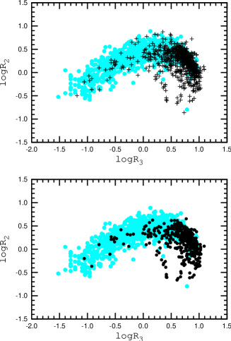
Figure 1: The log$R_{3}$ – log$R_{2}$ diagram. The filled grey (light-blue in the color version) circles in both panels are H ii regions from the compilation by Pilyugin et al. (2004). The dark (black) plus signs in the upper panel are H ii regions from our present compilation. The filled dark (black) circles in the lower panel show the selected reference H ii regions, $Rsample10$. (A color version of this figure is available in the online version.)

Figure 2: The solid line shows the cumulative number of individual oxygen abundance measurements of H ii regions with the absolute value of the difference between the $C$-based and the $T_{e}$-based abundances (discrepancy index $D_{\rm O/H}$) less than a given value. The dashed line is the same but for nitrogen abundance.

We choose $Rsample10$ for our abundance derivation. $Rsample12$ and $Rsample08$ will be used below to illustrate that the $C$-method abundances are robust. The reference H ii regions from the $Rsample10$ are listed in Table 1. Column 1 in the Table 1 is the order number of the H ii region. The de-reddened line intensities (in units of H$\beta$ line flux) are given in columns 2 to 5. $T_{e}$-based oxygen and nitrogen abundances [in units of 12+log(X/H)] are listed in columns 6 and 7 respectively, and the electron temperature (in units of 10⁴ K) is reported in column 8. In all cases where the electron temperature was reduced to $t_{3,O}$ [Eq. (11) or Eq. (12)] this is mentioned. The index $j_{T}$ in column 9 is equal to 1 when the electron temperature $t_{3,O}$ is derived from the auroral line [O iii]$\lambda$4363, equal to 2 when the temperature $t_{2,N}$ is derived from the auroral line [N ii]$\lambda$5755, and equal to 3 when the temperature $t_{3,S}$ is derived from the auroral line [S iii]$\lambda$6312. Commonly used catalogue names for each H ii region and the sources of the spectral data are listed in columns 10 and 11, respectively.

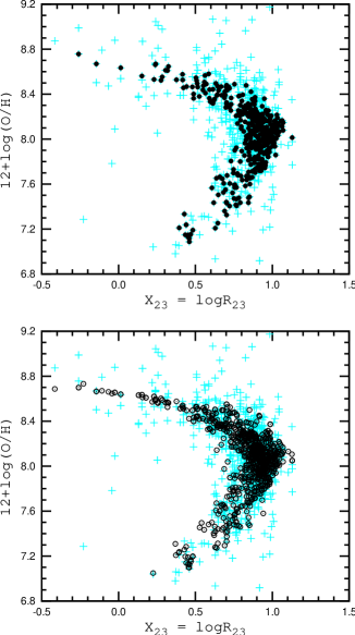
Figure 3: The log$R_{23}$ – O/H diagram. The grey (light-blue) plus signs in both panels are H ii regions from our present compilation for the case of the $T_{e}$-based abundances. The dark (black) filled circles in the upper panel show the selected reference H ii regions, $Rsample10$. The open dark (black) circles in the lower panel the H ii regions from the present compilation for the case of the $C$-based oxygen abundances. (A color version of this figure is available in the online version.)

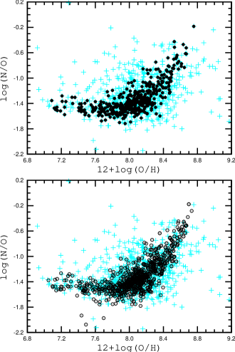
Figure 4: The O/H – N/O diagram. The grey (light-blue) plus signs in both panels are H ii regions from our present compilation for the case of the $T_{e}$-based abundances. The dark (black) filled circles in the upper panel show the selected reference H ii regions, $Rsample10$. The open dark (black) circles in the lower panel are the H ii regions from the present compilation for the case of the $C$-based oxygen abundances. (A color version of this figure is available in the online version.)

Let us briefly consider the general properties of $Rsample10$. Fig. 1 shows the log$R_{3}$ vs. log$R_{2}$ diagram. Pilyugin et al. (2004) compiled a large number of strong emission line measurements in spectra of individual H ii regions in nearby spiral and irregular galaxies. Those H ii regions are shown by filled gray (light-blue in the color version) circles in Fig. 1 (both panels) in order to outline the area occupied by H ii regions of nearby galaxies in the $R_{3}$ vs.  $R_{2}$ diagram. The H ii regions from the present compilation are shown by the dark (black) plus signs in the upper panel of Fig. 1. The selected reference H ii regions are shown by filled dark (black) circles in the lower panel of Fig. 1.

The solid line in Fig. 2 shows the cumulative number of individual oxygen abundance measurements from our compilation of H ii regions with the absolute difference between the $C$-based and the $T_{e}$-based oxygen abundances (discrepancy index D_O/H) less than a given value. The dashed line shows the same for the nitrogen abundances. One can clearly see that the cumulative numbers of nitrogen abundance measurements at any discrepancy index is larger than that for oxygen abundances, i.e., agreement between the $C$-based and the $T_{e}$-based abundances is better for nitrogen than for oxygen abundances.

Fig. 3 shows the log$R_{23}$ vs. O/H diagram. The $T_{e}$-based oxygen abundances for H ii regions from our compilation are indicated by the grey (light-blue) plus signs in both panels of Fig. 3. The log$R_{23}$ vs. O/H relation for the case of $C$-method-based oxygen abundances is shown by the open dark (black) circles in the lower panel of Fig. 3. The adopted reference sample is shown by filled dark (black) circles in the upper panel of Fig. 1.

Fig. 4 shows the O/H vs. N/O diagram. Again, the $T_{e}$-based abundances for H ii regions in our compilation are shown by the grey (light-blue) plus signs in both panels of Fig. 4, and the reference H ii regions are indicated by filled dark (black) circles in the upper panel of Fig. 4. The O/H vs. N/O diagram for all the H ii regions with $C$-based abundances is shown by the open dark (black) circles in the lower panel of Fig. 4.

Analysing Fig. 1 – Fig. 4 we see that the number of the H ii regions with metallicities 12+log(O/H) $\ga 8.4$ is small in the reference sample. More high-precision measurements of spectra of high-metallicity H ii regions are obviously needed. However, that requires measurements of extragalactic H ii regions using the largest telescopes. As was noted above, the Galactic H ii regions cannot be used as reference H ii regions because only parts of these H ii regions are measured due to their large angular extent and therefore the obtained line intensities are usually not representative for the nebula as a whole.

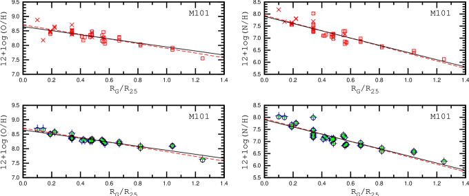
Figure 5: The radial distribution of the oxygen (left column panels) and nitrogen (right column panels) in the disc of the spiral galaxy M 101. In the upper two panels, $T_{e}$-based abundances are shown by the (red) squares (with measured $t_{3,O}$) and the (red) crosses (with measured $t_{2,N}$). The linear best fit to these data points is shown by the long-dashed (red) line. In the lower two panels, the $C$-based abundances obtained with $Rsample08$, $Rsample10$, and $Rsample12$ are shown by the (green) dots, open circles [the best fit to those data is given by the solid (black) line], and plus signs, respectively.

2.5 Verification of the $C$ method

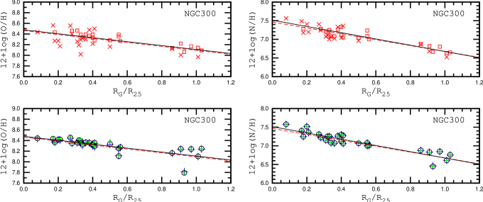
Figure 6: Same as Fig. 5 but for the disc of the spiral galaxy NGC 300.

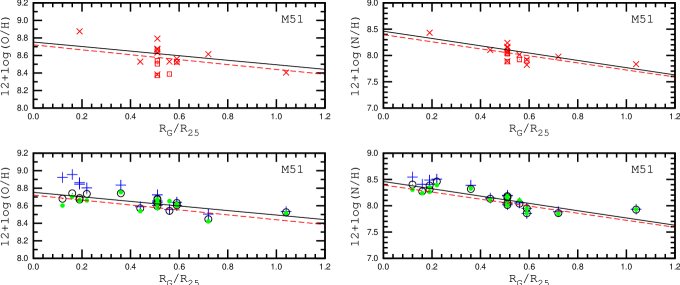
Figure 7: Same as Fig. 5 but for the disc of the spiral galaxy M 51. The (red) squares are the $T_{e}$-based abundances with measured electron temperature $t_{3,S}$. The other notations are the same as in Fig. 5.

The radial oxygen abundance distributions in the discs of the spiral galaxies M 101, NGC 300, and M 51 were derived based on H ii regions with measured electron temperatures (Kennicutt et al., 2003; Bresolin et al., 2009b, 2004), which offers a possibility to verify the $C$ method and different samples of reference H ii regions by comparing the radial distribution of the $C$-based abundances with those traced by the H ii regions with $T_{e}$-based abundances. The fractional radius, the galactocentric distance $R_{G}$ expressed in terms of the isophotal radius $R_{25}$, is used in the diagrams where radial oxygen (nitrogen) abundance distributions are plotted.

In Fig. 5 we compare the radial distributions of the oxygen and nitrogen abundances obtained by the $C$ method using different samples of reference H ii regions with radial distributions traced by $T_{e}$-based abundances in the disc of the M 101 (from the compilation by Pilyugin & Mattsson, 2011). The upper panels in Fig. 5 show the $T_{e}$-based oxygen (upper left panel) and nitrogen (upper right panel) abundances: the open (red) squares are H ii regions with measured $t_{3,O}$ electron temperatures (detected [O iii]$\lambda$4363 line) and the (red) crosses are those with measured $t_{2,N}$ electron temperatures (detected [N ii]$\lambda$5755). If both auroral lines are available then we derive two values of oxygen (or nitrogen) abundances. The long-dashed (red) line is the best linear fit to these data. The symbols in the lower panels in Fig. 5 show the $C$-method based oxygen (lower left panel) and nitrogen (lower right panel) abundances from the same sample of H ii regions. The (green) points, (blue) plus signs, and (black) open circles show abundances obtained with the $Rsample08$, $Rsample10$, and $Rsample12$ reference samples, respectively.

Fig. 5 shows that the oxygen and nitrogen abundances determined by the $C$ method using the three different reference samples are in agreement with each other and the radial distributions of the $C$-method-based oxygen and nitrogen abundances follow to the same trends traced by $T_{e}$-based abundances. Fig. 6 shows the same for the radial abundance distributions in the disc of the spiral galaxy NGC 300. The abundances of H ii regions were determined with the spectral measurements from Bresolin et al. (2009b). Again, the oxygen and nitrogen abundances derived by the $C$ method using the three different reference samples are in agreement with each other, and the radial distributions of $C$-method-based oxygen and nitrogen abundances follow almost exactly the trends traced by $T_{e}$-based abundances (the best linear fits to $T_{e}$-based and $C$-method-based abundances coincide and cannot be distinguished in Fig. 6). It should be noted that the scatter in the $C$-method-based abundances, at a given galactocentric distance, is even smaller than the one in the $T_{e}$-based abundances.

Fig. 7 compares the radial distributions of $T_{e}$-based and $C$-method-based oxygen and nitrogen abundances in the disc of the spiral galaxy M 51. The $t_{2,N}$ and $t_{3,S}$ electron temperatures have been measured in a number of H ii regions in the disc of M 51 (Bresolin et al., 2004; Garnett et al., 2004). The oxygen abundance gradient derived by Bresolin et al. (2004) is shown by the long-dashed (red) line in the upper left panel. $C$-method-based abundances for the Bresolin et al. (2004) total sample are derived including H ii regions where auroral lines were not detected (their Table 6). Fig. 7 confirms again that the oxygen and nitrogen abundances determined by the $C$ method using the three different reference samples are in agreement with each other and the radial distributions of $C$-method-based oxygen and nitrogen abundances follow to the trends traced by $T_{e}$-based abundances.

From the above, we draw two conclusions:
1. The oxygen and nitrogen abundances estimated by the $C$ method using the three different reference samples ($Rsample12$, $Rsample10$, and $Rsample08$) are in good agreement, i.e., the $C$-method-based abundances are robust.
2. The $C$-method-based oxygen and nitrogen abundances are also in agreement with the $T_{e}$-based abundances, i.e., the $C$ method produces reliable oxygen and nitrogen abundances.

2.6 Uncertainty in the $C$-based abundances, caused by errors in line intensities

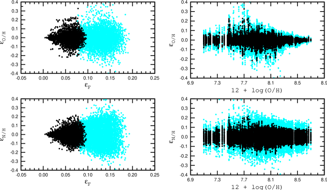
Figure 8: The error in the oxygen $\epsilon$_O/H (upper-row panels) and nitrogen $\epsilon$_N/H (lower-row panels) abundances as a function of the error in the line fluxes $\epsilon_{F}$.(left-column panels) and oxygen abundance (right-column panels). The filled dark (black) circles show the Monte Carlo simulations with random relative error in each line intensity ranging from $-10$% to $+10$%. The filled grey (light-blue in the color version) circles show these with random relative error ranging from $-20$% to $+20$%. (A color version of this figure is available in the online version.)

The “strong” nebular lines $R_{3}$ and $R_{2}$ become rather weak in high-metallicity H ii regions while the “strong” lines $N_{2}$ and $S_{2}$ are weak in low-metallicity H ii regions. Therefore the measurements of those lines can have significant errors. The uncertainty in oxygen and nitrogen abundances, caused by the uncertainty in the line flux measurements, can be estimated in the following way. We consider the measured fluxes in the reference H ii regions as the “true” fluxes and $C$-method-based oxygen and nitrogen abundances as the “true” abundances. We then introduce a random relative error $\epsilon$ to each and every line flux,

$$\begin{array}[]{lll}R_{3}^{*}&=&(1+\epsilon_{R_{3}})\;R_{3}^{\rm true},\\ &&\\ R_{2}^{*}&=&(1+\epsilon_{R_{2}})\;R_{2}^{\rm true},\\ &&\\ N_{2}^{*}&=&(1+\epsilon_{N_{2}})\;N_{2}^{\rm true},\\ &&\\ S_{2}^{*}&=&(1+\epsilon_{S_{2}})\;S_{2}^{\rm true},\\ \end{array}$$ (24)

where $\epsilon_{R_{3}}$, $\epsilon_{R_{2}}$, $\epsilon_{N_{2}}$, and $\epsilon_{S_{2}}$ are produced by a random number generator. We then determine the oxygen (O/H)${}_{C}^{*}$ and nitrogen (N/H)${}_{C}^{*}$ abundances based on the $R_{3}^{*}$, $R_{2}^{*}$, $N_{2}^{*}$, and $S_{2}^{*}$ line fluxes using the $C$ method. The differences log(O/H)${}_{C}^{*}-\log$(O/H)^true and log(N/H)${}_{C}^{*}-\log$(N/H)^true can be seen as a measure of the uncertainty in the oxygen and nitrogen abundances caused by the uncertainty in the line flux measurements.

We have considered two cases. In the first, we adopt random relative errors $\epsilon_{R_{3}}$, $\epsilon_{R_{2}}$, $\epsilon_{N_{2}}$, and $\epsilon_{S_{2}}$ in the range of $-10$% to $+10$%. The mean error in the flux measurements is defined as

$$\epsilon_{F}=\sqrt{\frac{1}{4}(\epsilon_{R_{3}}^{2}+\epsilon_{R_{2}}^{2}+\epsilon_{N_{2}}^{2}+\epsilon_{S_{2}}^{2})}.$$ (25)

The (O/H)${}_{C}^{*}$ and (N/H)${}_{C}^{*}$ abundances for each reference H ii region were computed with 50 different random errors added to each line flux. The values of the error in the oxygen and nitrogen abundances are defined as $\epsilon$_O/H = log(O/H)${}_{C}^{*}$ – log(O/H)^true and $\epsilon$_N/H = log(N/H)${}_{C}^{*}$ – log(N/H)^true, respectively. In the second case, we adopt random relative errors $\epsilon_{R_{3}}$, $\epsilon_{R_{2}}$, $\epsilon_{N_{2}}$ and $\epsilon_{S_{2}}$ in the range $-20$% to $+20$%.

The left panels in Fig. 8 show the errors in the oxygen $\epsilon$_O/H (upper panel) and nitrogen $\epsilon$_N/H (lower panel) abundances as a function of the mean error in the line fluxes $\epsilon_{F}$. The Monte Carlo simulations for the first case are shown by the dark (black) points, and those for the second case are represented by the grey (light-blue) points. In the right panels in Fig. 8 we plot the error in the oxygen $\epsilon$_O/H (upper panel) and nitrogen $\epsilon$_N/H (lower panel) abundances against the oxygen abundance.

Fig. 8 reveals that the uncertainties in the oxygen abundances caused by the errors in the first case are not in excess of 0.1 dex for the vast majority of H ii regions, although in a few cases they may be larger. The uncertainties in the nitrogen abundances are slightly larger, up to 0.15 dex. It is interesting to note that even when the mean error in the line fluxes $\epsilon_{F}$ is relatively large the error in the oxygen $\epsilon$_O/H and nitrogen $\epsilon$_N/H abundances can be close to zero. This is because the errors in the abundances caused by errors in different line intensities can have opposite signs and therefore cancel, i.e., even when the error in each term on the right-hand side of Eq. (16) is considerable, the sum (abundance) can be correct if the errors in different right-hand side terms have opposite signs and compensate each other.

A closer look at the upper right panel in Fig. 8 shows that the uncertainty in the oxygen abundance caused by errors in the line intensities reach a maximum in H ii regions with metallicities in the range from $12+\log$(O/H) $\sim 7.8$ to $12+\log$(O/H) $\sim 8.2$. This is because the strong line fluxes are less sensitive to the oxygen abundance of the H ii regions this metallicity interval (in particular, the transition from the upper to the lower branch of the R₂₃ vs. O/H diagram occurs in this interval). At high metallicities ($12+\log$(O/H) $\ga 8.2$) the uncertainty decreases with increasing metallicity. This is due to the fact that the strong line fluxes change much more with the oxygen abundance in high-metallicity (cold) H ii regions than in low-metallicity (warm and hot) H ii regions (Pilyugin et al., 2010). In other words, similar relative changes in the strong line fluxes correspond to a smaller change in the oxygen abundance in high-metallicity H ii regions than in low-metallicity H ii regions. Hence, similar relative errors in the line fluxes result in smaller errors at high metallicity than at low metallicity.

3 Application of the $C$ method: Abundance gradients in the extended discs of spiral galaxies

Spectra of H ii regions in the outer disc of the spiral galaxy M 83 (=NGC 5236) (Bresolin et al., 2009a) and in the extended disc of the spiral galaxy NGC 4625 (Goddard et al., 2011) were obtained quite recently. The abundance gradients were determined out to around 2.5 times the optical isophotal radius. It was found that at the transition between the inner and outer disc the abundance gradient becomes flatter. In addition, there appears to be an abundance discontinuity close to this transition. However, the abundances estimated with different calibrations differ by more than a factor of three. This prevents one from drawing a solid conclusion on the real behavior of the abundance gradients in the outer discs of these galaxies.

Oxygen abundance gradients have been obtained for a large sample of spiral galaxies (Vila-Costas & Edmunds, 1992; Zaritsky, 1992; van Zee et al., 1998, among others). It was found that nearly all the gradients are reasonably well fitted by a single exponential profile, although in several cases the gradient slope may not be constant across the disc but instead flattens (or steepens) in the outer disc. In particular, a break in the abundance gradient of M 101 at $R_{G}$/$R_{25}$ $\sim$ 0.5 was reported quite early on (Vila-Costas & Edmunds, 1992; Zaritsky, 1992). Oxygen abundances obtained with the strong-line method were used in those works. However, the $T_{e}$-based oxygen abundance distribution does not show the flattening in the outer disc of M 101, (upper left panel in Fig.5). It was noted in the introduction that the strong-line relations may not work across the whole range of observed metallicities in H ii regions. An unjustified use of the relationship between oxygen abundance and strong line intensities, constructed for high-metallicity H ii regions of the upper branch of the R₂₃ – O/H diagram, when determining oxygen abundances in low-metallicity H ii regions at the periphery of a galaxy, results in erroneous (overestimated) oxygen abundances, and, as a consequence, an erroneous bend in the slope of the abundance gradient (Pilyugin, 2003a).

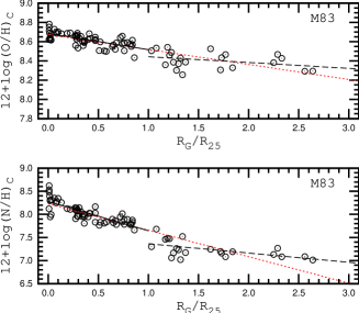
Figure 9: The radial distributions of oxygen (upper panel) and nitrogen (lower panel) abundances in the extended disc of the spiral galaxy M 83. The abundances are estimated through the $C$ method. The open circles stand for H ii regions from Dufour et al. (1980); Webster & Smith (1983); Bresolin & Kennicutt (2002); Bresolin et al. (2005, 2009a); Esteban et al. (2009). The solid line is the best linear fit to the data points with galactocentric distances smaller the isophotal $R_{25}$ radius, the dashed line is the best linear fit to data points marking the H ii regions beyond the isophotal radius. The dotted (red) line shows the best single linear fit to all the data points. (A color version of this figure is available in the online version.)

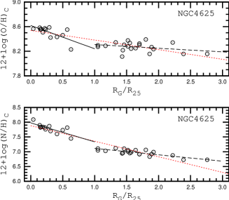
Figure 10: Same as Fig. 9 but for the spiral galaxy NGC 4625. The circles stand for the abundances in H ii regions from Goddard et al. (2011) estimated through the $C$ method. (A color version of this figure is available in the online version.)

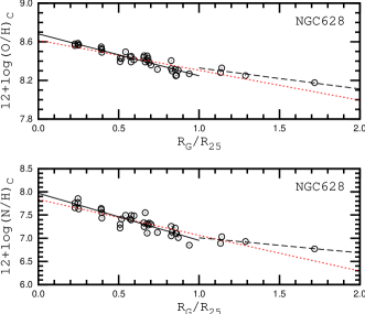
Figure 11: Same as Fig. 9 but for the spiral galaxy NGC 628. The circles represent abundances in H ii regions from McCall et al. (1985); Ferguson et al. (1998); van Zee et al. (1998); Bresolin et al. (1999) estimated through the $C$ method. (A color version of this figure is available in the online version.)

The $C$-method-based oxygen abundance distributions follow well the gradients traced by the $T_{e}$-based oxygen abundances, see Figs. 5 – 7. Here we apply the $C$ method to derive abundance gradients in the extended discs of the galaxies M 83, NGC 4652 and NGC 628. In previous works, no attention was paid to the radial distribution of nitrogen abundances in the extended discs of those galaxies, despite the fact that such studies would have several advantages (Thuan et al., 2010). First, since at $12+\log$(O/H) $\ga 8.3$, secondary nitrogen becomes dominant and the nitrogen abundance increases at a faster rate than the oxygen abundance (Henry et al., 2000), the change in nitrogen abundances with galactocentric distance should show a larger amplitude in comparison to oxygen abundances and, as a consequence, the change of the gradient and/or abundance discontinuity should be easier to detect. Furthermore, there is a time delay in the nitrogen production as compared to oxygen production (Maeder, 1992; van den Hoek & Groenewegen, 1997; Pagel, 1997; Pilyugin & Thuan, 2011). This provides an additional constraint on the chemical evolution of galaxies. These reasons led us to consider here not only the radial distribution of oxygen abundances but also that of nitrogen abundances.

Fig. 9 shows the radial distributions of the $C$-method-based oxygen and nitrogen abundances in the disc of the spiral galaxy M 83, where line measurements were taken from Dufour et al. (1980); Webster & Smith (1983); Bresolin & Kennicutt (2002); Bresolin et al. (2005, 2009a); Esteban et al. (2009). The solid line is the best linear fit to the data points with galactocentric distances smaller than the isophotal $R_{25}$ radius, and the dashed line is for the H ii regions beyond the isophotal radius. The dotted (red) line shows the best single linear fit to all the data points. Fig. 10 shows the radial distributions of oxygen and nitrogen abundances in the disc of the spiral galaxy NGC 4625 for a sample of H ii regions from Goddard et al. (2011). Fig. 11 shows the radial distributions of the oxygen and nitrogen abundances in the disc of the spiral galaxy NGC 628 for H ii regions from McCall et al. (1985); Ferguson et al. (1998); van Zee et al. (1998); Bresolin et al. (1999).

Figs. 9, 10, and 11 demonstrate that the gradient slopes within and beyond the optical isophotal radius are different. The gradient in the outer extended disc is shallower than that in the inner part of the galaxies. Thus, we confirm the conclusion of Bresolin et al. (2009a) and Goddard et al. (2011) that at the transition between the inner and outer disc the abundance gradient becomes flatter. It should be noted that the change in the gradient slope is more distinct in the radial distribution of nitrogen than oxygen abundances. This is not surprising since the change in nitrogen abundances with galactocentric distance shows a larger amplitude in comparison to oxygen abundances and, as a consequence, the change of the gradient slope is easier to detect.

On the other hand, Figs. 9, 10, and 11 do not provide a solid case in favour of the existence of an abundance discontinuity in the transition from the inner to outer disc, as was suggested by Bresolin et al. (2009a) and Goddard et al. (2011). Even if this abundance discontinuity exists, its amplitude is not in excess of the scatter in abundances among H ii regions with similar galactocentric distances.

4 Summary and conclusions

In this paper, a new way of determining abundances and electron temperatures in H ii regions based on strong emission lines is suggested. Our approach is based on the standard assumption that H ii regions with similar strong-line intensities have similar physical properties and abundances. A sample of reference H ii regions with well-measured abundances is obtained, from which we choose a counterpart for the considered H ii region by comparison of combinations of strong-line intensities. The oxygen and nitrogen abundances, as well as the electron temperature in the studied H ii region may then be assumed to be the same as that in its counterpart. In other words, we suggest a method where abundances in H ii regions are obtained “by precedent”.

To get more reliable abundances, we select a number of reference H ii regions with abundances near those in the counterpart H ii region and then derive the abundance in the studied H ii region through extra-/interpolation. We call this the counterpart method or, for brevity, the $C$ method.

We have carried out an extensive search of the literature to compile a list of individual spectra of H ii regions in irregular and spiral galaxies, with the requirement that they include the [O ii]$\lambda$3727+$\lambda$3729, [O iii]$\lambda$5007, [N ii]$\lambda$6584, [S ii]$\lambda$6717+$\lambda$6731 lines and a detected auroral line of, at least, one ion. The spectroscopic data so assembled form the basis of the present study. Our list contains 714 spectra. Since two or three auroral lines are detected in some spectra the total number of the electron temperature measurements is equal to 899. To ensure that we have a relatively homogeneous data set, we recalculated electron temperatures and oxygen and nitrogen abundances for all the H ii regions. Then we selected a sample of the reference H ii regions from the collected data. The list of our reference H ii regions ($Rsample10$) contains 414 objects.

To verify the $C$ method we considered the radial distributions of the oxygen and nitrogen abundances in the discs of the spiral galaxies M 101, NGC 300, and M 51 for which abundance gradients were established on the basis of observed H ii regions with measured electron temperatures. We found that the radial abundance gradients in the discs of these galaxies, as obtained by the $C$ method and the $T_{e}$ method, are in satisfactory agreement. This is evidence in favour of the $C$ method producing reliable abundances. Thus, the strong lines [O ii]$\lambda$3727+$\lambda$3729, [O iii]$\lambda$5007, [N ii]$\lambda$6584, and [S ii]$\lambda$6717+$\lambda$6731 allow us to estimate the oxygen and nitrogen abundances in H ii regions using the $C$ method and the resultant abundances are compatible with the $T_{e}$-based abundances. If the errors in the line measurements are within 10% then one can expect that the uncertainty in the $C$-based abundances are not in excess of 0.1 dex.

Finally, the $C$ method has been applied to study the radial abundance distributions in the extended discs of the spiral galaxies M 83, NGC 4625, and NGC 628, which have been suggested to show shallower oxygen abundance gradients in the outer disc (beyond the isophotal radius) than in the inner disc, and to investigate a discontinuity in the gradient that occurs in proximity of the optical edge of the galaxy. We confirm the conclusion of Bresolin et al. (2009a) and Goddard et al. (2011) that the abundance gradient becomes flatter at the transition between the inner and outer disc. We found that the change in the gradient slope is more distinct in the radial distribution of nitrogen than of oxygen abundances, which is expected. On the other hand, we do not find solid evidence for the existence of an abundance discontinuity at the transition from the inner to the outer disc as found by Bresolin et al. (2009a) and Goddard et al. (2011). Even if this abundance discontinuity is real its amplitude is not in excess of the scatter in abundances among H ii regions with similar galactocentric distances.

Appendix A Online material. Table A1.

Table 1 contains the dereddened line intensities, oxygen and nitrogen abundances and the electron temperatures of the reference H ii regions.

Table 1: List of the reference H ii regions. The order number of each object is shown in column 1. The dereddened line intensities (in units of H$\beta$ line flux) are given in columns 2 to 5. The $T_{e}$–based oxygen and nitrogen abundances (in units of $12+\log$(X/H)) are listed in columns 6 and 7. The electron temperature (in units of 10⁴ K) is reported in column 8. The index $j_{T}$ in column 9 is equal to 1 when the electron temperature is derived from the auroral and nebular lines of [O iii], equal to 2 when the temperature is derived from the lines of [N ii], and equal to 3 when the temperature is derived from the lines of [S iii]. (The electron temperature reduced to $t_{3}$([O iii]) is reported in all cases.) The H ii region identifier and the literature sources of the spectral data are listed in columns 10 and 11.

n	logR3	logR2	logN2	logS2	12+log(O/H)	12+log(N/H)	t3	jT	H ii region	reference
1	-0.793	0.100	0.173	-0.337	8.56	7.92	0.55	2	M51 CCM 10	Bresolin et al. (2004)
2	-0.354	0.111	0.203	-0.387	8.66	8.05	0.56	3	M51 CCM 53	Bresolin et al. (2004)
3	-0.258	0.061	0.210	-0.201	8.53	8.02	0.60	2	M51 CCM 54	Bresolin et al. (2004)
4	-0.597	-0.108	0.192	-0.387	8.63	8.16	0.50	2	M51 CCM 55	Bresolin et al. (2004)
5	-1.057	-0.201	0.124	-0.337	8.67	8.14	0.44	2	M51 CCM 72	Bresolin et al. (2004)
6	0.053	0.097	0.282	-0.469	8.53	8.10	0.66	2	M51 CCM 84A	Bresolin et al. (2004)
7	0.727	0.316	-0.534	-0.638	8.23	7.03	1.08	3	NGC1232 no 04	Bresolin et al. (2005)
8	-0.177	0.324	0.078	-0.125	8.47	7.65	0.70	2	NGC1232 no 06	Bresolin et al. (2005)
9	-0.534	0.212	0.203	-0.208	8.55	7.88	0.60	3	NGC1232 no 07	Bresolin et al. (2005)
10	0.027	0.484	0.092	-0.108	8.44	7.55	0.80	3	NGC1232 no 14	Bresolin et al. (2005)
11	-0.478	0.228	0.128	-0.180	8.61	7.84	0.59	3	NGC1365 no 05	Bresolin et al. (2005)
12	-0.285	0.320	0.083	-0.215	8.58	7.72	0.65	3	NGC1365 no 14	Bresolin et al. (2005)
13	-0.007	0.344	0.231	-0.252	8.55	7.86	0.70	2	NGC1365 no 15	Bresolin et al. (2005)
14	0.092	0.387	-0.050	-0.367	8.41	7.46	0.79	3	NGC1365 no 16	Bresolin et al. (2005)
15	0.032	0.332	0.048	-0.444	8.52	7.67	0.71	3	NGC2997 no 06	Bresolin et al. (2005)
16	-0.233	0.307	0.111	-0.252	8.53	7.73	0.67	2	NGC2997 no 07	Bresolin et al. (2005)
17	0.196	0.318	0.115	-0.367	8.56	7.80	0.72	2	NGC5236 no 03	Bresolin et al. (2005)
18	-0.922	-0.367	0.333	-0.229	8.76	8.57	0.41	2	NGC5236 no 11	Bresolin et al. (2005)
19	-0.514	0.158	0.254	-0.292	8.67	8.05	0.55	2	NGC5236 no 16	Bresolin et al. (2005)
20	0.132	0.344	-0.025	-0.526	8.47	7.57	0.75	2	M101 H 1013	Bresolin (2007)
21	0.407	0.405	-0.105	-0.523	8.44	7.46	0.85	1	M83 no 29	Bresolin et al. (2009a)
22	0.826	0.220	-0.990	-0.759	8.13	6.62	1.21	3	NGC 300 no 2	Bresolin et al. (2009b)
23	0.527	0.456	-0.567	-0.479	8.17	6.80	1.09	1	NGC 300 no 4	Bresolin et al. (2009b)
24	0.515	0.439	-0.442	-0.413	8.25	6.99	1.01	3	NGC 300 no 6	Bresolin et al. (2009b)
25	0.282	0.487	-0.343	-0.355	8.28	7.04	0.94	1	NGC 300 no 8	Bresolin et al. (2009b)
26	0.495	0.236	-0.364	-0.480	8.39	7.33	0.86	1	NGC 300 no 9	Bresolin et al. (2009b)
27	0.497	0.255	-0.593	-0.788	8.39	7.08	0.86	1	NGC 300 no 10	Bresolin et al. (2009b)
28	0.427	0.412	-0.409	-0.379	8.28	7.05	0.95	1	NGC 300 no 11	Bresolin et al. (2009b)
29	-0.399	0.418	-0.143	-0.140	8.46	7.35	0.72	3	NGC 300 no 12	Bresolin et al. (2009b)
30	0.199	0.391	-0.272	-0.426	8.32	7.20	0.86	3	NGC 300 no 13	Bresolin et al. (2009b)
31	0.382	0.394	-0.262	-0.381	8.37	7.26	0.88	1	NGC 300 no 14	Bresolin et al. (2009b)
32	0.088	0.267	-0.112	-0.319	8.36	7.46	0.78	3	NGC 300 no 15	Bresolin et al. (2009b)
33	0.102	0.422	-0.143	-0.276	8.44	7.37	0.79	3	NGC 300 no 16	Bresolin et al. (2009b)
34	0.407	0.328	-0.435	-0.564	8.39	7.16	0.85	3	NGC 300 no 17	Bresolin et al. (2009b)
35	0.196	0.413	-0.206	-0.243	8.34	7.26	0.86	3	NGC 300 no 18	Bresolin et al. (2009b)
36	0.341	0.283	-0.509	-0.514	8.32	7.07	0.86	2	NGC 300 no 19	Bresolin et al. (2009b)
37	0.480	0.164	-0.498	-0.699	8.43	7.28	0.82	1	NGC 300 no 20	Bresolin et al. (2009b)
38	0.137	0.336	-0.015	-0.256	8.44	7.56	0.77	2	NGC 300 no 21	Bresolin et al. (2009b)
39	0.010	0.431	-0.087	-0.145	8.49	7.44	0.75	3	NGC 300 no 22	Bresolin et al. (2009b)
40	0.421	0.246	-0.432	-0.553	8.40	7.24	0.83	2	NGC 300 no 23	Bresolin et al. (2009b)
41	0.379	0.294	-0.366	-0.519	8.39	7.25	0.84	1	NGC 300 no 24	Bresolin et al. (2009b)
42	0.248	0.458	-0.233	-0.347	8.47	7.29	0.81	3	NGC 300 no 25	Bresolin et al. (2009b)
43	0.537	0.204	-0.569	-0.656	8.33	7.12	0.90	1	NGC 300 no 26	Bresolin et al. (2009b)
44	0.374	0.553	-0.374	-0.088	8.14	6.88	1.11	1	NGC 300 no 27	Bresolin et al. (2009b)
45	0.511	0.497	-0.548	-0.429	8.22	6.82	1.06	1	NGC 300 no 28	Bresolin et al. (2009b)
46	0.771	0.171	-0.808	-0.726	8.18	6.87	1.11	1	Tol 1004-296 NW	Campbell et al. (1986)
47	0.714	0.347	-0.715	-0.539	8.12	6.75	1.17	1	Tol 1004-296 SE	Campbell et al. (1986)
48	0.869	0.163	-1.105	-0.699	7.95	6.46	1.43	1	Mi 462	Campbell et al. (1986)
49	0.902	0.240	-0.801	-0.613	8.13	6.82	1.26	1	Tol 0633-415	Campbell et al. (1986)
50	0.861	0.036	-1.063	-0.726	7.88	6.58	1.47	1	F 30	Campbell et al. (1986)
51	0.859	0.179	-0.912	-0.668	8.15	6.76	1.20	1	Tol 1324-276	Campbell et al. (1986)
52	0.909	0.008	-0.937	-0.646	7.97	6.80	1.41	1	Tol 1304-386	Campbell et al. (1986)
53	0.976	-0.343	-1.136	-0.983	8.06	7.02	1.33	1	II Zw 40	Campbell et al. (1986)
54	1.005	-0.116	-1.320	-0.951	8.03	6.61	1.42	1	Mi 439	Campbell et al. (1986)
55	0.985	-0.083	-1.358	-1.051	8.06	6.54	1.37	1	Tol 1334-326	Campbell et al. (1986)
56	0.859	-0.077	-1.204	-0.870	7.82	6.50	1.53	1	C 1148-203	Campbell et al. (1986)
57	0.806	0.310	-0.786	-0.572	8.16	6.76	1.18	1	Tol 1457-262 A	Campbell et al. (1986)
58	0.840	-0.108	-1.332	-0.682	7.84	6.41	1.48	1	Mrk 36	Campbell et al. (1986)

Table 1: Continued

n	logR3	logR2	logN2	logS2	12+log(O/H)	12+log(N/H)	t3	jT	H ii region	reference
59	1.026	0.048	-0.898	-0.793	8.15	6.95	1.32	1	Tol 1008-286	Campbell et al. (1986)
60	0.313	0.471	-0.181	-0.450	8.46	7.33	0.83	2	NGC 628 H13	Castellanos et al. (2002)
61	0.049	0.502	0.074	-0.218	8.50	7.55	0.78	2	NGC 1232 CDT3	Castellanos et al. (2002)
62	0.647	0.411	-0.562	-0.264	8.14	6.85	1.15	1	U 5005 (2-2)	de Blok & van der Hulst (1998)
63	0.604	0.013	-0.414	-0.674	8.31	7.45	0.91	2	M101 NGC5461	Esteban et al. (2009)
64	0.111	0.130	-0.105	-0.587	8.46	7.65	0.70	2	M101 H1013	Esteban et al. (2009)
65	0.576	0.155	-0.371	-0.801	8.47	7.46	0.83	1	M31 K9323	Esteban et al. (2009)
66	0.088	0.312	-0.217	-0.664	8.46	7.39	0.74	1	M33 NGC0595	Esteban et al. (2009)
67	0.448	0.060	-0.453	-0.595	8.33	7.35	0.84	2	M33 NGC0604	Esteban et al. (2009)
68	0.608	0.124	-0.460	-0.446	8.26	7.27	0.96	2	NGC1741 Zone C	Esteban et al. (2009)
69	0.881	-0.599	-1.646	-1.167	7.74	6.53	1.62	2	NGC2366 NGC2363	Esteban et al. (2009)
70	0.285	0.155	-0.285	-0.600	8.38	7.43	0.78	2	NGC2403 VS 24	Esteban et al. (2009)
71	0.303	0.028	-0.437	-0.733	8.40	7.40	0.76	2	NGC2403 VS 38	Esteban et al. (2009)
72	0.409	0.126	-0.392	-0.539	8.36	7.36	0.82	1	NGC2403 VS 44	Esteban et al. (2009)
73	0.907	-0.066	-1.233	-0.788	8.01	6.59	1.35	2	NGC4861 brightest	Esteban et al. (2009)
74	0.664	0.480	-0.616	-0.572	8.31	6.85	1.04	1	NGC 2403 no 5	Fierro et al. (1986)
75	0.764	0.260	-0.683	-0.481	8.06	6.84	1.24	1	II Zw 70	French (1980)
76	0.970	0.104	-1.077	-0.752	8.00	6.61	1.45	1	I Zw 122	French (1980)
77	0.911	-0.150	-1.575	-0.987	7.75	6.17	1.70	1	PHL 293 B	French (1980)
78	0.831	-0.613	-1.922	-1.509	7.48	6.08	2.03	1	Tol 1214-277	Fricke et al. (2001)
79	0.207	0.447	-0.288	-0.407	8.47	7.23	0.80	3	NHC 2403 VS 44	Garnett et al. (1997)
80	0.291	0.354	-0.359	-0.488	8.36	7.17	0.85	3	NHC 2403 VS 3	Garnett et al. (1997)
81	-0.575	0.210	0.161	-0.357	8.52	7.82	0.61	2	M51 CCM 10	Garnett et al. (2004)
82	0.997	-0.365	-1.345	-1.174	8.01	6.81	1.41	3	NGC 2363 A2	González-Delgado et al. (1994)
83	0.923	-0.149	-1.496	-1.013	7.79	6.28	1.65	1	NGC 2363 WR 185	González-Delgado et al. (1994)
84	0.887	-0.076	-1.414	-0.893	7.81	6.29	1.59	1	NGC 2363 D2	González-Delgado et al. (1994)
85	0.927	-0.114	-1.496	-0.979	7.90	6.32	1.50	1	NGC 2363 D3	González-Delgado et al. (1994)
86	0.923	-0.051	-1.399	-0.900	7.89	6.34	1.52	1	NGC 2363 B2	González-Delgado et al. (1994)
87	0.956	-0.222	-1.534	-1.036	7.92	6.41	1.49	1	NGC 2363 B3	González-Delgado et al. (1994)
88	0.963	-0.377	-1.621	-1.108	7.89	6.45	1.54	1	NGC 2363 B4	González-Delgado et al. (1994)
89	0.956	-0.301	-1.575	-1.076	7.92	6.44	1.49	1	NGC 2363 B5	González-Delgado et al. (1994)
90	0.928	-0.076	-1.496	-1.009	7.86	6.26	1.56	1	NGC 2363 WR 130	González-Delgado et al. (1994)
91	0.994	-0.076	-1.077	-0.917	8.10	6.85	1.33	1	II Zw 40	Guseva et al. (2000)
92	0.740	0.180	-0.736	-0.493	8.10	6.87	1.17	1	Mrk 1236	Guseva et al. (2000)
93	0.862	0.102	-1.120	-0.553	7.81	6.41	1.59	1	Mrk 178	Guseva et al. (2000)
94	0.748	-0.327	-1.797	-1.201	7.48	5.90	1.90	1	SBS 0940+544 Keck	Guseva et al. (2001)
95	0.749	-0.231	-1.672	-1.194	7.43	5.90	2.02	1	SBS 0940+544 MMT	Guseva et al. (2001)
96	0.821	-0.272	-1.514	-1.149	7.60	6.23	1.80	1	HS 1442+4250 c	Guseva et al. (2003a)
97	0.489	0.139	-1.057	-0.648	7.50	6.15	1.66	1	HS 1442+4250 e	Guseva et al. (2003a)
98	0.673	-0.023	-1.371	-0.815	7.59	6.08	1.66	1	SBS 1415+437 e1	Guseva et al. (2003b)
99	0.625	0.035	-1.253	-0.735	7.61	6.14	1.60	1	SBS 1415+437 e2	Guseva et al. (2003b)
100	0.910	-0.554	-1.672	-1.119	7.75	6.47	1.65	1	Pox 186	Guseva et al. (2004)
101	0.917	-0.004	-1.120	-0.860	8.05	6.68	1.32	1	J0014-0044 no 1	Guseva et al. (2009)
102	0.563	0.520	-0.564	-0.145	8.04	6.67	1.25	1	J0301-0059 no 1	Guseva et al. (2009)
103	0.439	0.112	-1.144	-0.670	7.57	6.11	1.51	1	G0405-3648 no 1	Guseva et al. (2009)
104	0.859	0.183	-1.186	-0.688	7.94	6.35	1.43	1	J2324-0006	Guseva et al. (2009)
105	0.651	0.469	-0.575	-0.300	8.15	6.80	1.16	3	UM 283 D	Guseva et al. (2011)
106	0.690	0.030	-1.385	-0.788	7.68	6.08	1.56	1	UM 133 H	Guseva et al. (2011)
107	0.728	-0.045	-1.399	-0.796	7.67	6.14	1.59	1	UM 133 O	Guseva et al. (2011)
108	0.842	0.024	-1.152	-0.721	7.95	6.54	1.36	1	UM 408	Guseva et al. (2011)
109	0.831	-0.211	-1.478	-0.975	7.66	6.25	1.72	1	UM 417	Guseva et al. (2011)
110	0.935	-0.413	-1.496	-1.009	7.88	6.60	1.50	1	MRK 600	Guseva et al. (2011)
111	0.226	0.286	-0.013	-0.523	8.51	7.66	0.74	1	HE 2-10 E	Guseva et al. (2011)
112	0.333	0.233	0.053	-0.470	8.58	7.84	0.72	2	MRK 1259	Guseva et al. (2011)
113	0.869	0.020	-1.204	-0.807	7.99	6.52	1.34	1	MRK 1271	Guseva et al. (2011)
114	0.938	-0.090	-1.332	-0.870	7.90	6.46	1.51	3	POX 4	Guseva et al. (2011)
115	0.833	-0.511	-1.973	-1.444	7.49	5.94	2.02	1	TOL 1214-277	Guseva et al. (2011)
116	0.773	0.172	-0.779	-0.569	8.07	6.83	1.21	2	NGC 5253 C2	Guseva et al. (2011)
117	0.827	0.244	-0.898	-0.724	8.19	6.73	1.16	3	NGC 5253 P1	Guseva et al. (2011)
118	0.814	0.181	-0.752	-0.684	8.19	6.93	1.14	2	TOL 89 no 1	Guseva et al. (2011)
119	1.091	0.066	-1.445	-0.924	8.01	6.32	1.57	1	NGC 5408 no 1	Guseva et al. (2011)
120	0.922	0.413	-0.962	-0.680	8.14	6.51	1.32	3	TOL 1457-262	Guseva et al. (2011)
121	0.764	-0.025	-1.019	-0.772	7.99	6.72	1.24	1	TOL 1924-416 no 1	Guseva et al. (2011)

Table 1: Continued

n	logR3	logR2	logN2	logS2	12+log(O/H)	12+log(N/H)	t3	jT	H ii region	reference
122	0.849	0.057	-1.136	-0.710	7.91	6.50	1.43	3	TOL 1924-416 no 2	Guseva et al. (2011)
123	0.890	-0.299	-1.621	-1.060	7.72	6.25	1.70	1	PHL 293 B	Guseva et al. (2011)
124	0.997	-0.321	-1.358	-1.036	7.93	6.70	1.52	1	TOL 0513-393	Guseva et al. (2011)
125	0.614	0.338	-0.550	-0.344	8.11	6.90	1.13	1	J154054+565138	Hägele et al. (2008)
126	0.913	-0.071	-1.243	-0.870	8.01	6.59	1.35	3	J161623+470202	Hägele et al. (2008)
127	0.836	0.246	-0.536	-0.638	8.22	7.12	1.13	3	J172906+565319	Hägele et al. (2008)
128	0.704	0.318	-0.418	-0.516	8.29	7.18	1.03	1	M101 NGC 5455	Hawley (1978)
129	0.692	0.161	-1.274	-0.745	7.64	6.05	1.68	1	WLM no 7	Hodge & Miller (1995)
130	0.759	0.017	-0.762	-0.469	8.03	6.95	1.21	1	WLM no 9	Hodge & Miller (1995)
131	0.574	0.023	-1.414	-0.951	7.53	5.93	1.66	1	0832+699	Izotov et al. (1994)
132	0.861	0.172	-1.070	-0.708	8.01	6.52	1.34	1	0946+558	Izotov et al. (1994)
133	0.802	0.129	-1.050	-0.699	7.97	6.54	1.32	1	1135+581	Izotov et al. (1994)
134	0.663	-0.169	-1.534	-1.018	7.41	5.94	1.94	1	1159+545	Izotov et al. (1994)
135	0.791	-0.190	-1.575	-1.022	7.64	6.10	1.70	1	1211+540	Izotov et al. (1994)
136	0.861	-0.053	-1.371	-0.921	7.78	6.29	1.60	1	1331+493N	Izotov et al. (1994)
137	0.845	0.146	-1.105	-0.642	7.94	6.46	1.41	1	1437+370	Izotov et al. (1994)
138	0.943	-0.213	-1.496	-1.066	7.84	6.38	1.59	1	0723+692A	Izotov et al. (1997)
139	0.758	0.198	-1.136	-0.708	7.82	6.29	1.49	1	0723+692B	Izotov et al. (1997)
140	0.768	0.464	-0.790	-0.369	8.02	6.53	1.36	1	0741+535	Izotov et al. (1997)
141	0.812	0.222	-0.995	-0.535	7.84	6.43	1.53	1	0749+568	Izotov et al. (1997)
142	1.021	0.101	-0.984	-0.775	8.15	6.81	1.33	1	0749+582	Izotov et al. (1997)
143	0.959	-0.027	-1.358	-0.939	7.98	6.43	1.44	1	0907+543	Izotov et al. (1997)
144	0.794	0.276	-1.113	-0.556	7.85	6.27	1.51	1	0917+527	Izotov et al. (1997)
145	0.803	0.252	-0.957	-0.484	7.92	6.49	1.43	1	0926+606	Izotov et al. (1997)
146	0.404	-0.389	-1.797	-1.292	7.15	5.64	1.93	1	0930+554	Izotov et al. (1997)
147	0.724	-0.244	-1.672	-1.143	7.41	5.89	2.02	1	0940+544N	Izotov et al. (1997)
148	0.825	-0.014	-1.385	-0.788	7.79	6.23	1.55	1	1030+583	Izotov et al. (1997)
149	0.898	0.028	-1.195	-0.799	7.99	6.53	1.38	1	1054+365	Izotov et al. (1997)
150	0.809	-0.230	-1.445	-0.876	7.67	6.29	1.67	1	1116+583B	Izotov et al. (1997)
151	0.662	0.125	-1.177	-0.750	7.69	6.20	1.54	1	1124+792	Izotov et al. (1997)
152	0.887	-0.059	-1.358	-0.873	7.75	6.29	1.69	1	1128+573	Izotov et al. (1997)
153	0.899	0.068	-1.296	-0.810	7.96	6.37	1.42	1	1222+614	Izotov et al. (1997)
154	0.868	-0.143	-1.414	-0.975	7.75	6.32	1.63	1	1223+487	Izotov et al. (1997)
155	0.887	0.042	-1.213	-0.780	8.00	6.50	1.36	1	1256+351	Izotov et al. (1997)
156	0.640	0.388	-0.669	-0.189	7.92	6.62	1.35	1	1319+579B	Izotov et al. (1997)
157	0.816	0.177	-0.957	-0.466	8.01	6.62	1.31	1	1441+294	Izotov et al. (1997)
158	0.795	0.341	-0.872	-0.441	8.09	6.60	1.26	1	1535+554	Izotov et al. (1997)
159	0.414	-0.542	-1.922	-1.432	7.12	5.64	1.98	1	I Zw 18 NW	Izotov & Thuan (1998a)
160	0.327	-0.228	-1.575	-1.155	7.15	5.69	1.89	1	I Zw 18 SE	Izotov & Thuan (1998a)
161	0.863	0.115	-1.332	-0.772	7.82	6.20	1.58	1	Mrk 600	Izotov & Thuan (1998b)
162	0.705	0.328	-0.736	-0.399	8.07	6.71	1.21	1	Mrk 5	Izotov & Thuan (1998b)
163	0.908	0.206	-0.917	-0.578	8.00	6.65	1.41	1	Mrk 1271	Izotov & Thuan (1998b)
164	0.808	0.112	-1.152	-0.697	7.82	6.36	1.52	1	Mrk 36	Izotov & Thuan (1998b)
165	0.690	0.518	-0.571	-0.287	8.17	6.78	1.19	1	Mrk 162	Izotov & Thuan (1998b)
166	0.904	-0.278	-1.554	-1.027	7.78	6.34	1.62	1	UM 461	Izotov & Thuan (1998b)
167	0.817	0.241	-1.013	-0.553	7.97	6.48	1.38	1	UM 462 SW	Izotov & Thuan (1998b)
168	0.695	-0.169	-1.554	-1.018	7.47	5.97	1.85	1	SBS 1159+545	Izotov & Thuan (1998b)
169	0.787	0.097	-1.285	-0.910	7.71	6.17	1.65	1	SBS 1249+493	Izotov & Thuan (1998b)
170	0.659	0.051	-1.332	-0.799	7.57	6.04	1.71	1	SBS 1415+437	Izotov & Thuan (1998b)
171	0.744	0.375	-0.721	-0.331	8.09	6.71	1.23	1	Mrk 930	Izotov & Thuan (1998b)
172	0.367	-0.299	-1.700	-1.161	7.15	5.64	1.92	1	I Zw 18 Southeast	Izotov et al. (1999)
173	0.684	-0.171	-1.621	-0.959	7.52	5.93	1.75	1	Tol 65	Izotov et al. (2001)
174	0.731	-0.348	-1.762	-1.119	7.47	5.94	1.89	1	Tol 65 no 1	Izotov et al. (2004)
175	0.639	-0.165	-1.496	-0.936	7.44	5.98	1.83	1	Tol 65 no 2	Izotov et al. (2004)
176	0.776	-0.143	-1.514	-0.947	7.58	6.08	1.78	1	HS 0122+0743	Izotov & Thuan (2004)
177	0.978	-0.103	-1.025	-0.796	8.16	6.96	1.25	1	HS 0128+2832	Izotov & Thuan (2004)
178	0.994	-0.186	-1.429	-0.879	7.86	6.45	1.64	1	HS 0134+3415	Izotov & Thuan (2004)
179	0.698	0.257	-1.263	-0.693	7.67	6.00	1.68	1	UM 133	Izotov & Thuan (2004)
180	0.588	0.366	-0.468	-0.391	8.25	7.04	1.02	1	Mrk 1063	Izotov & Thuan (2004)
181	0.940	0.069	-1.136	-0.767	7.97	6.55	1.45	1	HS 0811+4913	Izotov & Thuan (2004)
182	0.865	0.039	-1.371	-0.903	7.76	6.19	1.65	1	CGCG 007-025 no 1	Izotov & Thuan (2004)
183	0.783	0.194	-1.223	-0.719	7.73	6.15	1.66	1	CGCG 007-025 no 2	Izotov & Thuan (2004)
184	0.909	0.164	-0.868	-0.604	8.17	6.85	1.22	1	Mrk 1236	Izotov & Thuan (2004)

Table 1: Continued

n	logR3	logR2	logN2	logS2	12+log(O/H)	12+log(N/H)	t3	jT	H ii region	reference
185	0.853	0.176	-1.105	-0.724	8.06	6.51	1.29	1	Mrk 724	Izotov & Thuan (2004)
186	1.029	0.024	-1.233	-0.854	8.08	6.59	1.41	1	UM 439	Izotov & Thuan (2004)
187	0.726	0.442	-0.851	-0.487	8.09	6.52	1.25	1	Pox 36	Izotov & Thuan (2004)
188	0.905	0.035	-1.120	-0.907	8.01	6.62	1.36	2	Mrk 1315	Izotov & Thuan (2004)
189	0.628	0.494	-0.633	-0.511	8.26	6.78	1.07	1	HS 1213+3636A	Izotov & Thuan (2004)
190	0.887	0.148	-1.113	-0.783	8.04	6.53	1.33	1	HS 1214+3801	Izotov & Thuan (2004)
191	0.864	0.094	-1.037	-0.836	8.14	6.71	1.20	2	Mrk 1329	Izotov & Thuan (2004)
192	0.830	0.248	-0.823	-0.577	8.16	6.79	1.19	2	Mrk 450 no 1	Izotov & Thuan (2004)
193	0.842	0.237	-0.863	-0.513	8.11	6.72	1.25	1	Mrk 450 no 2	Izotov & Thuan (2004)
194	0.876	0.259	-1.037	-0.597	8.07	6.52	1.31	1	Mrk 67	Izotov & Thuan (2004)
195	0.805	-0.216	-1.646	-1.222	7.43	5.94	2.13	1	HS 2236+1344	Izotov & Thuan (2004)
196	0.933	0.087	-1.098	-0.742	8.04	6.61	1.37	1	M101 no 1	Izotov & Thuan (2004)
197	0.790	0.388	-0.709	-0.396	8.00	6.66	1.37	1	M101 no 2	Izotov & Thuan (2004)
198	0.708	0.360	-0.446	-0.519	8.36	7.16	0.99	1	M101 no 3	Izotov & Thuan (2004)
199	0.655	0.418	-0.450	-0.434	8.29	7.05	1.03	1	M101 no 4	Izotov & Thuan (2004)
200	0.622	-0.629	-1.922	-1.481	7.25	5.88	2.08	1	0335-052E n1+2 lr	Izotov et al. (2009)
201	0.606	-0.662	-1.876	-1.456	7.21	5.93	2.15	1	0335-052E n1+2 hr	Izotov et al. (2009)
202	0.422	-0.606	-1.876	-1.292	7.09	5.73	2.05	1	0335-052E n7 lr	Izotov et al. (2009)
203	0.413	-0.602	-1.973	-1.337	7.13	5.66	1.94	1	0335-052E n7 hr	Izotov et al. (2009)
204	0.238	-0.124	-1.345	-0.959	7.21	5.84	1.72	1	0335-052W n1 hr	Izotov et al. (2009)
205	0.858	-0.291	-1.646	-1.114	7.70	6.19	1.68	1	PHL 293B	Izotov et al. (2011)
206	0.786	0.445	-0.544	-0.305	8.18	6.89	1.20	1	UM 306	Kehrig et al. (2004)
207	0.742	0.449	-0.715	-0.445	8.04	6.62	1.31	1	Tol 0140-420	Kehrig et al. (2004)
208	0.948	0.182	-1.063	-0.870	8.16	6.64	1.26	1	UM 396	Kehrig et al. (2004)
209	0.840	0.277	-0.898	-0.423	7.99	6.58	1.38	1	UM 408	Kehrig et al. (2004)
210	0.798	0.332	-0.872	-0.407	7.99	6.55	1.36	1	Tol 0341-407	Kehrig et al. (2004)
211	0.772	0.399	-0.766	-0.373	7.99	6.58	1.38	1	Tol 0528-383 W	Kehrig et al. (2004)
212	0.769	0.653	-0.623	-0.322	8.13	6.60	1.33	1	Tol 0528-383 E	Kehrig et al. (2004)
213	0.957	-0.079	-0.962	-0.754	8.04	6.92	1.36	1	II Zw 40	Kehrig et al. (2004)
214	0.909	0.416	-0.736	-0.461	8.21	6.78	1.23	1	Tol 0633-415	Kehrig et al. (2004)
215	0.784	-0.105	-1.445	-0.735	7.67	6.17	1.66	1	Cam 0840+1044	Kehrig et al. (2004)
216	0.675	0.398	-0.766	-0.389	8.01	6.58	1.28	1	Tol 0957-278	Kehrig et al. (2004)
217	0.762	0.290	-0.691	-0.547	8.24	6.91	1.09	1	Tol 1004-296	Kehrig et al. (2004)
218	0.739	0.314	-0.661	-0.519	8.21	6.90	1.10	1	Tol 1004-296 SE	Kehrig et al. (2004)
219	0.954	0.375	-0.889	-0.529	8.16	6.64	1.31	1	CTS 1011	Kehrig et al. (2004)
220	0.847	0.381	-0.584	-0.491	8.26	6.97	1.15	1	CTS 1020	Kehrig et al. (2004)
221	0.780	0.452	-0.868	-0.387	8.09	6.50	1.29	1	CTS 1022	Kehrig et al. (2004)
222	0.916	0.199	-0.968	-0.606	7.98	6.60	1.44	1	Fairall 30	Kehrig et al. (2004)
223	0.741	0.203	-1.120	-0.573	7.85	6.31	1.44	1	Mkr 36	Kehrig et al. (2004)
224	0.879	0.253	-1.031	-0.507	7.96	6.46	1.45	1	UM 439	Kehrig et al. (2004)
225	0.943	0.144	-1.128	-0.320	8.02	6.52	1.41	1	UM 439 SE	Kehrig et al. (2004)
226	0.575	0.512	-0.275	-0.183	8.20	7.08	1.10	1	UM 448	Kehrig et al. (2004)
227	0.857	0.078	-1.136	-0.542	7.90	6.48	1.45	1	UM 455 NW	Kehrig et al. (2004)
228	0.797	0.311	-0.979	-0.499	7.91	6.41	1.46	1	UM 456	Kehrig et al. (2004)
229	0.840	0.185	-1.031	-0.614	7.92	6.49	1.44	1	UM 456 NE	Kehrig et al. (2004)
230	0.769	0.347	-0.942	-0.446	8.02	6.48	1.31	1	UM 456 Cent	Kehrig et al. (2004)
231	0.886	-0.103	-1.621	-0.914	7.72	6.06	1.72	1	UM 461	Kehrig et al. (2004)
232	0.917	-0.159	-1.534	-0.921	7.74	6.22	1.72	1	UM 461 E	Kehrig et al. (2004)
233	0.742	0.363	-0.973	-0.474	7.91	6.35	1.43	1	UM 462	Kehrig et al. (2004)
234	0.737	0.344	-1.057	-0.524	7.94	6.30	1.39	1	UM 462 NE	Kehrig et al. (2004)
235	0.863	0.428	-0.823	-0.450	8.11	6.60	1.32	1	UM 483	Kehrig et al. (2004)
236	0.441	0.366	-0.903	-0.450	7.68	6.21	1.52	1	DDO 155	Kehrig et al. (2004)
237	0.965	0.027	-1.160	-0.674	7.97	6.57	1.48	1	CTS 1033	Kehrig et al. (2004)
238	0.811	0.341	-0.917	-0.446	8.04	6.53	1.32	1	Tol 1457-262 SE	Kehrig et al. (2004)
239	0.652	0.552	-0.575	-0.199	8.12	6.71	1.23	1	Tol 1457-262 W	Kehrig et al. (2004)
240	0.636	0.567	-0.511	-0.208	8.14	6.77	1.21	1	Tol 1457-262W CeW	Kehrig et al. (2004)
241	0.644	0.551	-0.575	-0.202	8.08	6.68	1.27	1	Tol 1457-262W CeE	Kehrig et al. (2004)
242	0.866	0.181	-0.973	-0.623	7.97	6.59	1.40	1	Tol 1924-416	Kehrig et al. (2004)
243	0.850	0.178	-0.942	-0.622	7.98	6.63	1.37	1	Tol 1924-416 W	Kehrig et al. (2004)
244	0.885	0.182	-1.031	-0.633	7.97	6.54	1.42	1	Tol 1924-416 E	Kehrig et al. (2004)
245	0.903	-0.268	-1.098	-0.886	7.99	6.91	1.34	1	M33 MA 1	Kehrig et al. (2011)
246	0.767	0.332	-0.496	-0.377	8.15	7.01	1.18	1	M33 BCLMP 651	Kehrig et al. (2011)
247	0.470	0.207	-1.001	-0.614	7.66	6.24	1.45	1	DDO 154 no 2	Kennicutt & Skillman (2001)

Table 1: Continued

n	logR3	logR2	logN2	logS2	12+log(O/H)	12+log(N/H)	t3	jT	H ii region	reference
248	0.470	0.207	-1.001	-0.614	7.66	6.24	1.45	1	DDO 154 no 2	Kennicutt & Skillman (2001)
249	0.137	0.274	-0.066	-0.541	8.49	7.60	0.72	2	M101 H 1013	Kennicutt et al. (2003)
250	0.624	0.267	-0.352	-0.618	8.38	7.33	0.92	2	M101 H 1105	Kennicutt et al. (2003)
251	0.625	0.297	-0.503	-0.526	8.30	7.10	0.97	1	M101 H 1159	Kennicutt et al. (2003)
252	0.691	0.204	-0.550	-0.638	8.28	7.14	1.00	1	M101 H 1176	Kennicutt et al. (2003)
253	0.799	0.179	-0.831	-0.793	8.16	6.83	1.15	1	M101 H 1216	Kennicutt et al. (2003)
254	0.716	0.161	-0.558	-0.633	8.26	7.16	1.02	2	M101 H 128	Kennicutt et al. (2003)
255	0.626	0.326	-0.321	-0.429	8.34	7.29	0.96	1	M101 H 149	Kennicutt et al. (2003)
256	-0.514	0.250	0.106	-0.246	8.61	7.80	0.59	2	M101 H 336	Kennicutt et al. (2003)
257	0.692	0.338	-0.440	-0.506	8.28	7.13	1.03	2	M101 H 409	Kennicutt et al. (2003)
258	0.550	0.493	-0.503	-0.326	8.15	6.83	1.13	1	M101 H 70	Kennicutt et al. (2003)
259	0.933	0.025	-1.044	-0.801	8.05	6.74	1.33	1	M101 NGC5471-A	Kennicutt et al. (2003)
260	0.886	0.137	-0.947	-0.686	8.06	6.72	1.30	1	M101 NGC5471-D	Kennicutt et al. (2003)
261	0.480	0.288	-0.979	-0.682	7.55	6.13	1.68	1	M101 SDH 323	Kennicutt et al. (2003)
262	-0.575	0.267	0.115	-0.167	8.65	7.81	0.58	2	M101 Searle 5	Kinkel & Rosa (1994)
263	0.673	-0.480	-1.700	-1.337	7.33	6.02	2.05	1	HS 0822+3542	Kniazev et al. (2000)
264	0.772	0.295	-0.246	-0.319	8.21	7.34	1.12	1	NGC 5253 HII-2	Kobulnicky et al. (1997)
265	0.811	0.114	-0.863	-0.742	8.17	6.87	1.14	1	NGC 5253 UV-1	Kobulnicky et al. (1997)
266	0.766	0.427	-0.808	-0.585	8.18	6.64	1.18	1	POX 36	Kunth & Sargent (1983)
267	0.965	-0.057	-1.091	-0.889	8.01	6.75	1.41	1	POX 108	Kunth & Sargent (1983)
268	0.880	0.167	-1.084	-0.712	7.97	6.49	1.41	1	POX 139	Kunth & Sargent (1983)
269	0.769	0.290	-0.927	-0.662	8.03	6.55	1.28	1	Tol 2	Kunth & Sargent (1983)
270	0.853	0.314	-0.979	-0.812	8.11	6.54	1.27	1	Tol 35	Kunth & Sargent (1983)
271	1.013	-0.191	-1.144	-1.032	8.13	6.92	1.31	1	II Zw 40	Kunth & Sargent (1983)
272	0.744	0.240	-0.646	-0.879	8.42	7.12	0.94	1	M33 MA3	Kwitter & Aller (1981)
273	0.444	0.420	-0.426	-0.600	8.37	7.08	0.91	2	M33 NGC 604	Kwitter & Aller (1981)
274	0.874	0.030	-1.025	-0.936	8.07	6.74	1.26	1	M33 IC 132	Kwitter & Aller (1981)
275	0.719	0.320	-1.001	-0.378	7.92	6.36	1.38	1	WLM HM 9 (ap2)	Lee et al. (2005)
276	0.697	0.310	-0.957	-0.399	7.95	6.43	1.32	1	WLM HM 9 (ap3)	Lee et al. (2005)
277	0.670	0.405	-0.604	-0.281	8.03	6.74	1.27	1	VCC 0848-1	Lee et al. (2003a)
278	0.560	0.618	-0.471	-0.377	8.27	6.84	1.09	1	A1243-335 A	Lee et al. (2003b)
279	0.271	0.393	-0.881	-0.378	7.65	6.17	1.47	1	KISSB 23	Lee et al. (2004)
280	0.683	0.417	-0.952	-0.503	7.95	6.34	1.36	1	KISSR 73	Lee et al. (2004)
281	0.854	0.160	-1.084	-0.967	8.21	6.64	1.14	1	NGC 6822 V	Lequeux et al. (1979)
282	0.854	0.160	-0.815	-0.812	8.29	6.97	1.07	1	IC 10 no 2	Lequeux et al. (1979)
283	0.744	0.490	-0.756	-0.456	8.08	6.57	1.29	1	II Zw 70	Lequeux et al. (1979)
284	0.562	0.542	-0.468	-0.144	8.21	6.86	1.11	1	HGC 31 E	López-Sánchez et al. (2004)
285	0.861	0.207	-0.885	-0.539	8.10	6.73	1.26	1	HGC 31 F1	López-Sánchez et al. (2004)
286	0.740	0.323	-0.868	-0.479	8.08	6.60	1.23	1	HGC 31 F2	López-Sánchez et al. (2004)
287	0.610	0.614	-0.396	-0.093	8.21	6.89	1.16	1	HGC 31 G	López-Sánchez et al. (2004)
288	0.887	0.137	-0.411	-0.588	8.24	7.37	1.13	2	NGC5253 A	López-Sánchez et al. (2007)
289	0.900	0.130	-0.485	-0.648	8.22	7.29	1.16	2	NGC5253 B	López-Sánchez et al. (2007)
290	0.787	0.261	-0.804	-0.583	8.24	6.83	1.09	1	NGC5253 C	López-Sánchez et al. (2007)
291	0.601	0.548	-0.524	-0.187	8.19	6.79	1.14	3	NGC5253 D	López-Sánchez et al. (2007)
292	0.750	0.281	-0.709	-0.431	8.06	6.79	1.24	1	Mrk 5 A-INT-1	López-Sánchez & Esteban (2009)
293	0.757	0.328	-0.730	-0.418	8.07	6.73	1.24	1	Mrk 5 A-INT-2	López-Sánchez & Esteban (2009)
294	0.796	0.167	-0.309	-0.413	8.34	7.48	1.01	1	IRAS 08208-2816 C	López-Sánchez & Esteban (2009)
295	0.482	0.446	-0.283	-0.163	8.21	7.11	1.03	1	IRAS 08208-2816 3	López-Sánchez & Esteban (2009)
296	0.608	0.400	-0.299	-0.058	8.24	7.18	1.04	1	IRAS 08208-2816 5	López-Sánchez & Esteban (2009)
297	0.988	-0.000	-1.253	-0.860	8.05	6.57	1.39	1	Pox 4	López-Sánchez & Esteban (2009)
298	0.918	0.001	-1.128	-0.767	8.01	6.64	1.36	1	SBS 1054+365	López-Sánchez & Esteban (2009)
299	0.806	-0.109	-1.534	-0.979	7.65	6.08	1.72	1	SBS 1211+540	López-Sánchez & Esteban (2009)
300	0.698	0.328	-0.418	-0.450	8.21	7.12	1.08	1	III Zw 107 A	López-Sánchez & Esteban (2009)
301	0.591	0.486	-0.308	-0.194	8.31	7.14	1.01	1	III Zw 107 B	López-Sánchez & Esteban (2009)
302	0.872	0.350	-0.908	-0.510	8.05	6.55	1.36	1	Tol 1457-262 A	López-Sánchez & Esteban (2009)
303	0.842	0.272	-1.120	-0.510	7.87	6.29	1.54	1	Tol 1457-262 B	López-Sánchez & Esteban (2009)
304	0.782	0.431	-0.859	-0.323	8.03	6.50	1.34	1	Tol 1457-262 C	López-Sánchez & Esteban (2009)
305	0.433	0.408	0.197	-0.163	8.45	7.77	0.85	2	ESO 566-8	López-Sánchez & Esteban (2009)
306	0.619	0.415	-0.564	-0.551	8.24	6.90	1.05	1	IC 10 HL90	López-Sánchez et al. (2011)
307	0.696	0.233	-0.779	-0.824	8.30	6.90	1.00	1	IC 10 AP1	López-Sánchez et al. (2011)
308	0.585	0.348	-0.638	-0.484	8.24	6.87	1.02	1	IC 10 AP2	López-Sánchez et al. (2011)
309	0.689	0.312	-0.661	-0.640	8.21	6.89	1.07	1	IC 10 AP3	López-Sánchez et al. (2011)
310	0.660	0.199	-0.641	-0.770	8.21	7.00	1.03	1	IC 10 AP4	López-Sánchez et al. (2011)

Table 1: Continued

n	logR3	logR2	logN2	logS2	12+log(O/H)	12+log(N/H)	t3	jT	H ii region	reference
311	0.707	0.152	-0.885	-0.914	8.24	6.83	1.02	1	IC 10 Fib 90	López-Sánchez et al. (2011)
312	0.726	0.104	-0.917	-0.924	8.23	6.84	1.03	1	IC 10 Fib 92	López-Sánchez et al. (2011)
313	0.954	0.009	-1.001	-0.721	8.10	6.83	1.30	1	M101 NGC 5471	Luridiana et al. (2002)
314	0.692	-0.315	-0.636	-0.775	8.31	7.56	0.92	1	IC 10 no 120	Magrini & Goncalves (2009)
315	0.675	0.250	-0.648	-0.513	8.07	6.86	1.17	1	NGC 2403 -133,-146	McCall et al. (1985)
316	0.744	0.396	-0.962	-0.456	7.95	6.36	1.40	1	KISSR 396	Melbourne et al. (2004)
317	0.876	0.103	-1.136	-0.614	7.88	6.45	1.51	1	KISSR 675	Melbourne et al. (2004)
318	0.836	0.311	-0.937	-0.472	7.94	6.48	1.45	1	KISSR 1194	Melbourne et al. (2004)
319	0.677	0.038	-1.332	-0.730	7.57	6.05	1.72	1	KISSR 1752	Melbourne et al. (2004)
320	0.584	0.447	-0.730	-0.253	7.96	6.53	1.30	1	KISSR 1778	Melbourne et al. (2004)
321	0.847	0.385	-0.847	-0.437	8.08	6.59	1.32	1	KISSR 1845	Melbourne et al. (2004)
322	0.667	-0.593	-1.797	-1.444	7.36	6.05	1.95	1	SBS 0335-052 B	Melnick et al. (1992)
323	0.761	0.346	-0.876	-0.658	8.11	6.60	1.21	1	NGC 6822 X	Miller (1996)
324	0.909	0.036	-1.186	-0.775	8.03	6.56	1.35	1	Mrk 59 no 1	Noeske et al. (2000)
325	0.714	0.318	-0.736	-0.460	7.98	6.67	1.31	1	Mrk 59 no 2	Noeske et al. (2000)
326	0.674	0.560	-0.626	-0.455	8.18	6.69	1.19	1	NGC 1313 no 7	Pagel et al. (1980)
327	1.010	-0.268	-1.253	-1.108	8.10	6.87	1.33	1	II Zw 40 ld86	Pagel et al. (1992)
328	0.513	0.500	-0.136	-0.260	8.39	7.34	0.93	3	NGC 3310 C	Pastoriza et al. (1993)
329	0.974	-0.240	-1.514	-1.119	7.94	6.46	1.49	1	NGC 2366 NGC 2363	Peimbert et al. (1986)
330	0.517	0.360	-0.835	-0.469	7.70	6.31	1.53	1	NGC 3109 no 11	Peña et al. (2007)
331	0.660	0.212	-0.762	-0.319	7.80	6.61	1.43	1	NGC 3109 no 15	Peña et al. (2007)
332	0.503	0.615	-0.507	-0.187	8.07	6.67	1.25	1	II Zw 71 B	Pérez-Montero et al. (2009)
333	0.816	0.417	-0.835	-0.523	8.07	6.57	1.32	1	HS 1312+3508	Popescu & Hopp (2000)
334	0.814	0.270	-0.922	-0.456	7.90	6.50	1.47	1	HS 1330+3651	Popescu & Hopp (2000)
335	0.784	-0.033	-1.399	-0.812	7.71	6.17	1.61	1	A 1228+12	Pustilnik et al. (2002)
336	0.905	0.144	-1.253	-0.839	7.84	6.27	1.61	1	VV 131 (a)	Pustilnik et al. (2003a)
337	0.706	0.490	-0.528	-0.346	8.22	6.88	1.14	1	VV 531 (e)	Pustilnik et al. (2003a)
338	0.677	-0.514	-1.876	-1.357	7.43	5.95	1.83	1	HS 0822+3542	Pustilnik et al. (2003b)
339	0.397	-0.264	-1.672	-1.292	7.19	5.67	1.90	1	DDO 68 knot 1	Pustilnik et al. (2005)
340	0.722	-0.281	-1.597	-1.097	7.42	6.01	1.99	1	HS 2134+0400	Pustilnik et al. (2006)
341	0.954	0.160	-1.007	-0.839	8.16	6.72	1.26	1	M101 NGC 5457	Rayo et al. (1982)
342	0.634	0.390	-0.386	-0.708	8.48	7.26	0.89	1	M101 NGC 5461	Rayo et al. (1982)
343	0.632	0.442	-1.037	-0.368	7.88	6.18	1.42	1	ESO 245-G005 c	Saviane et al. (2008)
344	0.668	0.290	-0.509	-0.527	8.29	7.11	1.00	1	M101 NGC 5447 2	Sedwick & Aller (1981)
345	0.651	0.513	-0.505	-0.513	8.37	6.97	1.00	1	M101 NGC 5455	Sedwick & Aller (1981)
346	0.636	0.471	-0.426	-0.467	8.22	6.98	1.09	1	M101 NGC 5462 2	Sedwick & Aller (1981)
347	0.956	0.064	-1.070	-0.818	8.12	6.72	1.29	1	M101 NGC 5471	Sedwick & Aller (1981)
348	0.787	0.212	-0.819	-0.666	8.27	6.88	1.06	1	M101 Searle 12	Sedwick & Aller (1981)
349	0.967	0.121	-1.091	-0.851	8.11	6.65	1.32	1	M 101 NGC 5471 A	Skillman (1985)
350	0.717	0.477	-0.762	-0.319	7.99	6.51	1.37	1	M 101 NGC 5471 B	Skillman (1985)
351	0.787	0.310	-0.672	-0.569	8.11	6.84	1.22	1	M 101 NGC 5471 C	Skillman (1985)
352	0.898	0.207	-0.917	-0.785	8.21	6.78	1.18	1	M 101 NGC 5471 DL	Skillman (1985)
353	0.359	-0.332	-1.762	-1.155	7.24	5.66	1.73	1	I Zw 18 SE	Skillman & Kennicutt (1993)
354	0.414	-0.578	-1.973	-1.444	7.13	5.63	1.95	1	I Zw 18 NW	Skillman & Kennicutt (1993)
355	0.548	0.316	-0.885	-0.513	7.73	6.33	1.48	1	ESO 471-G06 no 2	Skillman et al. (2003)
356	0.484	0.045	-1.213	-0.921	7.43	6.03	1.71	1	ESO 473-G24 no 2	Skillman et al. (2003)
357	0.168	0.624	0.101	-0.229	8.49	7.50	0.85	2	M 81 no 81	Stanghellini et al. (2010)
358	0.111	0.574	0.027	-0.521	8.48	7.45	0.83	2	M 81 no 123	Stanghellini et al. (2010)
359	0.946	0.240	-1.136	-0.690	8.06	6.45	1.38	1	Tol 0341-407 E	Terlevich et al. (1991)
360	1.015	-0.355	-1.144	-0.983	8.19	7.12	1.23	1	II Zw 40	Terlevich et al. (1991)
361	0.890	0.320	-0.769	-0.585	8.21	6.82	1.20	1	Tol 0633-415	Terlevich et al. (1991)
362	0.833	0.359	-0.823	-0.719	8.26	6.75	1.13	1	Tol 1004-296 NW	Terlevich et al. (1991)
363	1.027	-0.015	-0.962	-0.754	8.17	6.96	1.30	1	Tol 1008-286	Terlevich et al. (1991)
364	0.932	0.115	-1.007	-0.690	8.09	6.71	1.31	1	Fairall 30	Terlevich et al. (1991)
365	0.831	0.320	-0.912	-0.951	8.36	6.76	1.04	1	Tol 1116-325	Terlevich et al. (1991)
366	1.012	-0.071	-1.296	-0.812	8.07	6.61	1.39	1	UM 439	Terlevich et al. (1991)
367	0.932	-0.342	-1.597	-1.143	7.76	6.36	1.68	1	UM 461	Terlevich et al. (1991)
368	0.877	0.212	-1.105	-0.754	7.95	6.42	1.45	1	UM 462 SW	Terlevich et al. (1991)
369	1.033	-0.105	-1.136	-0.936	8.11	6.84	1.35	1	Tol 1156-346	Terlevich et al. (1991)
370	0.954	0.119	-0.995	-0.710	8.08	6.72	1.34	1	Tol 1304-386	Terlevich et al. (1991)
371	0.960	-0.015	-1.243	-0.900	7.99	6.54	1.44	1	Tol 1400-411	Terlevich et al. (1991)
372	0.764	0.029	-1.358	-0.907	7.66	6.12	1.68	1	1249+493	Thuan et al. (1995)
373	0.598	0.372	-0.859	-0.333	7.89	6.42	1.35	1	1331+493S	Thuan et al. (1995)

Table 1: Continued

n	logR3	logR2	logN2	logS2	12+log(O/H)	12+log(N/H)	t3	jT	H ii region	reference
374	0.598	0.025	-1.358	-0.824	7.44	5.94	1.84	1	1415+437	Thuan et al. (1995)
375	0.810	0.352	-0.689	-0.284	8.00	6.72	1.38	1	1533+469	Thuan et al. (1995)
376	0.671	0.023	-1.308	-0.818	7.57	6.09	1.70	1	S 1415+437 1.5x5	Thuan et al. (1999)
377	0.689	-0.080	-1.414	-0.910	7.59	6.10	1.66	1	S 1415+437 1.5x0.6	Thuan et al. (1999)
378	0.604	0.330	-0.316	-0.648	8.39	7.31	0.92	1	M101 NGC 5461	Torres-Peimbert et al. (1989)
379	0.924	0.120	-0.927	-0.754	8.18	6.84	1.21	2	M101 NGC 5471	Torres-Peimbert et al. (1989)
380	0.748	0.274	-0.835	-0.602	8.13	6.71	1.17	2	NGC 55	Tüllmann et al. (2003)
381	0.733	0.475	-0.739	-0.432	8.13	6.63	1.22	1	UGC 191-1	van Zee et al. (1997)
382	0.628	0.505	-0.511	-0.228	8.13	6.81	1.19	1	UGC 191-2	van Zee et al. (1997)
383	0.447	0.482	-0.739	-0.165	7.92	6.44	1.30	1	UGC 5716-2	van Zee et al. (1997)
384	0.674	0.396	-0.872	-0.524	8.08	6.52	1.21	1	UGCA 357-1	van Zee et al. (1997)
385	0.720	0.276	-0.503	-0.602	8.24	7.10	1.06	1	NGC 1232 +135,+114	van Zee et al. (1998)
386	0.658	0.561	-0.456	-0.279	8.22	6.88	1.14	1	NGC 2805 -068,-079	van Zee et al. (1998)
387	0.670	0.493	-0.569	-0.350	8.26	6.85	1.09	1	NGC 2805 +116,-098	van Zee et al. (1998)
388	0.810	0.393	-0.779	-0.527	8.07	6.64	1.31	1	IC 2458 +002,-006	van Zee et al. (1998)
389	0.802	0.090	-1.120	-0.783	7.97	6.51	1.32	1	IC 2458 -033,-007	van Zee et al. (1998)
390	0.602	0.477	-0.571	-0.460	8.28	6.86	1.04	1	NGC 5457 -459,-053	van Zee et al. (1998)
391	0.283	-0.079	-1.399	-1.036	7.24	5.78	1.75	1	UGCA 292 no 1	van Zee (2000)
392	0.859	0.307	-0.889	-0.419	8.00	6.57	1.40	1	UGC 685/A +006,-011	van Zee & Haynes (2006)
393	0.858	0.313	-0.835	-0.424	8.03	6.64	1.36	1	UGC 685/B +006,-011	van Zee & Haynes (2006)
394	0.660	0.444	-1.031	-0.493	7.95	6.23	1.36	1	UGC 1104/B +002,+007	van Zee & Haynes (2006)
395	0.578	0.503	-0.898	-0.346	7.92	6.29	1.37	1	UGC 1104/B +004,-001	van Zee & Haynes (2006)
396	0.600	0.458	-0.641	-0.325	8.01	6.64	1.27	1	UGC 2023/B -008,+025	van Zee & Haynes (2006)
397	0.726	0.294	-0.786	-0.577	8.04	6.68	1.25	1	UGC 2023/C -006,+022	van Zee & Haynes (2006)
398	0.774	0.235	-0.776	-0.616	8.09	6.79	1.21	1	UGC 3647/A -006,-018	van Zee & Haynes (2006)
399	0.763	0.082	-1.186	-0.712	7.81	6.34	1.47	1	C 007-025/A -008,+007	van Zee & Haynes (2006)
400	0.728	0.094	-1.128	-0.767	7.85	6.40	1.39	1	C 007-025/A +000,-009	van Zee & Haynes (2006)
401	0.248	-0.040	-1.263	-0.987	7.33	5.93	1.59	1	UGCA 292/C +008,+012	van Zee & Haynes (2006)
402	0.575	0.288	-0.700	-0.238	7.90	6.65	1.29	1	UGC 9992/A +011,-003	van Zee & Haynes (2006)
403	0.515	0.327	-1.007	-0.523	7.80	6.24	1.38	1	UGC 12713/A -001,-003	van Zee & Haynes (2006)
404	0.447	0.308	-0.984	-0.593	7.61	6.13	1.57	1	GR8 -019-019	van Zee et al. (2006)
405	0.410	0.334	-0.903	-0.554	7.65	6.21	1.51	1	GR8 +008-011	van Zee et al. (2006)
406	0.441	0.333	-0.351	-0.547	8.42	7.27	0.85	1	M33 NGC 604	Vílchez et al. (1988)
407	0.790	0.042	-1.385	-0.697	7.77	6.16	1.54	1	VCC 1313	Vílchez et al. (2003)
408	0.630	0.533	-0.584	-0.212	8.07	6.68	1.26	1	VCC 848	Vílchez et al. (2003)
409	0.757	0.462	-0.783	-0.521	8.21	6.65	1.16	1	NGC 300 no 15	Webster & Smith (1983)
410	0.924	0.090	-0.478	-0.570	8.16	7.30	1.23	1	NGC 5253 no 3	Webster & Smith (1983)
411	0.888	0.173	-0.597	-0.650	8.16	7.10	1.21	1	NGC 5253 no 4	Webster & Smith (1983)
412	0.665	0.535	-0.514	-0.166	8.19	6.83	1.17	1	NGC 5253 no 5	Webster & Smith (1983)
413	0.732	0.312	-0.876	-0.793	8.32	6.75	1.02	1	NGC3359 no 3	Zahid & Bresolin (2011)
414	0.555	0.431	-0.575	-0.337	8.09	6.77	1.15	1	NGC3359 no 13	Zahid & Bresolin (2011)

References

- Aggarwal & Keenan (1999) Aggarwal K.M., Keenan F.P., 1999, ApJS, 123, 31
- Alloin et al. (1979) Alloin D., Collin-Souffrin S., Joly M., Vigroux L., 1979, A&A, 78, 200
- Andrievsky et al. (2002a) Andrievsky S.M., et al., 2002a, A&A, 381, 32
- Andrievsky et al. (2002b) Andrievsky S.M., Bersier D., Kovtyukh V.V., Luck R.E., Maciel W.J., Lépine J.R.D., Beletsky Y.V., 2002b, A&A, 384, 140
- Andrievsky et al. (2002c) Andrievsky S.M., Kovtyukh V.V., Luck R.E., Lépine J.R.D., Maciel W.J., Beletsky Y.V., 2002c, A&A, 392, 491
- Andrievsky et al. (2004) Andrievsky S.M., Luck R.E., Martin P., Lépine J.R.D., 2004, A&A, 413, 159
- Asplund et al. (2009) Asplund M., Grevesse N., Sauval A.J., Scott P., 2009, ARA&A, 47, 481
- Baldwin, Phillips & Terlevich (1981) Baldwin J.A., Phillips M.M., Terlevich R., 1981, PASP, 93, 5
- Bresolin et al. (1999) Bresolin F., Kennicutt R.C., Garnett D.R., 1999, ApJ, 510, 104
- Bresolin & Kennicutt (2002) Bresolin F., Kennicutt R.C., 2002, ApJ, 572, 838
- Bresolin et al. (2004) Bresolin F., Garnett D.R., Kennicutt R.C., 2004, ApJ, 615, 228
- Bresolin et al. (2005) Bresolin F., Schaerer D., González Delgado R.M., Stasińska G., 2005, A&A, 441, 981
- Bresolin (2007) Bresolin F., 2007, ApJ, 656, 186
- Bresolin et al. (2009a) Bresolin F., Ryan-Weber E., Kennicutt R.C., Goddard Q., 2009a, ApJ, 695, 580
- Bresolin et al. (2009b) Bresolin F., Gieren W., Kudritzki R.-P., Pietrzyński G., Urbaneja M.A., Carraro G., 2009b, ApJ, 700, 309
- Campbell et al. (1986) Campbell A., Terlevich R., Melnick J., 1986, MNRAS, 223, 811
- Castellanos et al. (2002) Castellanos M., Díaz A.I., Terlevich E., 2002, MNRAS, 329, 315
- Cid Fernandes et al. (2011) Cid Fernandes R., Stasińska G., Mateus A., Asari N.V., 2011, MNRAS, 413, 1687
- de Blok & van der Hulst (1998) de Blok W.J.G., van der Hulst J.M., 1998, A&A, 335, 421
- Dopita & Evans (1986) Dopita M.A., Evans I.N., 1986, ApJ, 307, 431
- Dufour et al. (1980) Dufour R.J., Talbot R.J., Jensen E.B., Shields G.A., 1980, ApJ, 236, 119
- Edlén (1985) Edlén B., 1985, Phys. Scripta, 31, 345
- Esteban et al. (2004) Esteban C., Peimbert M., García-Rojas J., Ruiz M. T., Peimbert A., Rodríguez M., 2004, MNRAS, 355, 229
- Esteban et al. (2009) Esteban C., Bresolin F., Peimbert M., García-Rojas J., Peimbert A., Mesa-Delgado A., 2009, ApJ, 700, 654
- Ferguson et al. (1998) Ferguson A.M.N., Gallagher J.S., Wyse R.F.G., 1998, AJ, 116, 673
- Fierro et al. (1986) Fierro J., Torres-Peimbert S., Peimbert M., 1986, PASP, 98, 1032
- French (1980) French H.B., 1980, ApJ, 240, 41
- Fricke et al. (2001) Fricke K.J., Izotov Y.I., Papaderos P., Guseva N.G., Thuan T.X., 2001, AJ, 121, 169
- Froese Fisher & Tachiev (2004) Froese Fischer C., Tachiev G., 2004, ADNDT, 87, 1
- Henry et al. (2000) Henry R.B.C., Edmunds M.G., Kóppen J., 2000, ApJ, 541, 660
- Galavís et al. (1997) Galavís M.E., Mendoza C., Zeippen C.J., 1997, A&AS, 123, 159
- García-Rojas et al. (2004) García-Rojas J., Esteban C., Peimbert M., Rodríguez M., Ruiz M. T., Peimbert A. 2004, ApJS, 153, 501
- García-Rojas et al. (2005) García-Rojas J., Esteban C., Peimbert A., Peimbert M., Rodríguez M., Ruiz M.T., 2005, MNRAS, 362, 301
- García-Rojas et al. (2006) García-Rojas J., Esteban C., Peimbert M., Costado M.T., Rodríguez M., Peimbert A., Ruiz M. T. 2006, MNRAS, 368, 253
- García-Rojas & Esteban (2007) García-Rojas J., Esteban C., 2007, ApJ, 670, 457
- Garnett (1992) Garnett D.R., 1992, AJ, 103, 1330
- Garnett et al. (1997) Garnett D.R., Shields G.A., Skillman E.D., Sagan S.P., Dufour R.J., 1997, ApJ, 489, 63
- Garnett et al. (2004) Garnett D.R., Kennicutt R.C., Bresolin F., 2004, ApJ, 607, L21
- Goddard et al. (2011) Goddard Q., Bresolin F., Kennicutt R.C., Ryan-Weber E.V., Rosales-Ortega F.F., 2011, MNRAS, 412, 1246
- González-Delgado et al. (1994) González-Delgado R.M., et al., 1994, ApJ, 437, 239
- Guseva et al. (2000) Guseva N.G., Izotov Y.I., Thuan T.X., 2000, ApJ, 531, 776
- Guseva et al. (2001) Guseva N.G., et al., 2001, A&A, 378, 756
- Guseva et al. (2003a) Guseva N.G., Papaderos P., Izotov Y.I., Green R.F., Fricke K.J., Thuan T.X., Noeske K.G., 2003a, A&A, 407, 91
- Guseva et al. (2003b) Guseva N.G., Papaderos P., Izotov Y.I., Green R.F., Fricke K.J., Thuan T.X., Noeske K.G., 2003b, A&A, 407, 105
- Guseva et al. (2004) Guseva N.G., Papaderos P., Izotov Y.I., Noeske K.G., Fricke K.J., 2004, A&A, 421, 519
- Guseva et al. (2009) Guseva N.G., Papaderos P., Meyer H.T., Izotov Y.I., Fricke K.J., 2009, A&A, 505, 63
- Guseva et al. (2011) Guseva N.G., Izotov Y.I., Stasińska G., Fricke K.J., Henkel C., Papaderos P., 2011, A&A, 529, A149
- Hägele et al. (2008) Hägele G.F., Díaz Á.I., Terlevich E., Terlevich R., Pérez-Montero E., Cardaci M.V., 2008, MNRAS, 383, 209
- Hawley (1978) Hawley S.A., 1978, ApJ, 224, 417
- Hodge & Miller (1995) Hodge P., Miller B.W., 1995, ApJ, 451, 176
- Hudson & Bell (2005) Hudson C.E., Bell K.L., 2005, A&A, 430, 725
- Izotov et al. (1994) Izotov Y.I., Thuan T.X., Lipovetsky V.A., 1994, ApJ, 435, 647
- Izotov et al. (1997) Izotov Y.I., Thuan T.X., Lipovetsky V.A., 1997, ApJS, 108, 1
- Izotov & Thuan (1998a) Izotov Y.I., Thuan T.X., 1998a, ApJ, 497, 227
- Izotov & Thuan (1998b) Izotov Y.I., Thuan T.X., 1998b, ApJ, 500, 188
- Izotov et al. (1999) Izotov Y.I., Chaffee F.H., Foltz C.B., Green R.F., Guseva N.G., Thuan T.X., 1999, ApJ, 527, 757
- Izotov et al. (2001) Izotov Y.I., Chaffee F.H., Green R.F., 2001, ApJ, 562, 727
- Izotov et al. (2004) Izotov Y.I., Papaderos P., Guseva N. G., Fricke K.J., Thuan T.X., 2004, A&A, 421, 539
- Izotov & Thuan (2004) Izotov Y.I., Thuan T.X., 2004, ApJ, 602, 200
- Izotov et al. (2005) Izotov Y.I., Thuan T.X., Guseva N.G., 2005, ApJ, 632, 210
- Izotov et al. (2006) Izotov Y.I., Stasińska G., Meynet G., Guseva N.G., Thuan T.X., 2006, A&A, 448, 955
- Izotov et al. (2009) Izotov Y.I., Guseva N.G., Fricke K.J., Papaderos P., 2009, A&A, 503, 61
- Izotov et al. (2011) Izotov Y.I., Guseva N.G., Fricke K.J., Henkel C., 2011, A&A, 533, A25
- Johansson et al. (1992) Johansson L., Magnusson C.E., Joelsson I., Zetterberg P.O., 1992, Phys. Scripta, 46, 221
- Kauffmann et al. (2003) Kauffmann G., et al., 2003, MNRAS, 346, 1055
- Kehrig et al. (2004) Kehrig C., Telles E., Cuisinier F., 2004, AJ, 128, 1141
- Kehrig et al. (2011) Kehrig C., et al., 2011, A&A, 526, A128
- Kennicutt & Skillman (2001) Kennicutt R.C., Skillman E.D., 2001, AJ, 121, 1461
- Kennicutt et al. (2003) Kennicutt R.C., Bresolin F., Garnett D.R., 2003, ApJ, 591, 801
- Kewley et al. (2001) Kewley L.J., Dopita M.A., Sutherland R.S., Heisler C.A., Trevena J., 2001, ApJ, 556, 121
- Kewley & Dopita (2002) Kewley L.J., Dopita M.A., 2002, ApJS, 142, 35
- Kewley & Ellison (2008) Kewley L.J., Ellison S.L., 200, ApJ, 681, 1183
- Kinkel & Rosa (1994) Kinkel U., Rosa M.R., 1994, A&A, 282, L37
- Kniazev et al. (2000) Kniazev A.Y., et al., 2000, A&A, 357, 101
- Kniazev et al. (2004) Kniazev A.Y., Pustilnik S.A., Grebel E.K., Lee H., Pramskij A.G., 2004, ApJS, 153, 429
- Kobulnicky et al. (1997) Kobulnicky H.A., Skillman E.D., Roy J.-R., Walsh J.R., Rosa M.R., 1997, ApJ, 477, 679
- Kobulnicky & Skillman (1998) Kobulnicky H.A., Skillman E.D., 1998, ApJ, 497, 601
- Kunth & Sargent (1983) Kunth D., Sargent W.L.W., 1983, ApJ, 273, 81
- Kwitter & Aller (1981) Kwitter K.B., Aller L.H., 1981, MNRAS, 195, 939
- Lee et al. (2003a) Lee H., McCall M.L., Richer M.G., 2003a, AJ, 125, 2975
- Lee et al. (2003b) Lee H., Grebel E.K., Hodge P.W., 2003b, A&A, 401, 141
- Lee et al. (2005) Lee H., Skillman E.D., Venn K.A., 2005, ApJ, 620, 223
- Lee et al. (2004) Lee J.C., Salzer J.J., Melbourne J., 2004, ApJ, 616, 752
- Lequeux et al. (1979) Lequeux J., Peimbert M., Rayo J.F., Serrano A., Torres-Peimbert S., 1979, A&A, 80, 155
- López-Sánchez et al. (2004) López-Sánchez Á.R., Esteban C., Rodríguez M., 2004, ApJS, 153, 243
- López-Sánchez et al. (2007) López-Sánchez Á.R., Esteban C., García-Rojas J., Peimbert M., Rodríguez M., 2007, ApJ, 656, 168
- López-Sánchez & Esteban (2009) López-Sánchez Á.R., Esteban C., 2008, A&A, 508, 615
- López-Sánchez & Esteban (2010) López-Sánchez Á.R., Esteban C., 2010, A&A, 517, A85
- López-Sánchez et al. (2011) López-Sánchez Á.R., Mesa-Delgado A., López-Martín L., Esteban C., 2011, MNRAS, 411, 2076
- Luridiana et al. (2002) Luridiana V., Esteban C., Peimbert M., Peimbert A., 2002, Rev. Mex. A.A, 38, 97
- Maeder (1992) Maeder A., 1992, A&A, 264, 105
- Magrini & Goncalves (2009) Magrini L., Goncalves D.R., 2009, MNRAS, 398, 280
- Mattsson (2010) Mattsson L., 2010, A&A, 515, A68
- McCall et al. (1985) McCall M.L., Rybski P.M., Shields G.A., 1985, ApJS, 57, 1
- McGaugh (1991) McGaugh S.S., 1991, ApJ, 380,, 140
- Melbourne et al. (2004) Melbourne J., Phillips A., Salzer J.J., Gronwall C., Sarajedini V.L., 2004, AJ, 127, 686
- Melnick et al. (1992) Melnick J., Heydari-Malayeri M., Leisy P., 1992, A&A, 253, 16
- Mendoza & Zeippen (1982) Mendoza C., Zeippen C.J., 1982, MNRAS, 199, 1025
- Miller (1996) Miller B.W., 1996, AJ, 112, 991
- Moustakas et al. (2010) Moustakas J., Kennicutt R.C., Tremonti C.A., Dale D.A., Smith J.-D.T., Calzetti D., 2010. ApJS, 190, 233
- Noeske et al. (2000) Noeske K.G., Guseva N.G., Fricke K.J., Izotov Y.I., Papaderos P., Thuan T.X., 2000, A&A, 361, 33
- Pagel (1997) Pagel B.E.J., 1997, Nucleosynthesis and Chemical Evolution of Galaxies (Cambridge: Cambridge Univ. Press)
- Pagel et al. (1979) Pagel B.E.J., Edmunds M.G., Blackwell D.E., Chun M.S., Smith G., 1979, MNRAS, 189, 95
- Pagel et al. (1980) Pagel B.E.J., Edmunds M.G., Smith G., 1980, MNRAS, 193, 219
- Pagel et al. (1992) Pagel B.E.J., Simonson E.A., Terlevich R.J., Edmunds M.G., 1992, MNRAS, 255, 325
- Pastoriza et al. (1993) Pastoriza M.G., Dottori H., Terlevich E., Terlevich R., Díaz A.I. 1993, MNRAS, 260, 177
- Peimbert (2003) Peimbert A. 2003, ApJ, 584, 735
- Peimbert et al. (2005) Peimbert A., Peimbert M., Ruiz M.T. 2005, ApJ, 634, 1056
- Peimbert (1967) Peimbert M., 1967, ApJ, 150, 825
- Peimbert & Costero (1969) Peimbert M., Costero R., 1969, Bol. Obs. Tonantzintla y Tacubaya, 5, 3
- Peimbert et al. (1986) Peimbert M., Pena M., Torres-Peimbert S., 1986, A&A, 158, 266
- Peña et al. (2007) Peña M., Stasińska G., Richer M.G., 2007, A&A, 476, 745
- Peña-Guerrero et al. (2012) Peña-Guerrero M.A., Peimbert A., Peimbert M., Ruiz M.T. 2012, ApJ, 746, 115
- Pérez-Montero et al. (2009) Pérez-Montero E., García-Benito R., Díaz A.I., Pérez E., Kehrig C., 2009, A&A, 497, 53
- Pettini & Pagel (2004) Pettini M., Pagel B.E.J., 2004, MNRAS, 348, 59L
- Pilyugin (2000) Pilyugin L.S., 2000, A&A, 362, 325
- Pilyugin (2001) Pilyugin L.S., 2001, A&A, 369, 594
- Pilyugin (2003a) Pilyugin L.S., 2003, A&A, 397, 109
- Pilyugin (2003b) Pilyugin L.S., 2003, A&A, 399, 1003
- Pilyugin et al. (2003) Pilyugin L.S., Thuan, T.X., Vílchez J.M., 2003, A&A, 397, 487
- Pilyugin et al. (2004) Pilyugin L.S., Vílchez J.M., Contini T., 2004, A&A, 425, 849
- Pilyugin & Thuan (2005) Pilyugin L.S., Thuan T.X., 2005, ApJ, 631, 231
- Pilyugin et al. (2006) Pilyugin L.S.,Thuan T.X., Vílchez J.M., 2006, MNRAS, 367, 1139
- Pilyugin et al. (2010) Pilyugin L.S., Vílchez J.M., Thuan T.X., 2010, ApJ, 720, 1738
- Pilyugin & Mattsson (2011) Pilyugin L.S., Mattsson L., 2011, MNRAS, 412, 1145
- Pilyugin & Thuan (2011) Pilyugin L.S., Thuan T.X., 2011, ApJ, 726, L23
- Pilyugin et al. (2012) Pilyugin L.S., Vílchez J.M., Mattsson L., Thuan T.X., 2012, MNRAS, 421, 1624
- Popescu & Hopp (2000) Popescu C.C., Hopp U., 2000, A&AS, 142, 247
- Pradhan et al. (2006) Pradhan A.K., Montenegro M., Nahar S.N., Eissner, W., 2006, MNRAS, 366, L6
- Pustilnik et al. (2002) Pustilnik S.A., Kniazev A.Y., Masegosa J., Márquez I M., Pramskij A.G., Ugryumov A.V., 2002, A&A, 389, 779
- Pustilnik et al. (2003a) Pustilnik S., Zasov A., Kniazev A., Pramskij A., Ugryumov A., Burenkov A., 2003a, A&A, 400, 841
- Pustilnik et al. (2003b) Pustilnik S.A., Kniazev A.Y., Pramskij A.G., Ugryumov A.V., Masegosa J., 2003b, A&A, 409, 917
- Pustilnik et al. (2005) Pustilnik S.A., Kniazev A.Y., Pramskij A.G., 2005, A&A, 443, 91
- Pustilnik et al. (2006) Pustilnik S.A., Engels D., Kniazev A.Y., Pramskij A.G., Ugryumov A.V., Hagen H.-J., 2006, AstL, 32, 228
- Rayo et al. (1982) Rayo J.F., Peimbert M., Torres-Peimbert S., 1982, ApJ, 255, 1
- Rodríguez & García-Rojas (2010) Rodríguez M., García-Rojas J., 2010, ApJ, 708, 1551
- Saviane et al. (2008) Saviane I., Ivanov V.D., Held E.V., Alloin D., Rich R.M., Bresolin F., Rizzi L., 2008, A&A, 487, 901
- Sedwick & Aller (1981) Sedwick K.E., Aller L.H., 1981, Proc. Nat. Acad. Sci. USA., 78, 1994
- Skillman (1985) Skillman E.D., 1985, ApJ, 290, 449
- Skillman & Kennicutt (1993) Skillman E.D., Kennicutt R.C., 1993, ApJ, 411, 655
- Skillman et al. (2003) Skillman E.D., Côté S., Miller B.W., 2003, AJ, 125, 610
- Stanghellini et al. (2010) Stanghellini L., Magrini L., Villaver E., Galli D., 2010, A&A, 521, A3
- Stasińska (2005) Stasińska G., 2005, A&A, 434, 507
- Stasińska (2006) Stasińska G., 2006, A&A, 454, L127
- Stasińska et al. (2006) Stasińska G., Cid Fernandes R., Mateus A., Sodré L., Asari N.V., 2006, MNRAS, 371, 972
- Stasińska et al. (2008) Stasińska G., Asari N.V., Cid Fernandes R., Gomes J.M., Schlickmann M., Mateus A., Schoenell W., Sodré L., 2008, MNRAS, 391, L29
- Storey & Zeippen (2000) Storey P.J., Zeippen C.J., 2000, MNRAS, 312, 813
- Tayal & Gupta (1999) Tayal S.S., Gupta G.P., 1999, ApJ, 526, 544
- Terlevich et al. (1991) Terlevich R., Melnick J., Masegosa J., Moles M., Copetti M.V.F., 1991, A&AS, 91, 285
- Thuan et al. (1995) Thuan T.X., Izotov Y.I., Lipovetsky V.A., 1995, ApJ, 445, 108
- Thuan et al. (1999) Thuan T.X., Izotov Y.I., Foltz C.B., 1999, ApJ, 525, 105
- Thuan et al. (2010) Thuan T.X., Pilyugin L.S., Zinchenko I.A., 2010, ApJ , 712, 1029
- Torres-Peimbert et al. (1989) Torres-Peimbert S., Peimbert M., Fierro J., 1989, ApJ, 345, 186
- Tremonti et al. (2004) Tremonti C.A., et al., 2004, ApJ, 613, 898
- Tsamis et al. (2003) Tsamis Y.G., Balrlow M.J., Liu X.-W., Danziger I.J., Storey, P.J., 2003, MNRAS, 338, 687
- Tüllmann et al. (2003) Tüllmann R., Rosa M.R., Elwert T., Bomans D.J., Ferguson A.M.N., Dettmar R.-J., 2003, A&A, 412, 69
- van den Hoek & Groenewegen (1997) van den Hoek L.B., Groenewegen M.A.T., 1997, A&AS, 123, 305
- van Zee et al. (1997) van Zee L., Haynes M.P., Salzer J.J., 1997, AJ, 114, 2479
- van Zee et al. (1998) van Zee L., Salzer J.J., Haynes M.P., O‘Donoghiu A.A., Balonek T.J., 1998, AJ, 116, 2805
- van Zee (2000) van Zee L., 2000, ApJ, 543, L31
- van Zee & Haynes (2006) van Zee L., Haynes M.P., 2006, ApJ, 636, 214
- van Zee et al. (2006) van Zee L., Skillman E.D., Haynes M.P., 2006, ApJ, 637, 269
- Vila-Costas & Edmunds (1992) Vila-Costas M.B., Edmunds M.G., 1992, MNRAS, 259, 121
- Vílchez et al. (1988) Vílchez J.M., Pagel B.E.J., Díaz A.I., Terlevich E., Edmunds M.G., 1988, MNRAS, 235, 633
- Vílchez et al. (2003) Vílchez J.M., Iglesias-Páramo J., 2003, ApJS, 145, 225
- Webster & Smith (1983) Webster B.L., Smith M.G., 1983, MNRAS, 204, 743
- Wenåker (1990) Wenåker I., 1990, Phys. Scripta, 42, 667
- Williams et al. (2008) Williams R., Jenkins E.B., Baldwin J.A., Zhang Y., Sharpee B., Pellegrini E., Phillips M., 2008, ApJ, 677, 1100
- Yin et al. (2007) Yin S.Y., Liang Y.C., Hammer F., Brinchmann J., Zhang B., Deng L.C., Flores H., 2007, A&A, 462, 535
- York et al. (2000) York D.G., et al., 2000, AJ, 120, 1579
- Zahid & Bresolin (2011) Zahid H.J., Bresolin F., 2011, AJ, 141, 192
- Zaritsky (1992) Zaritsky D., 1992, ApJ, 390, L73
- Zaritsky et al. (1994) Zaritsky D., Kennicutt R.C., Huchra J.P., 1994, ApJ, 420, 87