Three-body breakup within the fully discretized Faddeev equations

Abstract

A novel approach is developed to find the three-body breakup amplitudes and cross sections within the modified Faddeev equation framework. The method is based on the lattice-like discretization of the three-body continuum with a three-body stationary wave-packet basis in momentum space. The approach makes it possible to simplify drastically all the three- and few-body breakup calculations due to discrete wave-packet representations for the few-body continuum and simultaneous lattice representation for all the scattering operators entering the integral equation kernels. As a result, the few-body breakup can be treated as a particular case of multi-channel scattering in which part of the channels represents the true few-body continuum states. As an illustration for the novel approach, an accurate calculations for the three-body breakup process $n+d\to n+n+p$ with non-local and local $NN$ interactions are calculated. The results obtained reproduce nicely the benchmark calculation results using the traditional Faddeev scheme which requires much more tedious and time-consuming calculations.

I Introduction

The last decades have inaugurated great success in precise ab-initio calculations for few-body scattering processes Gloeckle_rep ; F2 ; Elster ; Fonseca ; F1 ; Sauer ; Kievsky . These calculations made it possible to describe accurately the results of numerous recent experiments on elastic $nd$ scattering at energies up to 350 MeV and also the three-body breakup $n+d\to n+n+p$ at low and moderate energies $E_{n}\simeq 10\div 30$ MeV. However some problems remain unsettled even at such low energies. These are the so-called $A_{y}$-puzzle (as well as other puzzles for various tensor and vector analyzing powers) in elastic scattering, the problems with an adequate description of the pairwise ${}^{1}S_{0}$-channel contribution to three-body breakup at low energies Gloeckle_nn and breakup cross section in some particular three-particle configurations such as the quasi-free scattering Ruan and the space-star S_star configurations. The most plausible reason for the visible discrepancies with experimental data in this area is likely not insufficient accuracy of numerical calculations but rather some deficiency in the input $2N$- and $3N$-interactions. At the same time, the progress in the field of precise few-nucleon calculations, particularly in testing of new models for $3N$-interactions, is restrained strongly by a high number of very complicated few-nucleon calculations, especially above the three-body threshold. Because of these complications of traditional computational schemes for the direct solution of the Faddeev–Yakubovsky equations, one observes a rise of interest in recent years in alternative approaches Carbonell ; LIT ; Gl_Raw to calculate the scattering observables by simpler methods.

Among such alternative approaches one can note a preference for the so called $L_{2}$-methods. These methods are based on expansions of the scattering solution into a basis of square-integrable functions levin ; Kurouglu ; mccurthy ; horse ; papp ; Piyadasa ; Rawitscher ; CDCC_br . Such $L_{2}$-methods proved to be very well suited and quite efficient for numerous applications. One of the most successful approaches of this type is the Continuum-Discretized Coupled-Channel (CDCC) method developed three decades ago for treatment of breakup processes in direct nuclear reactions Piyadasa ; Rawitscher ; CDCC_br ; Thompson . The CDCC approach in its traditional form was unable to treat other channels than elastic scattering and projectile (or target) breakup. Recently a few groups generalized the traditional CDCC approach to scattering of three-fragment projectiles by a stable target CDCC_br . However this generalized approach can be considered as a hybrid method: $L_{2}$ discretization of inner motion in the three-body projectile and the traditional treatment of a coupled-channel problem

On the other hand, the present authors have developed some alternative $L_{2}$-technique Moro ; KPR1 ; KPR2 ; K2 which is based on the idea of complete continuum discretization with a special stationary wave-packet basis in momentum space (three-body lattice basis). The basic distinction of such an approach from the traditional CDCC-scheme for the three-body systems is that the wave-packet approach is dealing with a full discretization of the three-body continuum. In other words, the discretization on both Jacobi coordinates is used here rather than the discretization on the alone coordinate of the projectile inner motion as in the CDCC approach.

Our approach with the global discretization over all valence coordinates leads immediately to a few important advantages in the accurate treatment of few-body scattering. Among those the following are the most important:

• The few-body scattering problem is consistently formulated in a Hilbert space of three-body normalized states, similarly to the bound-state problem.

• The approach employs the integral equation framework of scattering theory instead of the differential equation approach (e.g. in the CDCC) where the boundary conditions in few-body scattering channels are not easy to formulate, especially in terms of the $L_{2}$ basis used. Contrary to this, the integral equation formulation allows to avoid any explicit account of the boundary conditions.

• When working within the wave-packet formulation of the scattering problem one can derive explicit formulas for some scattering operators (e.g. channel resolvents). Such fully analytical finite-dimensional approximations, being substituted into integral equation kernels, lead immediately to their algebraic matrix analogues. Thus, our final equations are simple matrix linear equations with regular matrices.

In our previous works KPR1 ; KPR2 we have demonstrated how to find the elastic $2\to 2$ scattering amplitudes in lattice representation. In the present paper, we generalize the technique to the three-body breakup treatment. So we present here the complete formalism for determination of three-body breakup amplitudes. It is important to emphasize in this connection that the accurate treatment of three-body breakup within the $L_{2}$ type approach is much less obvious than that of elastic ones and thus requires some additional delicate theoretical studies. In particular, the matrix elements in the breakup amplitude are not truncated over all spatial coordinates (in contrast to the elastic and rearrangement amplitudes), so the validity of the $L_{2}$ scheme in the treatment of the breakup processes should be studied carefully. As some substantiation for such approach one can consider the three-body breakup calculations within the CDCC-approach where the discretization of the continuum in the projectile inner subHamiltonian has been used for the description of the breakup amplitudes CDCC_br ; Thompson . So, the natural generalization of such a partial continuum discretization to the case of full three- and few-body continuum within the Faddeev equation approach is an important next step. Moreover, this fully discretized approach studied in the present work allows to simplify drastically all calculations and makes it more universal and elegant.

The present work has the following structure. In the section II, a three-body lattice-like free wave-packet basis is described in detail together with a similar basis for the channel Hamiltonian. Here we also discuss the properties of these bases. The complete formalism for elastic scattering and breakup, as applied to the $nd$-system in the packet representation is presented in Section III. In the Section IV, a few useful numerical illustrations and their comparison with the standard Faddeev benchmark calculations are given. Our results are summarized in the Section V. For the sake of convenience for the reader we add three appendices. In Appendix A we describe the detailed scheme for calculation of the three-body overlap matrix in the three-body lattice basis for recoupling of different Jacobi coordinates. In Appendix B we give the convenient wave-packet formalism for the solution of three-body scattering problem with separable pairwise interactions. In the last Appendix C we discuss some features of our numerical calculations.

II Lattice representation for the three-body continuum

We consider here the problem of a scattering of three identical particles 1, 2 and 3 (nucleons) with mass $m$, interacting via pairwise short-range potentials $v_{a}$ $(a=1,2,3)$. It is convenient to use three Jacobi momentum sets $({\bf p}_{a},{\bf q}_{a})$ corresponding to three channel Hamiltonians $H_{a}$ $(a=1,2,3)$ which define the asymptotic states of the system. For example, the channel Hamiltonian $H_{1}$ has the form of the direct sum of two-body subHamiltonians

$$H_{1}\equiv h_{1}\oplus h_{0}^{1},$$ (1)

where subHamiltonian $h_{1}$ describes $NN$ subsystem consisting of particles 2 and 3 with interaction $v_{1}$ and subHamiltonian $h^{01}$ corresponds to the free motion of nucleon 1 relative to center of mass of the subsystem {23}.

As we study the identical particle system, we will omit further, where it is possible, the Jacobi index $a$.

II.1 The two-body free wave-packet states

We start from the free-motion three-body Hamiltonian defined in the given Jacobi momentum set (p,q)

$$H_{0}=h_{0}\oplus h_{0}^{1},$$ (2)

where the subHamiltonian $h_{0}$ defines the free motion of two nucleons with the relative momentum $\bf p$ and the subHamiltonian $h_{0}^{1}$ defines the free motion of the third nucleon with the momentum $\bf q$ relative to the center of mass of given $NN$ subsystem.

Now we will construct our three-body $L_{2}$ basis using discretization of the continua of the two above subHamiltonians. In doing this we will employ the complete sets of continuum wave functions $|p\rangle$ and $|q\rangle$ (for every partial wave) normalized according to the conditions:

$$\langle p|p^{\prime}\rangle=\delta(p-p^{\prime}),\quad\langle q|q^{\prime}\rangle=\delta(q-q^{\prime}).$$ (3)

When discretizing, we truncate the continuum of $h_{0}$ and $h_{0}^{1}$ by maximal values $\epsilon_{\rm max}$ and ${\cal E}_{\rm max}$ respectively, so that the continuous spectra above these values can be neglected. Further, the selected energy regions $[0,\epsilon_{\rm max}]$ and $[0,{\cal E}_{\rm max}]$ are divided onto non-overlapping bins $\{[\epsilon_{i-1},\epsilon_{i}]_{i=1}^{M}\}$ and $\{[{\cal E}_{j-1},{\cal E}_{j}]_{j=1}^{N}\}$. Such energy bins correspond to momentum bins $[p_{i-1},p_{i}]$ and $[q_{j-1},q_{j}]$, so that the end-points of both sets are interrelated by conventional formulas $p_{i}=\sqrt{m\epsilon_{i}}$ and $q_{j}=\sqrt{{\frac{4}{3}m{\cal E}_{j}}}$. To further simplify the notation, we will denote the intervals in the variable $p$ (both the energy and momentum ones) as $\mathfrak{D}_{i}$ and in the variable $q$ as $\bar{\mathfrak{D}}_{j}$. We use also the following notations for the widths of the corresponding momentum intervals:

$$d_{i}=p_{i}-p_{i-1},\quad\bar{d}_{j}=q_{j}-q_{j-1}$$ (4)

Now let’s define a set of free stationary wave packets (WPs) as integrals of the plane waves (corresponding to the free motion) over the above momentum bins for both subHamiltonians:

$$|\mathfrak{p}_{i}\rangle=\frac{1}{\sqrt{A_{i}}}\int_{\mathfrak{D}_{i}}dpf(p)|p\rangle,\quad i=1,\ldots,M,$$ (5)

$$|\mathfrak{q}_{j}\rangle=\frac{1}{\sqrt{B_{j}}}\int_{\bar{\mathfrak{D}}_{j}}dqw(q)|q\rangle,\quad j=1,\ldots,N.$$ (6)

where $f(p)$ and $w(q)$ are some known weight functions and $A_{i}$ and $B_{j}$ are normalization factors, directly related to the weight functions

$$A_{i}=\int_{\mathfrak{D}_{i}}dp|f(p)|^{2},\quad B_{j}=\int_{\bar{\mathfrak{D}}_{j}}dq|w(q)|^{2},$$ (7)

so that the WP states are normalized to unity:

$$\langle\mathfrak{p}_{i}|\mathfrak{p}_{i^{\prime}}\rangle=\delta_{ii^{\prime}},\quad\langle\mathfrak{q}_{j}|\mathfrak{q}_{j^{\prime}}\rangle=\delta_{jj^{\prime}}.$$ (8)

It is important to stress, these WP states belong to a Hilbert space (similarly to the bound state functions) and WP functions are square-integrable: in configuration space they vanish at infinity in contrast to the initial plane waves. But in the relevant restricted range of configuration space the WP states still resemble quite closely the exact scattering states taken at the bin center energy (or momentum) KPR1 .

The sets of such WP states $|\mathfrak{p}_{i}\rangle_{i=1}^{M}$ and $|\mathfrak{q}_{j}\rangle_{j=1}^{N}$ form an orthonormalized bases in Hilbert space which can be used as normal $L_{2}$ bases, e.g. also for variational calculations.

In our previous papers KPR1 ; KPR2 we have discussed the properties of WP’s in detail. A distinctive feature of WP bases is that the matrices of the subHamiltonians found in such bases are diagonal:

$$\langle\mathfrak{p}_{i}|h_{0}|\mathfrak{p}_{i^{\prime}}\rangle=\epsilon_{i}^{*}\delta_{ii^{\prime}},\quad\langle\mathfrak{q}_{j}|h_{0}^{1}|\mathfrak{q}_{j^{\prime}}\rangle={\cal E}_{j}^{*}\delta_{jj^{\prime}},$$ (9)

where values $\epsilon_{i}^{*}$ and ${\cal E}_{j}^{*}$ are defined via corresponding end-points of bins $\mathfrak{D}_{i}$ and $\bar{\mathfrak{D}}_{j}$ KPR1 . The most useful property of WPs is that the matrices of the resolvents $g_{0}(\epsilon)=[\epsilon+i0-h_{0}]^{-1}$ and $g_{0}^{1}({\cal E})=[{\cal E}+i0-h_{0}^{1}]^{-1}$ are diagonal in the corresponding WP bases and their elements have explicit analytical forms KPR1 .

Different choices of weight functions lead to different sets of WPs. In practical calculations in this work we use the momentum wave packets with the unit weight functions:

$$f(p)=1,\ A_{i}=d_{i},\ w(q)=1,\ B_{j}=\bar{d}_{j}.$$ (10)

It is easy to see that the overlap of such free momentum WP with a plane wave, i.e. the momentum representation of packet state (5) itself has the form:

$$\langle p|\mathfrak{p}_{i}\rangle=\frac{\vartheta(p\in\mathfrak{D}_{i})}{\sqrt{d_{i}}},$$ (11)

where we have introduced a function $\vartheta(p\in\mathfrak{D}_{i})$ which is equal to unity if the momentum $p$ belongs to the interval $[p_{i-1},p_{i}]$ and vanishes in the other case. So, the wave packet $|\mathfrak{p}_{i}\rangle$ takes a form of simple step-like function in the momentum representation.

The sets of the constructed free WP states can be used to find two-body bound-states and also to solve a two-body scattering problem, e.g. for finding the two-body off-shell $t$-matrix KPR1 . In the present paper we will use these two-body $L_{2}$ bases to construct three-body WPs for solution of the three-body scattering problem.

II.2 Three-body lattice basis and the permutation matrix

Three-body wave packet states are built as direct products of two-body ones. However, here one should take into account the spin and angular parts of the functions. The total three-body WP basis function can be written as:

$$|X_{ij}^{\Gamma\alpha\beta}\rangle=|\mathfrak{p}_{i}^{\alpha}\rangle\otimes|\mathfrak{q}_{j}^{\beta}\rangle|\alpha,\beta:\Gamma\rangle,$$ (12)

where $|\alpha\rangle$ is the spin-angular state of the $NN$ pair, $|\beta\rangle$ is the spin-angular state of third nucleon, while $|\Gamma\rangle$ is the set of the three-body quantum numbers. The state (12) is a WP analog of the exact state of the three-body continuum $|p,q\rangle|\alpha,\beta:\Gamma\rangle$ for the free Hamiltonian $H_{0}$.

The properties of such three-body WP’s are very similar to those of two-body wave packets KPR1 . In particular, the matrix of the three-body free Hamiltonian $H_{0}$ and its resolvent $G_{0}(E)=[E+i0-H_{0}]^{-1}$ are diagonal in the so constructed basis. In other words, such a WP basis defines an “eigen” wave-packet subspace for the free three-body Hamiltonian $H_{0}$.

Since the basis functions are the products of both step-like functions in variables $p$ and $q$, the solution of the three-body scattering problem in such a basis corresponds to a formulation of the scattering problem on a two-dimensional momentum lattice. Therefore we will refer to such a basis as a lattice basis. Let us denote the two-dimensional bins (i.e. the lattice cells) as $\mathfrak{D}_{ij}=\mathfrak{D}_{i}\otimes\bar{\mathfrak{D}}_{j}$. In the few-body case, the lattice basis functions are constructed as direct products of the two-body free WPs, so the basis space corresponds to a multi-dimensional lattice.

In principle, using the above lattice basis, one can solve a general three-body scattering problem by projecting all the scattering operators onto such a basis. In particular, the matrix of the three-body free resolvent $G_{0}$ can be expressed in the above lattice representation fully analytically K2 .

Let us consider the particle permutation operator $P$ which enters in the Faddeev equation for three identical particles and is defined as

$$P=P_{12}P_{23}+P_{13}P_{23}.$$ (13)

The matrix of the operator $P$ in the lattice basis corresponds to the overlap between basis functions defined in different Jacobi sets:

$$\langle X_{ij}^{\Gamma\alpha\beta}|P|X_{i^{\prime}j^{\prime}}^{\Gamma\alpha^{\prime}\beta^{\prime}}\rangle=\langle X_{ij}^{\Gamma\alpha\beta}(1)|X_{i^{\prime}j^{\prime}}^{\Gamma\alpha^{\prime}\beta^{\prime}}(2)\rangle,$$ (14)

where the argument 1 (or 2) in the basis functions means a corresponding Jacobi set. Such matrix element can be calculated with the definition of the basis functions in momentum space (11):

$$[{\mathbb{P}}^{0}]_{ij,i^{\prime}j^{\prime}}^{\alpha\beta,\alpha^{\prime}\beta^{\prime}}\equiv\langle X_{ij}^{\Gamma\alpha\beta}|P|X_{i^{\prime}j^{\prime}}^{\Gamma\alpha^{\prime}\beta^{\prime}}\rangle=$$

$$\int_{\mathfrak{D}_{ij}}dpdq\int_{\mathfrak{D}^{\prime}_{i^{\prime}j^{\prime}}}dp^{\prime}dq^{\prime}\times\frac{P^{\Gamma}_{\alpha\beta,\alpha^{\prime}\beta^{\prime}}(p,q,p^{\prime},q^{\prime})}{\sqrt{d_{i}d_{i^{\prime}}\bar{d}_{j}\bar{d}_{j^{\prime}}}},$$ (15)

where the prime at the lattice cell $\mathfrak{D}^{\prime}_{i^{\prime}j^{\prime}}$ indicates that the cell belongs to the other Jacobi set while the $P^{\Gamma}_{\alpha\beta,\alpha^{\prime}\beta^{\prime}}(p,q,p^{\prime}q^{\prime})$ is the kernel of particle permutation operator in a momentum space. This kernel, as is well known schmid , is proportional to the product of the Dirac delta and Heaviside theta functions. However, due to “packetting” (i.e integration over momentum bins in Eq. (15)) these singularities get averaged over the cells of the momentum lattice and, as a result, the elements of the permutation operator matrix in the WP basis are finite.

Using the above “packetting” procedure and the hyperspherical momentum coordinates, the calculation of the matrix element in Eq. (15) can be done using only a one-dimensional numerical integration over the hypermomentum $K=\sqrt{p^{2}+{\frac{3}{4}}q^{2}}$. The technique of this calculation for the s-wave basis functions is given in Appendix A of the present paper. The generalization for higher partial waves is straightforward.

It should be emphasized here that the fixed lattice-like form for the permutation operator matrix makes it possible to avoid the complicated and time consuming multi-dimensional interpolations of the current solution when solving the Faddeev equations (in momentum space) by iterations in conventional approach Gloeckle_rep ; Elster . Such numerous multi-dimensional interpolations at each iteration step take a big portion of the computational time in practical numerical procedure. When solving the four-body Yakubovsky equations the dimension for these interpolations increase and thus the computational efforts get even higher. So, avoiding the very numerous multidimensional interpolations in each step of the iterations leads to a tremendous acceleration for all three-body calculations in momentum space.

Thus, the two-dimensional momentum lattice basis constructed above can be applied directly to solving the Faddeev equations for the conventional transition operator $U$. However, by using the very convenient form for the spectral representation of the resolvent operators in the WP basis one can employ some alternative (but equivalent) form of the Faddeev equation, which makes it possible to avoid the time-consuming calculation of the fully off-shell $t$-matrix at many energies (which requires to solve very often the Lippmann-Schwinger equations at every energy and for different spin-orbit channels) and to replace it by calculating the resolvent of the $NN$ subHamiltonian $h_{1}$ in the corresponding scattering WP-representation. The latter can be made easily by straightforward one-fold diagonalization of the $h_{1}$ subHamiltonian matrix.

II.3 The scattering WPs for the subHamiltonian $h_{1}$

As has been demonstrated earlier KPR1 ; KPR2 ; K2 the stationary wave packets can be built not only for free Hamiltonians but also for perturbed two-body $h_{1}=h_{0}+v_{1}$ and three-body channel Hamiltonians $H_{1}$.

In case of the $h_{1}$ subHamiltonian, its continua $[0,\varepsilon_{\rm max}]$ for every spin-angular configuration $\alpha$ are divided into separate bins $\{[\varepsilon_{k-1}^{\alpha},\varepsilon_{k}^{\alpha}]_{k=1}^{K}\}$ and one can build the scattering wave packet for every such bin $\Delta_{k}^{\alpha}\equiv[\varepsilon_{k-1}^{\alpha},\varepsilon_{k}^{\alpha}]$ in the form

$$|z_{k}^{\alpha}\rangle=\frac{1}{\sqrt{D_{k}^{\alpha}}}\int_{\Delta_{k}^{\alpha}}{\rm d}p|\phi_{p}^{\alpha}\rangle,$$ (16)

i.e. as an integral over the exact scattering wave function $|\phi_{p}^{\alpha}\rangle$ on the energy interval $\Delta_{k}^{\alpha}$. Here we use the unit weight function and $D_{k}^{\alpha}$ is the width of interval $\Delta_{k}^{\alpha}$.

It is easy to show that such packet states have the same properties with respect to their “eigen” Hamiltonian $h_{1}$ as free WPs with respect to the free Hamiltonian $h_{0}$. The only difference is that the set of scattering WP’s should be accomplished with the bound state functions of $h_{1}$ (if they exist). Jointly with the possible bound state wave functions for the $h_{1}$ subHamiltonian, the scattering WP’s form an orthonormalized basis in which both the matrix of the Hamiltonian $h_{1}$ and the matrix of its resolvent $g_{1}(\varepsilon)=[\varepsilon+i0-h_{1}]^{-1}$ are diagonal KPR1 .

The projection properties for the WP of $h_{1}$ will be similar to those for $h_{0}$ (11), viz.:

$$\langle\phi_{p}^{\alpha}|z_{k}^{\alpha}\rangle=\frac{\vartheta(p\in\Delta_{k}^{\alpha})}{\sqrt{D_{k}^{\alpha}}}.$$ (17)

II.4 Pseudostates as approximations for scattering WPs

At first glance it may appear that the exact scattering WP basis is useless because its construction would require the knowledge of exact scattering wave functions of the Hamiltonian $h_{1}$. However, as has been demonstrated KPR1 , the properties of the exact scattering WP’s for $h_{1}$ are quite similar to those of respective pseudostates obtained by the diagonalization of the Hamiltonian matrix in some complete $L_{2}$-basis. So that, in actual calculations one can replace the set of WP’s $|z_{k}^{\alpha}\rangle$ by the set of respective pseudostates KPR1 . Such an $L_{2}$-basis can be used as a very good approximation for the free WP-basis (5). As a result of such Hamiltonian matrix diagonalization, one gets a set of pseudostates

$$|\bar{z}_{k}^{\alpha}\rangle=\sum_{i=1}^{M}O_{ki}^{\alpha}|\mathfrak{p}_{i}^{\alpha}\rangle,\quad k=1,\ldots,M,$$ (18)

together with a set of their eigenvalues $\varepsilon_{k}^{\alpha*}$.

In this paper, we restrict ourselves to $s$-wave spin-dependent pair interactions only. We assume that there is a single bound state $|z_{0}\rangle$ (deuteron) with binding energy $\varepsilon_{0}^{*}$ in the $NN$ spin-triplet channel and there are no bound states in the $NN$ spin-singlet channel.

In case of $s$-wave scattering with $s$-wave $NN$ interactions, the indices $\alpha$, $\beta$ and $\Gamma$ in Eq. (12) include only the spin quantum numbers. So, below we will use the value of the spin of $NN$-pair $s=0,1$ instead of index $\alpha$, while the index $\beta$, which indicates the spin value of the third nucleon (i.e. ${\frac{1}{2}}$), will be omitted everywhere. The index $\Gamma$ defining the set of quantum numbers for three-body states is reduced to the total spin of the three-body system $\Sigma={\frac{1}{2}},{\frac{3}{2}}$ which in the $s$-wave case is equal to the total angular momentum of the system and therefore is conserved.

After the above diagonalization in the spin-triplet channel ($s=1$) one gets a set of pseudostate functions, the first of which $|\bar{z}_{1}^{1}\rangle\approx|z_{0}\rangle$ with the energy $\varepsilon_{0}^{*}$, is an approximation for the deuteron wave function, while the other $M-1$ pseudostates with energies $\varepsilon_{k}^{1*}$ are localized in the continuum spectrum and correspond to scattering WP states for $h_{1}$. In the spin-singlet channel there are no $NN$ bound states, so that all functions $|\bar{z}_{k}^{\alpha}\rangle$ in Eq. (18) are approximated by scattering WP’s. It is important to note that as a by-product of our diagonalization procedure one gets simultaneously the discrete representation for $NN$ partial phase shifts $\delta^{s}(\varepsilon_{k}^{s*})$ for all pseudo-states energies (i.e. in one step!) – see the detail in Ref. KPRF .

Since the free WP basis functions (in the momentum space) are step-like functions, the momentum dependence of all functions expressed via such a basis have a histogram-like form. An example of the momentum dependence for the bound state (deuteron) function in such step-like basis in comparison with the exact function for Yamaguchi triplet $NN$ potential (see Appendix B) is displayed in Fig. 1.

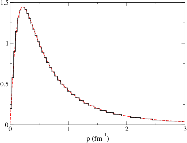
Figure 1: (Color online) Comparison of the exact deuteron wave function obtained in the momentum space for the Yamaguchi potential (dashed curve) with its approximation in the lattice basis (solid line).

The Fig. 2 displays the functions of two pseudostates (with $k=4,8$) obtained in the lattice basis in comparison with the corresponding exact scattering wave packets which can be calculated exactly for the separable Yamaguchi potential. It is interesting to see that although functions of the exact scattering WP’s (16) (dashed lines in the figure) have the logarithmic singularities at the boundaries of the “on-shell” interval (i.e. the one which the state energy belongs to) they are square-integrable as well as the free-motion WP’s.

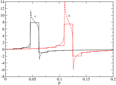
Figure 2: (Color online) The functions of pseudostates ($k=4,8$) obtained in the lattice basis (solid lines) in comparison with exact scattering packets (dashed lines) for the $NN$ spin-triplet Yamaguchi potential.

It is clear from the comparison that the pseudostates composed from step-like wave packets reproduce very well the structure of the exact scattering wave packets “on average”.

Now having at our disposal the two-body bases for subHamiltonians $h_{1}$ and $h_{0}^{1}$ one can construct the three-body WP basis for the channel Hamiltonian $H_{1}$ which defines the asymptotic motion in the system.

II.5 Construction of three-body WP basis for the channel Hamiltonian

The three-body WP states corresponding to the channel Hamiltonian $H_{1}$ can be defined similar as the WP-states for the three-body free Hamiltonian $H_{0}$, i.e. as direct products of two-body WP states for $h_{0}^{1}$ and $h_{1}$ subHamiltonians (jointly with the bound-state) multiplied by the spin functions of the system:

$$|Z^{\Sigma s}_{kj}\rangle\equiv|z_{k}^{s}\rangle\otimes|\mathfrak{q}_{j}\rangle|s,{\frac{1}{2}}:\Sigma\rangle,$$ (19)

where $s$ and $\Sigma$ are the $NN$ subsystem and the total three-body spins correspondingly.

When using the above pseudostate approximation, these three-body states, similarly to two-body scattering WPs, are related to the three-body lattice basis states by a simple rotation transformation (similar to Eq. (18)):

$$|Z_{kj}^{\Sigma s}\rangle=\sum_{i=1}^{M}O_{ki}^{s}|X_{ij}^{\Sigma s}\rangle.$$ (20)

Hence, starting from the free WP bases for every pair subsystem one gets a set of basis states both for the three-body free $H_{0}$ and the channel $H_{1}$ Hamiltonians. The basis defined in Eq. (19) defines an “eigen” WP-subspace for the channel Hamiltonian $H_{1}$.

This allows us to construct an analytical finite-dimensional approximation for the channel resolvent $G_{1}(E)\equiv[E+{\rm i}0-H_{1}]^{-1}$. Indeed, the exact three-body channel resolvent is the convolution of the two-body subresolvents $g_{1}(\varepsilon)$ and $g_{0}^{1}({\cal E})$:

$$G_{1}(E)=\frac{1}{2{\pi\rm i}}\int_{-\infty}^{\infty}{\rm d}\varepsilon g_{1}(\varepsilon)g_{0}^{1}(E-\varepsilon).$$ (21)

Using further the spectral expansions for the two-body resolvents and integrating over $\varepsilon$, one gets an explicit expression for the channel resolvent $G_{1}$ as a sum of two terms $G_{1}(E)=G_{1}^{\rm BC}(E)+G_{1}^{\rm CC}(E)$. Here the bound-continuum part $G_{1}^{\rm BC}(E)$ is the spectral sum over the three-body states corresponding to the free motion of the deuteron relatively to the third nucleon. So, the imaginary part of $G_{1}^{\rm BC}(E)$ is related to a discontinuity on the two-body cut of the Riemann surface of the three-body energy $E$. The continuum-continuum part $G_{1}^{\rm CC}(E)$ of the channel resolvent includes the channel three-body states with the $NN$ pair with interaction in the continuum and ${\rm Im}G_{1}^{\rm CC}(E)$ is defined by a discontinuity on the three-body cut on the energy surface (see the details in Ref. KPR1 ).

Projecting the exact channel resolvent onto the three-body channel WP basis defined in Eq. (19), one can find analytical formulas for the matrix elements of the $G_{1}$ operator. The respective matrix is diagonal in all wave-packet and spin indices:

$$\langle Z_{kj}^{\Sigma s}|G_{1}(E)|Z^{\Sigma s^{\prime}}_{k^{\prime}j^{\prime}}\rangle=\delta_{kk^{\prime}}\delta_{jj^{\prime}}\delta_{ss^{\prime}}G^{\Sigma s}_{kj}(E).$$ (22)

Here the diagonal matrix elements $G_{kj}^{\Sigma s}(E)$ are defined as integrals over the respective momentum bins and depend in general on the spectrum partition parameters (i.e. the $p_{i}$ and $q_{j}$ values) and the total energy $E$ only. They do not depend explicitly on the interaction potential $v_{1}$. If the solution of scattering equations in the finite-dimensional WP basis converges with increasing the basis dimension, the final result turns out to be independent on the particular spectral partition parameters. We have found K2 the explicit formulas for the resolvent matrix elements (22) when one uses the energy WP’s, i.e. WP’s with the weight functions $f(p)=\sqrt{p}$, $w(q)=\sqrt{q}$.

The representation (22) for the channel resolvent is the basic expression for our wave-packet approach, since it gives explicit analytical formulas for the three-body resolvent and thus it allows to simplify drastically the solution of general three-body scattering problem. This expression can be used directly to solve the finite-dimensional analog of the Faddeev equations for the three components of the total scattering wave function KPR2 . Alternatively the very convenient representation (22) can also be used to solve some particular three-body scattering problems using the three-body Lippmann–Schwinger equations KPR1 .

III Solution of $nd$ scattering problem

Now let us proceed with solving the $nd$ elastic and breakup scattering problems.

III.1 The elastic and breakup $nd$ scattering amplitudes

The elastic scattering observables can be found from the Faddeev equation (FE) for the transition operator $\bar{U}$, e.g. in the form Gloeckle_rep :

$$\bar{U}=PG_{0}^{-1}+PtG_{0}\bar{U},$$ (23)

where $t$ is two-body $t$-matrix in three-body space and $P$ is the particle permutation operator. The equivalent form of FE for the transition operator $U$ has the form:

$$U=Pv_{1}+Pv_{1}G_{1}U,$$ (24)

where $G_{1}$ is the resolvent of the channel Hamiltonian $H_{1}$. Since $tG_{0}\equiv v_{1}G_{1}$ the operators $\bar{U}$ and $U$ coincide on-shell and half-shell.

Since the determination of the off-shell channel resolvent in three-body space is a rather time consuming solution of the FE in the form (24), it is very seldom employed for practical solutions. Actually a similar form of the equations is associated with formalisms of the configuration space Faddeev equations, where quite different numerical approaches have been employed Bound_Gl ; Vlach than for the momentum space FE. However, since in the lattice approach one has explicit analytical formulas for the three-body channel resolvent $G_{1}$ the form (24) of FE turns out to be very appropriate for the numerical solution in a WP basis.

The elastic $nd$ scattering amplitude (for a given value of total spin $\Sigma$) can be defined as matrix element of the solution of the Eq. (24) taken in the initial state $|z_{0},q_{0},\Sigma\rangle$:

$$A^{\Sigma}_{\rm el}(q_{0})=\frac{2}{3}\frac{m}{q_{0}}\langle z_{0},q_{0},\Sigma|U|z_{0},q_{0},\Sigma\rangle.$$ (25)

The breakup amplitude for one Faddeev component of the three-body wave function (the so-called single-component amplitude) can be found from the elastic transition operator $U$ after applying the operator $tG_{0}$ from the left:

$$T^{\Sigma s}(p,q)=\frac{\langle p,q,\Sigma s|tG_{0}U|z_{0},q_{0},\Sigma\rangle}{pqq_{0}}.$$ (26)

To obtain the differential breakup cross sections, the total breakup amplitudes can be found by the contributions of all three single-component amplitudes.

Thus, we change the conventional treatment of the breakup process Gloeckle_rep and consider the three-body asymptotic states as scattering states for the channel Hamiltonian $H_{1}$ rather than as the states of the three-body continuum for the free Hamiltonian $H_{0}$. It is a quite natural when treating the elastic scattering amplitudes because the initial state wave functions correspond to the channel Hamiltonian $H_{1}$. In full analogy with this, one can treat the deuteron breakup as its excitation into a continuum $NN$-state in the two-body subsystem governed by the $h_{1}$ subHamiltonian. As was already indicated above such a treatment of breakup processes is close to the configuration space approach.

In fact, when solving the three-body Faddeev equations in the configuration space Bound_Gl ; Vlach ; GPF one finds the breakup amplitude ${\cal A}(\theta)$ which determines the asymptotic behavior of the three-body wave function in hyperspherical coordinates $\rho=\sqrt{x^{2}+\frac{4}{3}y^{2}}$ and $\vartheta=\arctan(\frac{2y}{\sqrt{3}x})$ as follows

$$\psi({\bf x},{\bf y})\xrightarrow[\rho\to\infty]{}\frac{{\cal A}(\theta)}{(K\rho)^{5/2}},\quad K=\sqrt{p^{2}+{\frac{3}{4}}q^{2}},$$ (27)

where $x$ and $y$ are two Jacobi coordinates and $K$ is the hypermomentum.

This breakup amplitude is defined for every spin-angular configuration and interrelated to the partial single-component breakup amplitudes (26) by the following formula

$${\cal A}^{\Sigma s}(\theta)=\frac{4\pi m}{3\sqrt{3}}q_{0}K^{4}e^{i\pi/4}T^{\Sigma s}(p,q),\ \theta=\arctan(\frac{\sqrt{3}q}{2p})$$ (28)

where $\theta$ is the hyperangle in momentum space.

Now if one transforms the formulas for the breakup amplitudes $\cal A$ from Bound_Gl to the integral form one receives the following definition for the breakup amplitudes in the momentum hyperspherical representation

$${\cal A}^{\Sigma s}(\theta)=\frac{4\pi m}{3\sqrt{3}}\frac{K^{4}}{pq}e^{i\pi/4}\langle z_{0},q_{0},\Sigma|U|\phi_{p}^{s(+)},q,\Sigma\rangle,$$ (29)

where $|\phi_{p}^{s(+)}\rangle$ is scattering function for the Hamiltonian $h_{1}$ corresponding to the outgoing boundary condition. These functions are distinguished from the real-valued functions $|\phi_{p}^{\alpha}\rangle$ used in our approach by only a phase factor:

$$|\phi_{p}^{s(+)}\rangle=e^{i\delta_{s}(p)}|\phi_{p}^{s}\rangle,$$ (30)

where $\delta_{s}(p)$ is the s-wave phase shift of the $NN$ scattering in the channel with spin $s$.

Using formulas (29) and (28) one can derive an alternative to formula (26) for the single-component breakup amplitude via the scattering functions of the channel Hamiltonian $H_{1}$

$$T^{\Sigma s}(p,q)={e^{i\delta_{s}(p)}}\frac{\langle z_{0},q_{0},\Sigma|U|\phi_{p}^{s},q,\Sigma\rangle}{pqq_{0}}.$$ (31)

Summarizing this derivation one can conclude that the breakup amplitudes can be defined quite similar to a matrix element for the elastic scattering transition operator $U$ with replacement of the the $NN$ bound-state wavefunction with the exact scattering functions for the $NN$ subHamiltonian.

Having now the required representations for both the elastic and breakup amplitudes, we will proceed in solving the Faddeev equation in “eigen” WP subspace of the channel Hamiltonian $H_{1}$.

III.2 Solution of the Faddeev equation in the three-body WP basis

In our wave-packet approach, all the operators in Eq. (24) are projected onto a three-body wave-packet basis corresponding to the channel Hamiltonian $H_{1}$. In other word, every operator, e.g. $U$, is replaced with its finite-dimensional WP representation:

$$\mathfrak{U}^{\Sigma}=\sum_{s,kj}\sum_{s^{\prime},k^{\prime}j^{\prime}}|Z_{kj}^{\Sigma s}\rangle\langle Z_{kj}^{\Sigma s}|U|Z^{\Sigma s^{\prime}}_{k^{\prime}j^{\prime}}\rangle\langle Z^{\Sigma s^{\prime}}_{k^{\prime}j^{\prime}}|.$$ (32)

Finally one gets the matrix analog for the Eq. (24) (for the given value of $\Sigma$)

$${\mathbb{U}}={\mathbb{P}}{\mathbb{V}}_{1}+{\mathbb{P}}{\mathbb{V}}_{1}{\mathbb{G}}_{1}{\mathbb{U}}.$$ (33)

Here ${\mathbb{V}}_{1}$ and ${\mathbb{G}}_{1}$ are the matrices of the pair interaction and the channel resolvent respectively, the matrix elements of which can be found in an explicit form.

The matrix ${\mathbb{V}}_{1}$ of the potential $v_{1}$ is diagonal in the indices $j,j^{\prime}$ of the wave-packet basis (6) for the free subHamiltonian $h^{0}$ and has the block form:

$$[{\mathbb{V}}_{1}]^{ss^{\prime}}_{kj,k^{\prime}j^{\prime}}=\delta_{jj^{\prime}}\delta_{ss^{\prime}}\langle z_{k}^{s}|v^{s}_{1}|z_{k^{\prime}}^{s}\rangle.$$ (34)

These matrix elements do not depend on in index $j$ and can be written with the usage of the rotation matrix $\mathbb{O}$ defined in Eq. (18) as:

$$\langle z_{k}^{s}|v^{s}_{1}|z_{k^{\prime}}^{s}\rangle=\sum_{i,i^{\prime}}O_{ki}^{s}O_{k^{\prime}i^{\prime}}^{s}\langle\mathfrak{p}_{i}^{s}|v^{s}_{1}|\mathfrak{p}_{i^{\prime}}^{s}\rangle.$$

In the last expression, the potential matrix elements in the free WP basis are used which have the form

$$\langle\mathfrak{p}_{i}^{s}|v^{s}_{1}|\mathfrak{p}_{i^{\prime}}^{s}\rangle=\frac{1}{\sqrt{d_{i}d_{i^{\prime}}}}\int_{\mathfrak{D}_{i}}dp\int_{\mathfrak{D}_{i^{\prime}}}dp^{\prime}\ {v_{1}^{s}(p,p^{\prime})}$$ (35)

where $v_{1}^{s}(p,p^{\prime})$ is the momentum representation for the interaction potential. It implies that the matrix elements (III.2) can be found analytically for a wide variety of the potential forms.

An important ingredient of our lattice approach presented here is the representation of the permutation operator $P$ as an overlap matrix $\mathbb{P}$ between the channel WP basis functions for different sets of the Jacobi coordinates. Using further the approximation (18) for the scattering wave packets $|z_{k}^{s}\rangle$, these matrix elements can be expressed through the overlap matrix ${\mathbb{P}}^{0}$ for the free lattice basis function of Eq. (15) with the help of the rotation matrices $\mathbb{O}$

$$\langle Z_{kj}^{\Sigma s}|P|Z_{k^{\prime}j^{\prime}}^{\Sigma s^{\prime}}\rangle\approx\sum_{ii^{\prime}}O_{ki}^{s}O_{k^{\prime}i^{\prime}}^{s^{\prime}*}\langle X_{ij}^{\Sigma s}|P|X_{i^{\prime}j^{\prime}}^{\Sigma s^{\prime}}\rangle.$$ (36)

Now let’s replace the exact operator $U$ in the formula for the elastic $nd$ scattering amplitude (25) with its lattice counterpart $\mathfrak{U}^{\Sigma}$, and employ further the projection rule for the free WP states (11). Then one gets that the on-shell elastic amplitude in the wave-packet representation can be calculated as a a diagonal (on-shell) matrix element of the $\mathbb{U}$-matrix:

$$A_{\rm el}^{\Sigma}(E)\approx\frac{2m}{3q_{0}}\frac{\langle Z^{\Sigma 1}_{0j_{0}}|\mathfrak{U}^{\Sigma}|Z^{\Sigma 1}_{0j_{0}}\rangle}{\bar{d}_{j_{0}}},\quad\Sigma={\frac{1}{2}},{\frac{3}{2}},$$ (37)

where $|Z^{\Sigma 1}_{0j_{0}}\rangle$ is the WP basis state corresponding to the initial state: index 0 denotes the bound state of the $NN$ pair (deuteron) and index $j_{0}$ denotes the “on-shell” $q$-bin $\bar{\mathfrak{D}}_{j_{0}}$ with the on-shell momentum $q_{0}=\sqrt{\frac{4}{3}m(E-\varepsilon_{0}^{*})}$: $q_{0}\in\bar{\mathfrak{D}}_{j_{0}}$.

It has been shown above that the breakup amplitude is proportional to a half-shell matrix element $\langle z_{0},q_{0},\Sigma|U|\phi_{p}^{s},q,\Sigma\rangle$. Substituting, similarly to the calculation of the elastic scattering amplitude, the finite-dimensional operator $\mathfrak{U}^{\Sigma}$ into the expression for the breakup amplitude and utilizing the projection rules for the free-motion and scattering wave-packets, one gets:

$$T^{\Sigma s}(p,q)\approx e^{i\delta(p^{*}_{k})}\frac{{\mathbb{T}}^{\Sigma s}_{0j_{0},kj}}{p_{k}^{*}q_{j}^{*}q_{0}},$$

$${\mathbb{T}}^{\Sigma s}_{0j_{0},kj}\equiv\frac{\langle Z^{\Sigma 1}_{0j_{0}}|\mathfrak{U}^{\Sigma}|Z^{\Sigma s}_{kj}\rangle}{\sqrt{\bar{d}_{j_{0}}D_{k}^{s}\bar{d}_{j}}},\quad\begin{array}[]{c}q_{0}\in\bar{\mathfrak{D}}_{j_{0}},\\ q\in\bar{\mathfrak{D}}_{j},\\ p\in\Delta_{k}^{s},\\ \end{array}$$ (41)

where $p_{k}^{*}=\sqrt{2m\varepsilon_{k}^{*s}}$ and $q^{*}_{j}={\frac{1}{2}}[q_{j-1}+q_{j}]$ are momenta corresponding to $\Delta_{k}^{s}$ and $\bar{\mathfrak{D}}_{j}$ bins respectively and the $D_{k}^{s}$ is the momentum width of the $\Delta_{k}^{s}$ bin.

Thus, we just have found that the elastic and breakup amplitudes can be calculated directly using the diagonal (“on-shell”) and non-diagonal (“half-shell”) matrix elements of the same operator $\mathfrak{U}^{\Sigma}$.

However, some problem still arises here: how to define correctly which of the basis states $Z_{kj}^{\Sigma s}$ correspond to the on-shell states of the $H_{1}$. Due to the discretization of the spectrum every WP basis state corresponds to the energy $E_{kj}^{s}=\varepsilon_{k}^{s*}+{\cal E}_{j}^{*}$ and thus one does not get the exact coincidence of these energies for different “on-shell” three-body WP states with the energy $E$ of the initial state. In other words, the energy conservation for three-body WP states is fulfilled only approximately within the corresponding bin widths. To avoid this difficulty we apply some energy averaging procedure to the transition matrix elements which is quite natural for the lattice-like representation.

III.3 The energy averaging procedure for the breakup amplitudes.

Let us to rewrite expression (31) for the breakup amplitude via wave functions of pair subsystems normalized to $\delta$-functions in energy. Then, when calculating the breakup amplitudes one will need the transition operator matrix elements of the form (we omit for the sake of brevity all the spin labels):

$$u(E,\varepsilon)=\langle z_{0},\psi_{0}(E-\varepsilon_{0}^{*})|{U}|\phi(\varepsilon)\psi_{0}(E-\varepsilon)\rangle,$$ (42)

where $|\phi(\varepsilon)\rangle$ is the $NN$ scattering state with energy $\varepsilon$, $|\psi_{0}(E-\varepsilon)\rangle$ is the wave function of the subHamiltonian $h_{0}^{1}$ describing the free motion of the third nucleon relative to the $NN$ subsystem, and $E$ is the total energy in the c.m. system. In the framework of the fully-discretized representation it is quite natural to make an energy averaging for the transition matrix elements $u(E,\varepsilon)$ over the excitation energy $\varepsilon$, which leads to the following integrals:

$$u_{n}(E)\equiv\frac{1}{\Delta_{n}}\int_{\varepsilon_{n-1}}^{\varepsilon_{n}}d\varepsilon\langle z_{0},\psi_{0}(E-\varepsilon_{0}^{*})|U|\phi(\varepsilon)\psi_{0}(E-\varepsilon)\rangle,$$ (43)

here $\{[\varepsilon_{n-1},\varepsilon_{n}]\}$ is some set of intervals, in general independent of the initial partition of the excitation energy $\varepsilon$. $\Delta_{n}=\varepsilon_{n}-\varepsilon_{n-1}$ are the corresponding widths.

Further, by replacing the exact $U$ operator with its wave packet counterpart (32) and using the projection rules for the scattering and free WP’s, one can define a new approximation for the breakup amplitudes:

$${\mathbb{T}}^{\Sigma s}_{n}(E)=\sum_{kj}{\mathbb{T}}^{\Sigma s}_{0j_{0},kj}\frac{1}{\Delta_{n}}\big{[}\min(\varepsilon_{n},\varepsilon_{k},E-{\cal E}_{j-1})-$$ (44)

$$-\max(\varepsilon_{n-1},\varepsilon_{k-1},E-{\cal E}_{j})\big{]}.$$

Here the sum runs over all possible indices $k$ and $j$ for which the difference in the square brackets is positive.

Then, for the single-component breakup amplitudes, one obtains the following approximate expression with the elements ${\mathbb{T}}_{n}$:

$$T^{\Sigma s}(p_{n}^{*},q_{n}^{*})\approx e^{i\delta(p^{*}_{n})}\frac{{\mathbb{T}}_{n}^{\Sigma s}}{p_{n}^{*}q_{n}^{*}q_{0}},\quad\begin{array}[]{l}p_{n}^{*}=\sqrt{{m\varepsilon_{n}^{*}}},\\ q_{n}^{*}=\sqrt{{\frac{4}{3}}m(E-\varepsilon_{n}^{*})},\\ \varepsilon_{n}^{*}={\frac{1}{2}}[\varepsilon_{n-1}+\varepsilon_{n}].\end{array}$$ (45)

Now, using the energy averaged WP amplitudes one can get easily the following formula for the breakup amplitude in the hyperspherical representation:

$${\cal A}_{n}^{\Sigma s}(\theta)=\frac{4\pi m}{3\sqrt{3}}\frac{K^{4}}{p_{n}^{*}q_{n}^{*}}e^{i\delta(p^{*}_{n})}{\mathbb{T}}^{\Sigma s}_{n},\quad\cos\theta=\sqrt{\frac{\varepsilon_{n}^{*}}{E}}.$$ (46)

III.4 Breakup differential cross section

After the determination of the single-component breakup amplitudes, the total breakup amplitude is derived using contributions of all three Faddeev components and can be written with the help of the particle permutation operator $P$ in the following way:

$$A_{\rm br}^{\rm tot}({\bf p},{\bf q};{\bf q}_{0})=\langle{\bf p},{\bf q}|(1+P)tG_{0}U|z_{0},{\bf q}_{0}\rangle.$$ (47)

The differential breakup cross section is related to this total breakup amplitudes as follows Gloeckle_rep :

$$\frac{d^{5}\sigma}{d{\bf\hat{k}}_{1}d{\bf\hat{k}}_{2}dS}=(2\pi)^{4}\frac{2m}{3q_{0}}\bar{k}_{S}|A_{\rm br}^{\rm tot}({\bf p},{\bf q};{\bf q}_{0})|^{2}.$$ (48)

Here ${\bf k}_{1}$ and ${\bf k}_{2}$ are momenta of particles to be registered, $S$ is the arclength of the kinematical curve and $\bar{k}_{S}$ is the phase space volume defined as:

$$\bar{k}_{S}=\frac{m^{2}k_{1}k_{2}}{\sqrt{\left(\frac{2k_{2}-{\bf\hat{k}}_{2}({\bf k}_{\rm lab}-{\bf k}_{1})}{k_{2}}\right)^{2}+\left(\frac{2k_{1}-{\bf\hat{k}}_{1}({\bf k}_{\rm lab}-{\bf k}_{2})}{k_{1}}\right)^{2}}},$$ (49)

where ${\bf k}_{\rm lab}={\frac{3}{2}}{\bf q}_{0}$ is the center of mass momentum in the laboratory system.

In the case of $s$-wave $NN$ interactions, the total breakup amplitude is defined as sum of spin-quartet ($\Sigma={\frac{3}{2}}$) and spin-doublet ($\Sigma={\frac{1}{2}}$) single-component terms defined for all different Jacobi sets. E. g. the $S$-wave amplitude of the two-neutron emission can be represented as a sum of three terms

$$|A_{\rm br}^{\rm tot}|^{2}=(2|M^{{\frac{3}{2}}1}|^{2}+|M^{{\frac{1}{2}}0}|^{2}+|M^{{\frac{1}{2}}1}|^{2})/3,$$ (50)

where $M^{\Sigma s}$ are the total amplitudes for the quartet and doublet channels. In accordance with Ref. Cahill , they are expressed through single-component breakup amplitudes defined for different sets of Jacobi momenta $(p_{a},q_{a})$ as follows (we assume here that neutrons are particles 1 and 2 and the proton is the particle 3):

$$\begin{array}[]{ll}M^{{\frac{3}{2}}1}=&T^{{\frac{3}{2}}1}(p_{1},q_{1})-T^{{\frac{3}{2}}1}(p_{2},q_{2}),\\ M^{{\frac{1}{2}}0}=&\frac{2}{\sqrt{3}}\Big{\{}\frac{1}{4}[T^{{\frac{1}{2}}0}(p_{1},q_{1})+T^{{\frac{1}{2}}0}(p_{2},q_{2})]-\\ &{\frac{3}{4}}[T^{{\frac{1}{2}}1}(p_{1},q_{1})+T^{{\frac{1}{2}}1}(p_{2},q_{2})]+T^{{\frac{1}{2}}0}(p_{3},q_{3})\Big{\}},\\ M^{{\frac{1}{2}}1}=&\frac{1}{2}\Big{\{}T^{{\frac{1}{2}}0}(p_{1},q_{1})-T^{{\frac{1}{2}}0}(p_{2},q_{2})+\\ &T^{{\frac{1}{2}}1}(p_{1},q_{1})-T^{{\frac{1}{2}}1}(p_{2},q_{2})\Big{\}}.\\ \end{array}$$ (51)

Finally the differential cross section of the $n-d$ breakup is expressed through the partial total amplitude (50) as:

$$\frac{d^{5}\sigma}{d\hat{k}_{1}d\hat{k}_{2}dS}=\frac{\pi}{4}\frac{2m}{3q_{0}}\bar{k}_{S}|A_{\rm br}^{\rm tot}|^{2}.$$ (52)

To determine the differential cross section for the two-neutron emission one has to calculate the elements ${\mathbb{T}}_{n}$ (44) for every spin component $(\Sigma s)$ of the total breakup amplitude and then substitute them into the explicit formulas (51) and (50).

Thus, it has been demonstrated above that in our WP approach one can find quite naturally all breakup amplitudes together with the elastic scattering amplitude. This gives a very nice universal and unified calculation scheme. Some details of the numerical procedure for solving the matrix equation (33) are discussed in Appendix C.

IV Illustrative examples

Because we have developed here a novel approach for the treatment of the three-body breakup processes we would need precise and reliable tests to check our new procedure. In all the tests below we employ as a convenient universal WP basis the free momentum wave packets for Jacobi momenta $q$ and $p$ constructed using the generalized Tchebyshev grid:

$$q_{i}=q_{\rm m}\left[\tan\left(\frac{i}{2N+1}\pi\right)\right]^{t},i=1,\ldots,N,$$ (53)

where $q_{\rm m}$ is the common scale parameter and the $t$-parameter determines the “sparseness degree” of the bin set. A similar grid with the size $M$ and common scale $p_{\rm m}$ is introduced for discretization of the momenta $p$.

IV.1 $nd$ breakup amplitudes for a separable $NN$ potential

As a first extremely convenient test we have chosen the three-body model with a separable $NN$-potential. This model, which can be treated numerically very accurately in various kinematical breakup situations seems to be very appropriate for such a test (see below).

We consider here the $nd$ breakup with pairwise separable $NN$-interactions in the form:

$$v^{s}=\lambda_{s}|\varphi_{s}\rangle\langle\varphi_{s}|,\quad s=0,1$$ (54)

As it is well known, the Faddeev equations for such potentials can be reduced to one-dimensional integral equations in momentum space. Such equations, as demonstrated in our previous work KPR1 , can be solved quite accurately using the two-body free WP basis. For convenience of the reader we describe all the details of this procedure in Appendix B. Here we will refer to the results found in such approach as to the “exact ones”. We will compare the latter with the results of the solution of the general three-body WP scheme with the Eq. (33) for the separable potential.

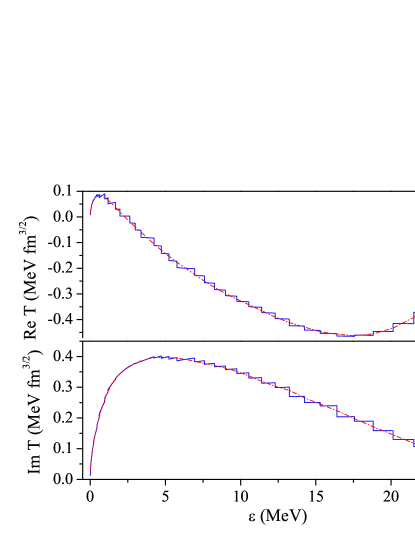
Figure 3: (Color online) Comparison of the energy unaveraged (solid curve) and averaged (dashed-dotted curve) breakup amplitudes ${\mathbb{T}}^{{\frac{3}{2}}1}$ for the separable $NN$ potential (54) calculated with the general WP technique at the basis size $M=N=100$ .

The Fig. 3 shows the unaveraged (i.e. having a histogram form) and energy averaged breakup amplitudes for the Yamaguchi potential obtained from the general matrix FE (33) in the lattice basis. The energy averaged amplitudes have been calculated using the averaging procedure described above. It is clearly seen from Fig. 3 the method developed makes it possible to find rather smooth energy dependence for the breakup amplitudes. Using the averaged amplitudes, we have found the single-component breakup amplitudes ${\mathbb{T}}^{\Sigma s}$ as functions of hyperangle $\theta$ for both quartet and doublet three-body spin channels.

Now, we can compare the approximated WP breakup amplitudes (44) found within our general formalism for a separable model with the exact amplitudes derived from directly solving the one-dimensional Faddeev equations. In the Figs. 4-6 such a comparison between approximated and “exact” results is presented. The two-body free WP bases with size $M=200$ and $N=200$ have been used in the calculation of the approximated amplitudes.

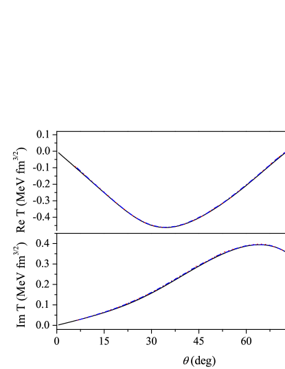
Figure 4: (Color online) The breakup amplitude $\mathbb{T}^{{\frac{3}{2}}1}$ in the quartet channel calculated for the separable $NN$ potential via the general WP technique for basis dimensions $M=N=100$ (dotted curves) and $M=N=200$ (dash-dotted curves) in comparison with the ’exact’ values (full curves). with the resolution of this figure the three curves can practically not be distinguished.

We observe in the Figs. 4-6 quite a very good agreement between the lattice-approximations and the “exact” amplitudes. The corresponding curves are almost indistinguishable in the figures. The only differences are seen at the hyperangle region $\theta\sim$ 90^∘ for the spin-doublet $T^{{\frac{1}{2}}0}$ amplitude. It is clear also that the WP amplitudes calculated in a finite-dimensional $L_{2}$ basis converge to the exact ones with increasing basis size.

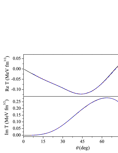
Figure 5: (Color online) The breakup amplitude $\mathbb{T}^{{\frac{1}{2}}1}$ in the spin-doublet channel for a separable $NN$ model. The notations are the same as in the Fig. 4.

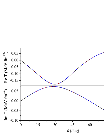
Figure 6: (Color online) The breakup amplitude $\mathbb{T}^{{\frac{1}{2}}0}$ in the spin-doublet channel for the separable $NN$-model. The notations are the same as in the Fig. 4.

IV.2 n-d breakup amplitudes for a local NN potential

Having tested our novel approach using the simple separable model for the $NN$ force one can move to a more realistic case of a local $NN$-interaction. For this, we have chosen the so-called MT I-III $NN$ central potential which was frequently used in the past for the test of few-body calculations. So, we can compare our results for this model with very accurate benchmark calculations Friar . For the present WP calculations we use again the three-body lattice basis constructed on a Tchebyshev two-dimensional grid.

The results of such a comparison are presented in Fig. 7-9 for our single-component hyperspherical amplitudes ${\cal A}^{\Sigma s}$. One can observe in the Figs. 7-9 a quite satisfactory general agreement with the results of the benchmark calculations Friar except in the region $\theta\sim$ 90^∘, similarly to the case of the separable $NN$ interaction. It should be mentioned, that the from the amplitude ${\cal A}$ Eq. (46) has an additional factor inversely proportional to the relative momentum $p$ compared to the amplitude $\mathbb{T}$ discussed in the previous subsection. So, the differences to the exact solution of ${\cal A}$ are more visible at the region corresponding to small values of $p$.

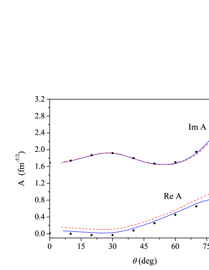
Figure 7: (Color online) The breakup amplitudes ${\cal A}^{{\frac{3}{2}}1}$ in the spin-quartet channel calculated using the WP technique for the $NN$ force MT I-III for basis size $M=N=100$ (dashed curves) and $M=N=200$ (solid curves) in comparison with the results of the benchmark calculations (solid circles) Friar .

Similar difficulties at $\theta\sim$ 90^∘ are also observed in other works Bound_Gl ; Vlach ; GPF in which the breakup calculations have been done in the configuration space. In Ref. GPF it has been demonstrated that for the correct calculation of the breakup amplitudes in the area of small relative $NN$ momenta one has to employ the explicit integral form for the breakup amplitude $T(p,q)$.

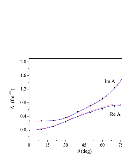
Figure 8: (Color online) The breakup ${\cal A}^{{\frac{1}{2}}1}$ amplitudes in spin-doublet channel for the MT I-III $NN$ potential. The notations are the same as in Fig. 7.

In our approach the minor disagreement of the WP breakup amplitudes and the exact benchmark results at very low relative momenta can be related to some uncertainties in the determination of the widths and the corresponding values of momenta for the WP scattering states of the pair continuum very close to the threshold. So the case of very low relative momenta in the lattice approach deserves a separate study which is under way.

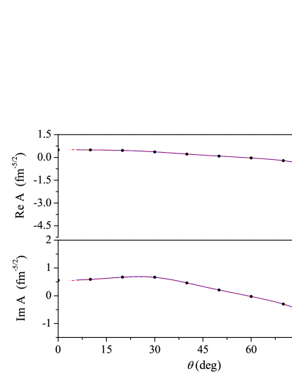
Figure 9: (Color online) The breakup amplitudes ${\cal A}^{{\frac{1}{2}}0}$ in the spin-doublet channel for the MT I-III $NN$ force. The notations are the same as in Fig. 7.

Using further the single-component amplitudes we have found the total (i.e. with inclusion of all three Faddeev components) breakup amplitudes as well as differential cross sections of two-neutron emission for different kinematical configurations. In Figs. 10 and 11 the differential cross sections for two-neutron emission with our WP technique are presented for two configurations and compared to the results of Ref. Friar . One configuration includes the FSI peak while the second one is related to the so called “space-star” breakup kinematics. For derivation of the Faddeev cross sections we used an interpolation of the data in the table presented in Ref. Friar for the single-component amplitudes.

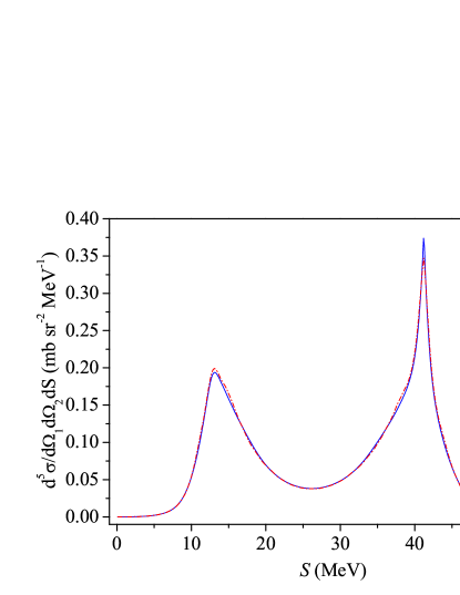
Figure 10: (Color online) The differential cross section for two-neutron emission at the kinematical configuration: $\theta_{1}=45^{\circ}$, $\theta_{2}=50.64^{\circ}$, $\phi_{12}=180^{\circ}$ at the incident neutron energy $E_{\rm lab}=42$ MeV found with usage of the WP technique (dotted curve) and the conventional Faddeev calculations (solid curve). (”Final state peak”.)

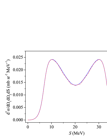
Figure 11: (Color online) The same as in the Fig. 10 but for the kinematical configuration $\theta_{1}=53.6^{\circ}$, $\theta_{2}=53.6^{\circ}$, $\phi_{12}=120^{\circ}$. (”Space star”.)

In summary, the agreement between conventional and lattice results is generally very good. The curves are mostly hardly distinguishable in Figs. 10,11.

V Summary

In the present work we generalized the wave-packet method developed by the present authors earlier for the discretization of the three-body continuum and used it for finding the three-body breakup amplitudes. As far as the present authors are aware, the study in the work is the first where the Faddeev breakup amplitudes are obtained completely in the three-body $L_{2}$-basis. Thus, it would be appropriate to enumerate some important distinctive features of our lattice-like approach.

1. Due to projection of the scattering integral equations onto the wave-packet $L_{2}$ basis corresponding to the three-body channel Hamiltonian $H_{1}$, we get an explicit analytical representation for the three-body channel resolvent $G_{1}$ that is used in all further calculations. For this we employ the version of the integral Faddeev equations with the kernel $Pv_{1}G_{1}$ instead of the conventional form $Pt_{1}G_{0}$. This simplifies drastically the whole calculations scheme as compared to the conventional one, because first we do not need to know the full off-shell pair $t$-matrix at many different energies and in addition we get the matrix kernel in a very convenient finite-dimensional form. As an input information for the $NN$-interaction, we use only the results of a single diagonalization (for every spin channel) of the $NN$ Hamiltonian matrix. From such a diagonalization we get immediately the whole set of pseudo-states (the scattering WP’s) and partial phase shifts at many energies corresponding to these pseudo-states KPRF .

2. For the matrix of the transition operator, one gets an universal linear matrix equation with finite matrix elements. The diagonal (on-shell) elements of this solution determines the elastic scattering amplitudes while the non-diagonal (half-shell) elements determines the single-component breakup amplitudes up to some known phase factor.

3. The structure of the kernel for the matrix equation obtained is very convenient for numerical realization. Due to the fact that the kernel is a product of a diagonal matrix, two block matrices and a very sparse matrix, it is possible to greatly reduce requirements for the RAM storage size and noticeably decrease the computation time.

4. The effect of the particle permutation operator in the Faddeev kernel is represented now with the help of the universal matrix of basis functions overlapping for different Jacobi coordinate sets. It allows to avoid very time-consuming numerous re-interpolations of the current solutions (at iterations) from one set of Jacobi coordinates to another one at every iteration step Gloeckle_rep .

5. Due to an averaging of the integral kernels over the cells in momentum space the very complicated energy singularities of the kernel above the breakup threshold (e.g. the moving branching points etc.) are smoothed and one can solve the few-body scattering equations directly at real energies, i.e. without any contour deformation to the complex-energy plane. This fact also facilitates enormously the practical solution of few-body equations above the breakup threshold.

6. The comparison of the results obtained in our approach with those for the model for the separable $NN$ potential and with benchmark breakup calculations (with a semi-realistic local $NN$-potential) has demonstrated that the WP method allows to get quite accurate three-body breakup amplitudes and cross sections. Still, the region of very low relative $NN$ momenta requires some additional study. Some inaccuracy of our results in this area can be related to two factors: (i) a slow convergence of the WP amplitudes in this region, and (ii) some uncertainty of the WP representation of the two-body continuum in the region of very low relative momenta. We plan to devote a special study for the solution of this problem.

In summary one can conclude that the total lattice-like $L_{2}$ discretization of the three-body continuum allows to find an accurate solution for the three-body Faddeev equations for breakup amplitudes and simplifies enormously the calculation together with a noticeable reduction of the computational cost.

Acknowledgments The authors appreciate a partial financial support from the RFBR grants 10-02-00096, 10-02-00603, and 12-02-00908.

Appendix A The permutation matrix in the lattice basis

In our approach we employ a lattice basis, i.e. a basis built by free WP’s in momentum space. The two-dimensional (three-body) wave packet in momentum space are step-like functions of variables $p$ and $q$:

$$\langle p,q|\mathfrak{p}_{i}\mathfrak{q}_{j}\rangle\equiv\langle p,q|\mathfrak{D}_{ij}\rangle=\frac{1}{\sqrt{d_{i}\bar{d}_{j}}}{\vartheta(p\in\mathfrak{D}_{i})}{\vartheta(q\in\bar{\mathfrak{D}}_{j})},$$ (55)

which are nonzero only at the intervals $\mathfrak{D}_{i}=[p_{i-1},p_{i}]$ and $\bar{\mathfrak{D}}_{j}=[q_{j-1},q_{j}]$ ($d_{i}$ and $\bar{d}_{j}$ are the widths of corresponding intervals). Such wave packets are normalized to unity with the weight $dpdq$ and form an orthonormal basis (it is assumed that the intervals are not overlapping).

The matrix element of the permutation operator $P$ between plane waves has a simple form for the $s$-wave:

$$\langle p^{\prime},q^{\prime},s^{\prime}\Sigma|P|p,q,s\Sigma\rangle\equiv\Lambda^{\Sigma}_{s^{\prime}s}P^{0}(p^{\prime},q^{\prime},p,q)=$$

$$\Lambda^{\Sigma}_{s^{\prime}s}\ {4}\delta({p^{\prime}}^{2}+{\frac{3}{4}}{q^{\prime}}^{2}-(p^{2}+{\frac{3}{4}}q^{2}))\,\vartheta(1-|x|),$$ (56)

where $\Lambda^{\Sigma}_{ss^{\prime}}$ is a spin-channel coupling matrix. The $\delta$-function guaranties energy conservation and $x$ is the cosine of the angle between vectors $\bf q$ and $\bf q^{\prime}$ which (with taking into account the $\delta$-function) can be expressed as a function of three momenta, e.g. $p$, $q$, $q^{\prime}$:

$$x=\frac{p^{2}-{q^{\prime}}^{2}-q^{2}/4}{qq^{\prime}}.$$ (57)

The condition $|x|<1$ in (A) restricts the allowed values of momenta to a region, where the overlap is nonzero.

To find the matrix elements of the permutation operator $P$ over the free WPs (55), one has to integrate the function $P^{0}(p^{\prime},q^{\prime},p,q)$ over rectangular cells $\mathfrak{D}_{ij}=\mathfrak{D}_{i}\otimes\bar{\mathfrak{D}}_{j}$, $\mathfrak{D}^{\prime}_{i^{\prime}j^{\prime}}=\mathfrak{D}^{\prime}_{i^{\prime}}\otimes\bar{\mathfrak{D}}^{\prime}_{j^{\prime}}$ (where the upper prime at the interval symbol denote that it refers to a different set of Jacobi coordinates):

$$\langle\mathfrak{D}^{\prime}_{i^{\prime}j^{\prime}}|P|\mathfrak{D}_{ij}\rangle=\frac{1}{\sqrt{d_{i}\bar{d}_{j}d_{{i^{\prime}}}\bar{d}_{{j^{\prime}}}}}\times$$ (58)

$$\int_{\mathfrak{D}^{\prime}_{i^{\prime}j^{\prime}}}\int_{\mathfrak{D}_{ij}}P^{0}(p^{\prime},q^{\prime},p,q)\,dp\,dq\,dp^{\prime}\,dq^{\prime}.$$

Actually, the integral in Eq. (58) is reduced to an area of two overlapping rectangular areas $\mathfrak{D}_{ij}$ and $\mathfrak{D}^{\prime}_{i^{\prime}j^{\prime}}$.

Hyperspherical (polar in the s-wave case) coordinates are most convenient to calculate such overlaps. Let us introduce the reduced (rescaled) momentum variable $\tilde{q}$:

$$\tilde{q}=\sqrt{(3/4)}q,$$ (59)

then, the energy conservation takes the “homogeneous” form $p^{2}+\tilde{q}^{2}={p^{\prime}}^{2}+{\tilde{q}}^{{}^{\prime}2}$. The hyperspherical coordinates $Q,\alpha$ are introduced as usually:

$$\tilde{q}=Q\sin\alpha,\quad p=Q\cos\alpha,\quad Q^{2}=p^{2}+\tilde{q}^{2}.$$ (60)

In these hyperspherical coordinates the integral in Eq. (58) takes the following form:

$$\int\delta({p^{\prime}}^{2}+{\frac{3}{4}}{q^{\prime}}^{2}-(p^{2}+{\frac{3}{4}}q^{2}))\vartheta(1-|x|)\,dp\,dq\,dp^{\prime}\,dq^{\prime}$$

$$=(4/3)\int\delta(Q^{2}-{Q^{\prime}}^{2})\vartheta(1-|x|)\,QdQd\alpha Q^{\prime}dQ^{\prime}d\alpha^{\prime}$$

$$=1/3\Pi(\mathfrak{D}_{ij},\mathfrak{D}^{\prime}_{i^{\prime}j^{\prime}}),$$ (61)

where we define the overlapping square:

$$\Pi(\mathfrak{D}_{ij},\mathfrak{D}^{\prime}_{i^{\prime}j^{\prime}})\equiv\int\vartheta(1-|x|)\,d(Q^{2})d\alpha d\alpha^{\prime}.$$ (62)

Thus we get that the permutation matrix element is directly interrelated to this square:

$$\langle\mathfrak{D}^{\prime}_{i^{\prime}j^{\prime}}|P|\mathfrak{D}_{ij}\rangle=\frac{4}{3}\frac{\Pi(\mathfrak{D}_{ij},\mathfrak{D}^{\prime}_{i^{\prime}j^{\prime}})}{\sqrt{d_{i}\bar{d}_{j}d_{i^{\prime}}\bar{d}_{j^{\prime}}}}.$$ (63)

The condition $|x|<1$ can be expressed through the hyperangular variables $\alpha,\alpha^{\prime}$ as follows:

$$|\frac{\pi}{3}-\alpha|<\alpha^{\prime}<\frac{\pi}{2}-|\alpha-\frac{\pi}{6}|$$ (64)

So, the overlap region $S(\alpha,\alpha^{\prime})$ determined by the condition $|x|<1$ is a rectangle in the plane $(\alpha,\alpha^{\prime})$ restricted by four straight lines (see Fig. 12):

Figure 12: The integration region in the plane ($\alpha,\alpha^{\prime}$) which is the intersection of the area of allowable values of $\alpha,\alpha^{\prime}$ — the large rectangle $S$ determined by the inequalities (64) — and the rectangle $R(Q)$ which boundaries depend on the value of $Q$.

Therefore, the integral in Eq. (61) can be evaluated as the external (numerical) integral over $Q^{2}$ in the range between $Q^{2}_{\rm min}$ and $Q^{2}_{\rm max}$ from the area of intersection of the rectangle $S$ and the rectangle $R(\alpha_{\rm min},\alpha_{\rm max},\alpha^{\prime}_{\rm min},\alpha^{\prime}_{\rm max})$ whose vertices depend on $Q$ (see Fig. 12):

$$\Pi=\int_{Q^{2}_{\rm min}}^{Q^{2}_{\rm max}}d(Q^{2})\int\int_{S\cap R(Q)}d\alpha d\alpha^{\prime}.$$ (65)

The integration limits over $Q^{2}$ are equal:

$$Q^{2}_{\rm min}=\max(p_{i-1}^{2}+\tilde{q}_{i-1}^{2},{p^{\prime}}_{j-1}^{2}+(\tilde{q}^{\prime}_{j-1})^{2}),$$ (66)

$$Q^{2}_{\rm max}=\min(p_{i}^{2}+\tilde{q}_{i}^{2},{p^{\prime}}_{j}^{2}+(\tilde{q}^{\prime}_{j})^{2}).$$ (67)

If $Q^{2}_{\rm max}<Q^{2}_{\rm min}$ then the cells do not overlap and the matrix element is equal to 0.

Figure 13: On the definition of the integration limits (66) - (69) in the variables $Q,\alpha,\alpha^{\prime}$. The cells $\mathfrak{D}_{ij}$ and $\mathfrak{D}^{\prime}_{ij}$ in the plane ($p,\tilde{q}$) and their polar coordinates $(\alpha_{\rm min},\alpha_{\rm max})$ and $(\alpha^{\prime}_{\rm min},\alpha^{\prime}_{\rm max})$ are shown.

The coordinates of vertices of the rectangle $R(Q)$ are computed directly (see the Fig. 13 for further explanations):

$$\alpha_{\rm min}(Q)=\max(\arcsin\frac{\tilde{q}_{i-1}}{Q},\arccos\frac{p_{i}}{Q});$$

$$\alpha_{\rm max}(Q)=\min(\arcsin\frac{\tilde{q}_{i}}{Q},\arccos\frac{p_{i-1}}{Q});$$ (68)

$$\alpha^{\prime}_{\rm min}(Q)=\max(\arcsin\frac{\tilde{q}^{\prime}_{j-1}}{Q},\arccos\frac{p^{\prime}_{j}}{Q});$$

$$\alpha^{\prime}_{\rm max}(Q)=\min(\arcsin\frac{\tilde{q}^{\prime}_{j}}{Q},\arccos\frac{{p^{\prime}}_{j-1}}{Q}).$$ (69)

Here, if $p_{i}>Q$ then $\arccos\frac{p_{i}}{Q}$ should be replaced by 0, and if $\tilde{q}_{i}>Q$ then $\arcsin\frac{\tilde{q}_{i}}{Q}$ should be replaced by $\pi/2$; the same rule should be applied also to primed values.

The area of intersection $S\cap R(Q)$ in the plane $\alpha,\alpha^{\prime}$ is evaluated analytically by the formulas of elementary geometry.

Appendix B Wave-packet solution for the three-body scattering problem with a separable potential

We consider here a system of three nucleons with equal masses $m$ interacting by a separable $NN$ force in s-wave spin-singlet ($s=0$) and spin-triplet ($s=1$) states correspondingly:

$$v_{s}=\lambda_{s}|\varphi_{s}\rangle\langle\varphi_{s}|,\quad s=0,1.$$ (70)

The two-body $t$-matrices are also separable:

$$t_{s}(E)=|\varphi_{s}\rangle\tau_{s}(E)\langle\varphi_{s}|,$$ (71)

where $\tau$ are known functions

$$\tau^{-1}_{s}(E)=\lambda_{s}^{-1}-\langle\varphi_{s}|g_{0}(E)|\varphi_{s}\rangle,$$ (72)

and $g_{0}(E)$ is the free two-particle resolvent. Function $\tau_{1}$ for triplet state has the pole at the deuteron binding energy $\varepsilon_{0}^{*}$. The corresponding bound state wavefunction $|z_{0}\rangle$ is defined as follows:

$$|z_{0}\rangle=\sqrt{R(\varepsilon_{0}^{*})}g_{0}(\varepsilon_{0}^{*})|\varphi_{1}\rangle,$$ (73)

where $R(\varepsilon_{0}^{*})$ is the residue of $\tau_{t}(E)$ at the pole.

We use here the two-parameter Yamaguchi potentials with the form factors:

$$\varphi_{s}({p})=(p^{2}+\beta_{s}^{2})^{-1}.$$ (74)

In this case $\tau_{s}(E)$ and $R(\varepsilon_{0}^{*})$ take the form:

$$\tau^{-1}_{s}=\left(\lambda_{s}^{-1}+\frac{\pi m}{\beta_{s}}\frac{1}{(\beta_{s}-i\sqrt{mE})^{2}}\right),$$

$$R(\varepsilon_{0}^{*})=\frac{\beta_{1}(b^{2}+p_{b}^{2})^{3}p_{b}}{\pi m^{2}},\quad p_{b}=\sqrt{-m\varepsilon_{0}^{*}}.$$ (75)

The potential parameters $\beta_{s}$ and $\lambda_{s}$ are taken from Ref. Cahill .

The Faddeev equation for the elastic transition operator $U$ in this case reduces to the system of one-dimensional integral equations of the Lippmann–Schwinger type schmid for the elastic scattering amplitudes corresponding to the total spin $\Sigma={\frac{1}{2}},{\frac{3}{2}}$ and orbital momentum $L$ (in the case of the $s$-wave pair interactions the $\Sigma$ and $L$ are conserved separately):

$$F^{\Sigma L}_{ss^{\prime}}({q,q^{\prime}};E)=Z^{\Sigma L}_{ss^{\prime}}({q,q^{\prime}};E)+\sum_{s^{\prime\prime}}\int(q^{\prime\prime})^{2}{d}q^{\prime\prime}\times$$

$$Z^{\Sigma L}_{ss^{\prime\prime}}({q^{\prime},q^{\prime\prime}};E)\tau_{s_{1}}\left(E-\frac{3({q^{\prime\prime}})^{2}}{4m}\right)F^{\Sigma L}_{s^{\prime\prime}s^{\prime}}({q^{\prime\prime},q^{\prime}};E),\quad$$ (76)

where

$$F_{ss^{\prime}}^{\Sigma L}({q,q^{\prime}};E)\equiv\langle{q},\varphi_{s},\Sigma L|g_{0}(E)U(E)g_{0}(E)|{q^{\prime}},\varphi_{s^{\prime}},\Sigma L\rangle.$$ (77)

The kernels $Z^{\Sigma L}_{ss^{\prime}}({q,q^{\prime}};E)$ in Eq. (76) are defined as follows:

$$Z^{\Sigma L}_{ss^{\prime}}({q,q^{\prime}};E)=$$

$$\Lambda^{\Sigma}_{ss^{\prime}}2\pi\int_{-1}^{1}dx\,P_{L}(x)\,\frac{\varphi_{s}({\bf q^{\prime}}+{\bf q}/2)\varphi_{s^{\prime}}({-\bf q}-{\bf q^{\prime}}/2)}{E-q^{2}/m-{q^{\prime}}^{2}/m-{\bf qq^{\prime}}/m}$$ (78)

where $x=\cos(\widehat{\bf{qq^{\prime}}})$, $P_{L}$ are the Legendre polynomials, and $\Lambda^{\Sigma}_{ss^{\prime}}$ is a spin-channel coupling matrix. In case of quartet scattering one has the single equation with $s=1$ and $\Lambda^{{\frac{3}{2}}}_{11}=-1$, while there are two coupled equations with $s=0,1$ in the case of doublet scattering and $\Lambda^{{\frac{1}{2}}}_{00}=\Lambda^{{\frac{1}{2}}}_{11}={\frac{1}{2}}$, $\Lambda^{{\frac{1}{2}}}_{01}=\Lambda^{{\frac{1}{2}}}_{10}=-{\frac{3}{2}}$

After solving Eq. (76), the partial wave elastic on-shell amplitude can be defined from the relation

$$A^{\Sigma L}_{\rm el}(E)=\frac{2m}{3}q_{0}R(\varepsilon_{0}^{*})F^{\Sigma L}_{11}({q_{0},q_{0}};E),$$ (79)

where $q_{0}=\sqrt{{\frac{4}{3}}m(E-\varepsilon_{0}^{*})}$.

Now we turn to the determination of the breakup amplitude. Substituting the explicit formulas for the $t$-matrix in (71) and the deuteron wave function (73) into (26), one can express the partial “Faddeev” breakup amplitudes via the elastic amplitudes $F^{\Sigma L}_{ss^{\prime}}$:

$$T^{\Sigma L}_{s}(p,q)=\sqrt{R(\varepsilon_{0}^{*})}\varphi_{s}({p})\tau_{s}(E-3q^{2}/4m)F^{\Sigma L}_{s1}(q,q_{0};E).$$ (80)

Let’s now proceed with the lattice version for elastic amplitude. We introduce the free WP basis (6) and project Eq. (76) to this basis. Finally, we find the matrix equation:

$${\mathbb{F}}={\mathbb{Z}}+{\mathbb{Z}}{\mathbb{\tau}}{\mathbb{F}},$$ (81)

where the letters with double lines denote matrices of corresponding operators in the WP subspace for the given values of total spin $\Sigma$ and orbital momentum $L$ (below we shall omit $\Sigma$ and $L$ for brevity). More definitely,

$$Z^{ss^{\prime}}_{jj^{\prime}}=\frac{1}{\sqrt{\bar{d}_{j}\bar{d}_{j^{\prime}}}}\int_{\bar{\mathfrak{D}}_{j}\bar{\mathfrak{D}}_{j^{\prime}}}dqdq^{\prime}Z^{\Sigma L}_{ss^{\prime}}(q,q^{\prime};E)$$

$$F^{ss^{\prime}}_{ii^{\prime}}=\frac{1}{\sqrt{\bar{d}_{j}\bar{d}_{j^{\prime}}}}\int_{\bar{\mathfrak{D}}_{j}\bar{\mathfrak{D}}_{j^{\prime}}}dqdq^{\prime}F^{\Sigma L}_{ss^{\prime}}(q,q^{\prime};E)$$

$$\tau^{s}_{j}=\frac{1}{\sqrt{\bar{d}_{j}}}\int_{\bar{\mathfrak{D}}_{j}}dqq^{2}\tau_{s}(E-3q^{2}/4m)(q,q^{\prime};E).$$

The elastic on-shell amplitude in WP representation is defined from the diagonal “on-shell” matrix elements of the lattice transition matrix $\mathbb{X}$:

$$A_{\rm el}(E)\approx\frac{2m}{3}q_{0}\frac{R_{b}(\varepsilon_{0}^{*})F^{11}_{j_{0}j_{0}}}{\bar{d}_{j}},\quad E-\varepsilon_{0}^{*}\in\bar{\mathfrak{D}}_{j_{0}}$$ (82)

Similarly, the packet approximation for the breakup amplitude is determined by off-diagonal matrix elements of $\mathbb{F}$:

$$T_{s}({p},{q})\approx\frac{\sqrt{R(\varepsilon_{0}^{*})}\varphi_{s}({p})\tau_{s}(q_{j}^{*})F^{s1}_{jj_{0}}}{\sqrt{\bar{d}_{j}\bar{d}_{j_{0}}}},\quad q\in{\bar{\mathfrak{D}}_{j}},$$ (83)

where $\tau_{s}(q_{j}^{*})=\tau_{s}(E-3{q_{j}^{*}}^{2}/4m)$ and $q_{j}^{*}$ is the midpoint of bin $\bar{\mathfrak{D}}_{j}$.

The WP representation for the breakup amplitude ${\cal A}(\theta)$ which determines the asymptotics of the breakup wave function in hyperspherical coordinates has the form:

$${\cal A}_{s}(\theta)=\frac{4\pi}{3\sqrt{3}}\frac{m}{\hbar^{2}}e^{i\pi/4}K^{4}q_{0}\frac{\sqrt{R(\varepsilon_{0}^{*})}\varphi_{s}({p})\tau_{s}(q_{j}^{*})F^{s1}_{jj_{0}}}{\sqrt{\bar{d}_{j}\bar{d}_{j_{0}}}}.$$ (84)

Appendix C Features of the numerical procedure

Here we will discuss some details of the numerical procedure for solving the matrix equation (33). The main difficulty is its large dimension. Quite satisfactory results can be obtained with a basis size $M\sim N\sim 200$. It is means that in the simplest one-channel (quartet) case one gets a kernel matrix with dimension $M\times N\sim 40000\times 40000$ which occupies $\sim 6.4$ GB (at single precision) of RAM or external memory of the computer. In the two-channel (doublet) case the required amount of memory increases by a factor 4.

However, the matrix of the kernel $\mathbb{K}$ for equation (33) can be written as the product of four matrices which have the specific structure:

$$\mathbb{K}=\mathbb{P}{\mathbb{V}}_{1}\mathbb{G}_{1}\equiv\mathbb{O}\mathbb{P}^{0}\tilde{\mathbb{V}}_{1}\mathbb{G}_{1},$$ (85)

where

$$\tilde{\mathbb{V}}_{1}=\mathbb{O}^{\rm T}\mathbb{V}_{1}.$$

The matrix of the channel resolvent $\mathbb{G}_{1}$ is diagonal and its elements are defined by simple explicit formulas. The matrix of the potential $\mathbb{V}_{1}$ has a block-type structure (34): in fact, it is the direct product of the $(M\times M)$-matrix of the two-body interaction and the unit $(N\times N)$-matrix. The rotation matrix $\mathbb{O}$ has a similar form and the actual dimension $(M\times M)$. The free permutation matrix $\mathbb{P}^{0}$ is very sparse due to the energy conservation condition. As a rule, only about  $1\%$ of its elements are distinguished from zero, and the sparsity increases when the basis dimension increases.

So, if to summarize all these details one finds that the kernel in the matrix equation (33) is the product of four matrices: a diagonal one, a very sparse one and two block matrices with actual dimension $(M\times M)$. If, instead of storing the entire matrix $\mathbb{K}$, we store its factors only (for the sparse matrix $\mathbb{P}^{0}$ we store the nonzero elements only), then we can save a huge portion of physical memory: for the above example we shall need only $\sim 128$ MB instead of initial 6.4 GB. Such an enormous reduction of the required memory allows us to perform calculations without using an external memory, which, in its turn, reduces the calculation time by approximately one order.

This possibility to avoid storing a very large amount of data is related to the specific procedure used by us for the solution of the equation (33). As a matter of fact, to find the elastic and breakup amplitudes one needs not all but only on-shell matrix elements of the transition operator. So, each of these elements can be found without complete solving the matrix equation (33) but by means of a simple iteration procedure with subsequent summing the iterations via the Pade-approximant technique. If we do not store the entire matrix of kernel $\mathbb{K}$, to perform each iteration we need only three additional matrix-vector multiplications with the matrices of a special form.

All these features of the procedure lead to an extremely economic calculation scheme which can be realized with a usual moderate PC.

References

- (1) W. Glöckle, H. Witała, D. Hüber, H. Kamada, J. Golack, Phys. Rep. 274, 107 (1996).
- (2) H. Witała, W. Glöckle, J. Golak, A. Nogga, H. Kamada, R. Skibinski, J. Kuros-Zolnierczuk Phys. Rev. C 63, 024007 (2001).
- (3) Ch. Elster, T. Lin, W. Gloeckle, S. Jeschonnek, Phys. Rev. C 78, 034002 (2008).
- (4) A. Deltuva, A.C. Fonseca, Phys. Rev. C 76, 021001(R) (2007).
- (5) R. Lazauskas, J. Carbonell, Phys. Rev. C 70, 044002 (2004).
- (6) A. Deltuva, A.C. Fonseca, P.U. Sauer, Phys. Rev. C 71, 054005 (2005).
- (7) A. Kievsky et al., J. Phys. G 35, 063101 (2008).
- (8) H. Witała, W. Gloeckle, Phys. Rev. C 83, 034003 (2011).
- (9) X. C. Ruan et al., Phys. Rev. C 75, 057001 (2007).
- (10) Space star
- (11) R. Lazauskas, J. Carbonell, Phys. Rev. C 84, 034002 (2011).
- (12) S. Quaglioni, W. Leidemann, G. Orlandini, N. Barnea, V.D. Efros, Phys. Rev. C 69,044002 (2004).
- (13) W. Glöckle, G. Rawitscher, Nucl. Phys. A 790, 282c (2007).
- (14) R. Kozack, F.S. Levin, Phys. Rev. C 36, 883 (1987).
- (15) Z.C. Kurouglu, Phys. Rev. A 44, 7307 (1991).
- (16) I. Bray, D.A. Konovalov, I.E. McCarthy, Phys. Rev. A 43, 1301 (1991).
- (17) J.M. Bang, A.I. Mazur, A.M. Shirokov, Yu.F. Smirnov, S.A. Zaytsev, Ann. Phys. 208, 299 (2000).
- (18) Z. Papp, C-.Y. Hu, Z.T. Hlousek, B. Kónya, S.L. Yakovlev, Phys. Rev. A 63, 062721 (2001); P. Doleschall, Z. Papp, Phys. Rev. C 72, 044003 (2005).
- (19) R.A.D. Piyadasa et al., Phys. Rev. C 60, 044611 (1999).
- (20) R.Y. Rasoanaivo, G.H. Rawitscher, Phys. Rev. C 39, 1709 (1989).
- (21) J. A. Tostevin, F.M. Nunes, I.J. Thompson, Phys. Rev. C 63, 024617 (2001).
- (22) I.J. Thompson, in Scattering, edited by E.R. Pike and P.C. Sabatier (Academic, New-York, 2001), p.1360.
- (23) O.A. Rubtsova, V.I. Kukulin, A.M.M. Moro, Phys. Rev. C 78, 034603 (2008).
- (24) O.A. Rubtsova, V.I. Kukulin, V.N. Pomerantsev, Phys. Rev. C 79, 064602 (2009).
- (25) V.N. Pomerantsev, V.I. Kukulin, O.A. Rubtsova, Phys. Rev. C 79, 034001 (2009).
- (26) V.I. Kukulin, V.N. Pomerantsev and O.A. Rubtsova, Theor. Math. Phys. 150, 403 (2007).
- (27) E.W. Schmid and H. Zeigelmann, The Quanum Mechanical Three-Body Problem, Braunschweig (1974).
- (28) O.A. Rubtsova, V.I. Kukulin, V.N. Pomerantsev, A. Faessler, Phys. Rev. C (2010).
- (29) W. Glöckle, G.L. Payne, Phys. Rev. C 45, 974 (1992).
- (30) V.M. Suslov and B. Vlahovic, Phys. Rev. C 69, 044003 (2004).
- (31) G.L. Payne, W. Glöckle, J.L. Friar, Phys. Rev. C 61, 024005 (2000).
- (32) R.T. Cahill, I.H. Sloan, Nucl. Phys. A165, 161 ((1971).
- (33) J.L. Friar et al., Phys. Rev. C 51, 2356 (1995).