UK/12-04

BROWN-HET-1635

Bi-local Construction of $Sp(2N)$/dS Higher Spin Correspondence
Diptarka Das^(a), Sumit R. Das ^(a) , Antal Jevicki ^(b) and Qibin Ye ^(b)
(a) Department of Physics and Astronomy,
University of Kentucky, Lexington, KY 40506, USA
^(b) Department of Physics,
Brown University, Providence, RI 02912, USA

We derive a collective field theory of the singlet sector of the $Sp(2N)$ sigma model. Interestingly the Hamiltonian for the bilocal collective field is the same as that of the $O(N)$ model. However, the large-$N$ saddle points of the two models differ by a sign. This leads to a fluctuation Hamiltonian with a negative quadratic term and alternating signs in the nonlinear terms which correctly reproduces the correlation functions of the singlet sector. Assuming the validity of the connection between $O(N)$ collective fields and higher spin fields in AdS, we argue that a natural interpretation of this theory is by a double analytic continuation, leading to the dS/CFT correspondence proposed by Anninos, Hartman and Strominger. The bi-local construction gives a map into the bulk of de Sitter space-time. Its geometric pseudospin-representation provides a framework for quantization and definition of the Hilbert space. We argue that this is consistent with finite $N$ Grassmannian constraints, establishing the bi-local representation as a nonperturbative framework for quantization of Higher Spin Gravity in de Sitter space.

1 Introduction and summary

The proposed duality [1] of the singlet sector of the $O(N)$ vector model in three space-time dimensions and Vasiliev’s higher spin gauge theory in AdS₄ [2] has received a definite verification[3, 4] and has also thrown valuable light on the origins of holography. Since the field theory is solvable in the large-N limit, one might hope that there is an explicit derivation of the higher spin gauge theory from the vector model, thus providing an explicit understanding of the emergence of the holographic direction. Indeed, the singlet sector of the $O(N)$ model can be expressed in terms of a Hamiltonian for the bi-local collective field, $\sigma({\vec{x}},{\vec{y}})=\phi^{i}({\vec{x}})\phi^{i}({\vec{y}})$ where $\phi^{i}({\vec{x}}),i=1\cdots N$ is the $O(N)$ vector field. In [6] it was proposed that Vasiliev’s fields are in fact components of $\sigma({\vec{x}},{\vec{y}})$. The precise connection between the bi-local and HS bulk fields was written explicitly in the light cone frame[7, 8, 9]: the correspondence in general involves a nonlocal transformation corresponding to a canonical transformation in phase space. This provides a direct understanding of the emergence of a holographic direction from the large-N degrees of freedom, in a way similar to the well known example of the $c=1$ Matrix model [11]. In both these models, the large-N degrees of freedom gave rise to an additional dimension which had to be interpreted as a spatial dimension .

In contrast to AdS/CFT correspondence, any dS/CFT correspondence [15] involves an emergent holographic direction which is timelike. It is then of interest to understand how a timelike dimension is generated from large-N degrees of freedom. Recently, Anninos, Hartman and Strominger [16] put forward a conjecture that the euclidean $Sp(2N)$ vector model in three dimensions is dual to Vasiliev higher spin theory in four dimensional de Sitter space.

In this work we construct a collective field theory of the Lorentzian $Sp(2N)$ model which captures the singlet state dynamics of the $Sp(2N)$ vector model. Using the results of [6] and [7] we then argue that a natural interpretation of the resulting action is by double analytic continuation which makes the emergent direction time-like, relating this to higher spin theory in dS₄, in a way reminiscent of the way the Louiville mode in worldsheet string theory has to be interpreted as a time beyond critical dimensions [17]. Our map establishes the bi-local theory as the bulk space-time representation of de Sitter higher spin gravity.

The bilocal collective field is a composite of two Grassmann variables and therefore might not appear to be a genuine bosonic field. In particular for finite $N$ a sufficiently large power of the field operator vanishes, reflecting its Grassmannian origin . This is further reflected on the size of its Hilbert space. The bulk theory cannot be a usual bosonic theory defined on dS space, though it may be regarded as such in a perturbative $1/N$ expansion.

The implementation of the Grassmann origin of the Hilbert space will be given a central attention in the present work. For this we will describe a geometric (pseudo-spin) version of the collective theory which will be seen to incorporate these effects. For dS/CFT, this implies that the true number of degrees of freedom in the dual higher spin theory in dS is in this framework reduced from what is seen perturbatively (with $G=R_{dS}^{2}/N$ being the coupling constant squared). The issue of the size of the Hilbert space is of central relevance for possible accounting of entropy of de Sitter space. For pure Gravity in de Sitter space, it has argued that the Entropy being $S=A/4G$ with a finite area of the horizon requires a finite dimensional Hilbert space [19, 20, 21]. Interesting quantum mechanical models have been proposed [20, 22, 23, 24] to account for this. But apparent conflicts between a finite entropy of de Sitter space with the usual formulations of dS/CFT have been discussed for example in in [25]. In the present case of dS/CFT we are dealing with N-component quantum field theory with d=3 dimensional space so clearly the number of degrees of freedom must be infinite. Consequently the question of Entropy remains open and is an interesting topic for further investigations.

2 The $Sp(2N)$ vector model

The $Sp(2N)$ vector model in $d$ spacetime dimensions is defined by the action

$$S=i\int dtd^{d-1}x~{}\left[\{\partial_{t}\phi^{i}_{1}\partial_{t}\phi^{i}_{2}-\nabla\phi^{i}_{1}\nabla\phi^{i}_{2}\}-V(i\phi^{i}_{1}\phi^{i}_{2})\right]$$ (2.1)

where $\phi^{i}_{1},\phi^{i}_{2}$ with $i=1\cdots N$ are $N$ pairs of Grassmann fields. This is of course a model of ghosts.

In this section we will quantize this model following [26] and [27]. In this quantization, the fields $\phi_{1}^{i}$ and $\phi_{2}^{i}$ are hermitian operators, while the canonically conjugate momenta

$$P_{1}^{i}=i\partial_{t}\phi^{i}_{2}~{}~{},~{}~{}~{}~{}~{}~{}~{}~{}~{}P_{2}^{i}=-i\partial_{t}\phi^{i}_{1}$$ (2.2)

are anti-hermitian. The Hamiltonian $H$ is hermitian

$$H=i\int d^{d-1}x\left[P^{i}_{2}P^{i}_{1}+\nabla\phi^{i}_{1}\nabla\phi^{i}_{2}+V(i\phi^{i}_{1}\phi^{i}_{2})\right]$$ (2.3)

The (equal time) canonical anticommutation relations are

$$\{\phi^{a}_{i}({\vec{x}}),P^{b}_{j}({\vec{y}})\} = -i\delta_{ij}\delta^{ab}\delta^{d-1}({\vec{x}}-{\vec{x}}^{\prime})$$

$$\{\phi^{i}_{a}({\vec{x}}),\phi^{j}_{b}({\vec{y}})\} = \{P^{i}_{a}({\vec{x}}),P^{j}_{b}({\vec{y}})\}=0~{}~{},~{}~{}~{}~{}~{}~{}~{}~{}~{}~{}(a,b=1,2)$$ (2.4)

with all other anticommutators vanishing. With these anticommutators the equations of motion for the corresponding Heisenberg picture operators

$$\partial_{t}^{2}\phi^{i}_{a}-\nabla^{2}\phi^{i}_{a}+V^{\prime}=0$$ (2.5)

follow. The operator relations (2.4) allow a representation of the operators as follows

$$\phi^{a}_{i}({\vec{x}})\rightarrow\phi^{a}_{i}({\vec{x}})~{}~{},~{}~{}~{}~{}~{}~{}P^{a}_{i}\rightarrow-i\frac{\delta}{\delta\phi^{a}_{i}({\vec{x}})}$$ (2.6)

where $\phi^{i}_{a}$ are now Grassmann fields.

For the free theory, the solution to the equation of motion is

$$\phi^{i}_{a}({\vec{x}},t)=\int\frac{d^{d-1}k}{(2\pi)^{d-1}\sqrt{2|k|}}\left[\alpha_{a}^{i}({\vec{k}})e^{-i(|k|t-{\vec{k}}\cdot{\vec{x}})}+\alpha_{a}^{i\dagger}({\vec{k}})e^{i(|k|t-{\vec{k}}\cdot{\vec{x}})}\right]$$ (2.7)

and the operators $\alpha^{i}_{a}$ satisfy

$$\{\alpha_{1}^{i}({\vec{k}}),\alpha_{2}^{\dagger j}({\vec{k}}^{\prime})\}=i\delta^{ij}\delta({\vec{k}}-{\vec{k}}^{\prime})~{}~{},~{}~{}~{}~{}~{}\{\alpha_{1}^{\dagger i}({\vec{k}}),\alpha_{2}^{j}({\vec{k}}^{\prime})\}=-i\delta^{ij}\delta({\vec{k}}-{\vec{k}}^{\prime})$$ (2.8)

with all the other anticommutators vanishing. The Hamiltonian is given by

$$H=i\int[d{\vec{k}}]~{}|{\vec{k}}|\left[\alpha_{1}({\vec{k}})^{\dagger}\alpha_{2}({\vec{k}})-\alpha_{2}({\vec{k}})^{\dagger}\alpha_{1}({\vec{k}})\right]$$ (2.9)

The basic commutators lead to

$$[H,\alpha^{i}_{a}(k)]=-k\alpha^{i}_{a}(k)~{}~{},~{}~{}~{}~{}[H,\alpha^{i\dagger}_{a}]=k\alpha^{i\dagger}_{a}(k)$$ (2.10)

To discuss the quantization of the free theory it is useful to review the quantization of the $Sp(2N)$ oscillator, following [27] . The Hamiltonian is

$$H=i(-\frac{\partial^{2}}{\partial\phi_{2}^{i}\partial\phi_{1}^{i}}+k^{2}\phi^{i}_{1}\phi^{i}_{2})$$ (2.11)

where $\phi^{i}_{1},\phi^{i}_{2}$ are $N$ pairs of Grassmann numbers. Because of the Grassmann nature of the variables the spectrum of the theory is bounded both from below and from above. The oscillators are defined by (in the Schrodinger picture)

$$\phi_{a}^{i}=\frac{1}{\sqrt{2k}}[\alpha_{a}^{i}+\alpha_{a}^{i\dagger}]$$ (2.12)

while the momenta are

$$P_{a}^{i}=\epsilon_{ab}\sqrt{\frac{k}{2}}(\alpha_{b}^{i}-\alpha_{b}^{i\dagger})$$ (2.13)

The ground state $|0\rangle$ and the highest state $|2N\rangle$ are then given by the conditions

$$\alpha^{i}_{a}|0\rangle=0~{}~{},~{}~{}~{}~{}~{}~{}~{}~{}~{}~{}~{}~{}~{}~{}~{}\alpha^{i\dagger}_{a}|2N\rangle=0$$ (2.14)

with the wavefunctions

$$\Psi_{0}={\rm exp}[-ik\phi_{1}^{i}\phi_{2}^{i}]~{}~{},~{}~{}~{}~{}~{}~{}~{}~{}~{}~{}~{}~{}~{}\Psi_{2N}={\rm exp}[ik\phi_{1}^{i}\phi_{2}^{i}]$$ (2.15)

and the energy spectrum is given by

$$E_{n}=k[n-N]~{}~{},~{}~{}~{}~{}~{}~{}~{}~{}~{}~{}~{}~{}~{}~{}n=0,1,\cdots,2N$$ (2.16)

Finally, the Feynman correlator of the Grassmann coordinates may be easily seen to be

$$\langle 0|T[\phi^{i}_{1}(t)\phi^{j}_{2}(t^{\prime})]|0\rangle=\frac{i\delta^{ij}}{2k}~{}e^{-ik|t-t^{\prime}|}$$ (2.17)

Extension of these results to the free field theory is straight forward: for each momentum ${\vec{k}}$, we have a fock space with a finite number of states.

3 Collective Field Theory for the $Sp(2N)$ model

In the representation (2.6) a general wavefunctional is given by $\Psi[\phi^{i}_{a}({\vec{x}}),t]$. Our aim is to obtain a description of the singlet sector of the theory, i.e. wavefunctionals which are invariant under the $Sp(2N)$ rotations of the fields $\phi^{i}_{a}({\vec{x}})$. All the invariants in field space are functions of the bilocal collective fields

$$\rho({\vec{x}},{\vec{y}})\equiv i\epsilon^{ab}\phi^{i}_{a}({\vec{x}})\phi^{i}_{b}({\vec{y}})$$ (3.18)

We have defined this collective field to be hermitian (which is why there is a $i$ in the definition). Clearly $\rho({\vec{x}},{\vec{y}})=\rho({\vec{y}},{\vec{x}})$. The aim now is to rewrite the theory in terms of a Hamiltonian which is a functional of $\rho({\vec{x}},{\vec{y}})$ and its canonical conjugate $-i\frac{\delta}{\delta\rho({\vec{x}},{\vec{y}})}$ which acts on wavefunctionals which are functionals of $\rho({\vec{x}},{\vec{y}})$.

It is important to remember that $\rho({\vec{x}},{\vec{y}})$ is not a genuine bosonic field. This will have important consequences at finite $N$. In a perturbative expansion in $1/N$, however, there is no problem [28] in treating $\rho({\vec{x}},{\vec{y}})$ as a bosonic field.

Before dealing with the $Sp(2N)$ field theory, it is useful to review some aspects of the collective theory for the usual $O(N)$ model, starting with the $O(N)$ oscillator.

3.1 Collective fields for the $O(N)$ theory

In this section we review the bi-local collective field theory construction for the $O(N)$ field theory, starting with the $O(N)$ oscillator. This has a Hamiltonian

$$H=\frac{1}{2}[P^{i}P^{i}+k^{2}X^{i}X^{i}]$$ (3.19)

The collective variable is the square of the radial coordinate $\sigma=X^{i}X^{i}$ and the Jacobian for transformation from $X^{i}$ to $\sigma$ and the angles is

$$J(\sigma)=\frac{1}{2}t\sigma^{(N-2)/2}\Omega_{N-1}$$ (3.20)

where $\Omega_{N-1}$ is the volume of unit $S^{N-1}$. The idea is to find the Hamiltonain $H(\sigma,\frac{\partial}{\partial\sigma})$ which acts on wavefunctions $[J(\sigma)]^{1/2}\Psi(\sigma)$. The key observation of [5] is that this can also be obtained by requiring that $H(\sigma,\frac{\partial}{\partial\sigma})$ acting on wavefunctions $[J(\sigma)]^{1/2}\Psi(\sigma)$ is hermitian with the trivial measure $d\sigma$. This determines both the Jacobian and the Hamiltonian and the technique generalizes to higher dimensional field theory. The final result is well known,

$$H_{coll}=-2\frac{\partial}{\partial\sigma}\sigma\frac{\partial}{\partial\sigma}+\frac{(N-2)^{2}}{8\sigma}+\frac{1}{2}k^{2}\sigma$$ (3.21)

The large-$N$ expansion then proceeds as usual by expanding around the saddle point solution $\sigma_{0}$ which minimizes the potential ,

$$\sigma_{0}^{2}=\frac{N^{2}}{4k^{2}}$$ (3.22)

Clearly, we have to choose the positive sign since in this case $\sigma$ is a positive real quantity,

$$\sigma_{0}=\frac{N}{2k}$$ (3.23)

which reproduces the coincident time two point function $\langle 0|X^{i}(t)X^{i}(t)|0\rangle$ and the correct ground state energy, $E_{0}=\frac{N}{2}k$. The subleading contributions are then obtained by expanding around the saddle point,

$$\sigma=\sigma_{0}+\sqrt{\frac{2N}{k}}\eta~{}~{},~{}~{}~{}~{}~{}\Pi_{\sigma}=\sqrt{\frac{k}{2N}}\pi_{\eta}$$ (3.24)

The quadratic part of the Hamiltonian becomes

$$H^{(2)}=\frac{1}{2}\left[\pi_{\eta}^{2}+4k^{2}\eta^{2}\right]$$ (3.25)

This leads to the excitation spectrum to $O(1)$, $E_{n}=2nk$ with $n=0,1,\cdots,\infty$. The Hamiltonian of course contains all powers of $\eta$. Terms with even number of the fluctuations $(\pi_{\eta},\eta)$ come with odd factors of $\sigma_{0}$. This fact will play a key role in the following.

In the following it will be necessary to consider wavefunctions. It follows directly from (3.19) that the ground state wavefunction is given by (up to a normalization which is not important for our purposes)

$$\Psi_{0}(X^{i})={\rm exp}[-\frac{k}{2}\sigma]\sim{\rm exp}[-\sqrt{\frac{Nk}{2}}\eta]$$ (3.26)

where we have expanded $\sigma$ as in (3.24), used (3.23) and ignored an overall constant. We should get the same result from the collective theory. Recalling that the collective wavefunction is related to the original wavefunction by a Jacobian factor, the ground state wavefunction follows from (3.25)

$$\Psi_{0}^{\prime}(\eta)=[J(\sigma)]^{-\frac{1}{2}}~{}{\rm exp}[-k\eta^{2}]$$ (3.27)

The presence of the Jacobian is crucial in obtaining agreement with (3.26) [29]. Expanding the argument in the Jacobian in powers of $\eta$ according to (3.24) it is easy to see that the quadratic term in $\eta$ coming from the Jacobian exactly cancels the explicit quadratic term in (3.27) and the linear term in $\eta$ is in exact agreement with (3.26). The expression (3.27) of course contain all powers of $\eta$ once exponentiated - these should also cancel once one takes into account the cubic and higher terms in the collective Hamiltonian as well as finite $N$ corrections which we have ignored to begin with. The above formalism can be easily generalized to an additional invariant potential, since the latter would be a function of $\sigma$.

The collective theory for $O(N)$ field theory can be constructed along identical lines. We reproduce the relevant formulae from [5] which are direct generalizations of the formulae for the oscillator. The $O(N)$ model has the Hamiltonian

$$H=\frac{1}{2}\int d^{d-1}x\left[-\frac{\delta^{2}}{\delta\phi^{i}({\vec{x}})\delta\phi^{i}({\vec{x}})}+\nabla\phi^{i}({\vec{x}})\nabla\phi^{i}({\vec{x}})+U[\phi^{i}({\vec{x}})\phi^{i}({\vec{x}})]\right]$$ (3.28)

The singlet sector Hamiltonian in terms of the bi-local collective field $\sigma({\vec{x}},{\vec{y}})=\phi^{i}({\vec{x}})\phi^{i}({\vec{y}})$ and its canonically conjugate momentum $\Pi_{\sigma}({\vec{x}},{\vec{y}})$ is, to leading order in $1/N$

$$H^{O(N)}_{coll}=2{\rm{Tr}}\left[(\Pi_{\sigma}\sigma\Pi_{\sigma})+\frac{N^{2}}{16}\sigma^{-1}\right]-\frac{1}{2}\int d{\vec{x}}\nabla_{x}^{2}\sigma({\vec{x}},{\vec{y}})|_{{\vec{y}}={\vec{x}}}+U(\sigma({\vec{x}},{\vec{x}}))$$ (3.29)

where the spatial coordinates are treated as matrix indices.

So far our considerations are valid for an arbitrary interaction potential $U$. Let us now restrict ourselves to the free theory, $U=0$ to discuss the large-$N$ solution explicitly. In momentum space the saddle point solution is

$$\sigma({\vec{k}}_{1},{\vec{k}}_{2})=\frac{N}{2|{\vec{k}}_{1}|}\delta({\vec{k}}_{1}-{\vec{k}}_{2})$$ (3.30)

Once again we have chosen the positive sign in the solution of the saddle point equation, and the saddle point value of the collective field agrees with the two point correlation function of the basic vector field, which should be positive. The $1/N$ expansion is generated in a fashion identical to the single oscillator,

$$\sigma({\vec{k}}_{1},{\vec{k}}_{2})=\sigma_{0}({\vec{k}}_{1},{\vec{k}}_{2})+\left(\frac{|{\vec{k}}_{1}||{\vec{k}}_{2}|}{N(|{\vec{k}}_{1}|+|{\vec{k}}_{2}|)}\right)^{-\frac{1}{2}}\eta({\vec{k}}_{1},{\vec{k}}_{2})~{}~{},~{}~{}\Pi_{\sigma}=\left(\frac{|{\vec{k}}_{1}||{\vec{k}}_{2}|}{N(|{\vec{k}}_{1}|+|{\vec{k}}_{2}|)}\right)^{\frac{1}{2}}\pi_{\eta}({\vec{k}}_{1},{\vec{k}}_{2})$$ (3.31)

the quadratic piece becomes

$$H^{(2)}=\frac{1}{2}\int d{\vec{k}}_{1}d{\vec{k}}_{2}\left[\pi_{\eta}({\vec{k}}_{1},{\vec{k}}_{2})\pi_{\eta}({\vec{k}}_{1},{\vec{k}}_{2})+(|{\vec{k}}_{1}|+|{\vec{k}}_{2}|)^{2}\eta({\vec{k}}_{1},{\vec{k}}_{2})\eta({\vec{k}}_{1},{\vec{k}}_{2})\right]$$ (3.32)

so that the energy spectrum is given by

$$E({\vec{k}}_{1},{\vec{k}}_{2})=|{\vec{k}}_{1}|+|{\vec{k}}_{2}|$$ (3.33)

as it should be. It is easy to check that the unequal time two point function of the fluctuations reproduces the connected part of the two point function of the full collective field as calculated from the free field theory. A nontrivial $U$ can be reinstated easily (see e.g. the treatment of the $(\vec{\phi}^{2})^{2}$ model in [6], which discusses the RG flow to the nontrivial IR fixed point).

3.2 Collective theory for the $Sp(2N)$ oscillator

Since there is a representation of the field operator and the conjugate momentum operator of the $Sp(2N)$ theory in terms of Grassmann fields, (2.6), it is clear that the derivation of the collective field theory of the $Sp(2N)$ model closely parallels that of the $O(N)$ theory. In this subsection we consider the $Sp(2N)$ oscillator. The Hamiltonian is given by (2.11. The collective variable is

$$\rho=i\epsilon^{ab}\phi^{i}_{a}\phi^{i}_{b}$$ (3.34)

The fully connected correlators of this collective variable have a simple relationship with those of the $O(2N)$ harmonic oscillator,

$$\langle\rho(t_{1})\rho(t_{2})\cdots\rho(t_{n})\rangle^{conn}_{Sp(2N)}=-\langle\sigma(t_{1})\sigma(t_{2})\cdots\sigma(t_{n})\rangle^{conn}_{SO(2N)}$$ (3.35)

This result follows from (2.17) and the application of Wick’s theorem for Grassmann variables.

The collective variable $\rho$ is a Grassmann even variable - it is not an usual bosonic variable. This key fact is intimately related to the finite number of states of the $Sp(2N)$ oscillator. In this section we will show that in a $1/N$ expansion we can nevertheless proceed, defering a proper discussion of this point to a later section.

The Hamiltonian for the collective theory is obtained by the same method used to obtain the collective theory in the bosonic case, with various negative sign coming from the Grassmann nature of the variables. Using the chain rule and taking care of negative signs coming because of Grassmann numbers, one gets the Jacobian $J^{\prime}(\rho)$ (determined by requiring the hermicity of $J^{-1/2}HJ^{1/2}$)

$$J^{\prime}(\rho)=A^{\prime}~{}\rho^{-(N+1)}$$ (3.36)

where $A^{\prime}$ is a constant. The negative power of $\rho$ of course reflects the Grassmann nature of the variables Despite this difference, the final collective Hamiltonian is in fact identical to the $O(2N)$ oscillator collective Hamiltonian

$$H_{coll}^{Sp(2N)}=-2\frac{\partial}{\partial\rho}\rho\frac{\partial}{\partial\rho}+\frac{N^{2}}{2\rho}+\frac{1}{2}k^{2}\rho$$ (3.37)

This leads to the same saddle point equation, and the solutions satisfy the same equation as (3.22) with $N\rightarrow 2N$.

In the $O(2N)$ oscillator, we had to choose the positive sign, since $\sigma$ is by definition a real positive variable. In this case, there is no reason for $\rho$ to be positive. In fact we need to choose the negative sign, since (3.35) requires that the one point function of $\rho$ must be the negative of the one point function of $\sigma$.

$$\rho_{0}=-\frac{N}{k}$$ (3.38)

It is interesting that the singlet sectors of the $O(2N)$ and $Sp(2N)$ models are described by two different solutions of the same collective theory.

The leading order ground state energy is the Hamiltonian evaluated on the saddle point,

$$E_{gs}=-Nk$$ (3.39)

in agreement with (2.16). The fluctuation Hamiltonian is obtained as usual by expanding

$$\rho=\rho_{0}+\sqrt{\frac{4N}{k}}\xi~{}~{},~{}~{}~{}~{}~{}\Pi_{\rho}=\sqrt{\frac{k}{4N}}\pi_{\xi}$$ (3.40)

The quadratic Hamiltonian is now negative, essentially because of the negative sign in the saddle point,

$$H^{(2)}_{\xi}=-\frac{1}{2}\left[\pi_{\xi}^{2}+4k^{2}\xi^{2}\right]$$ (3.41)

A standard quantization of this theory leads to a spectrum which is unbounded from below. We will now argue that we need to quantize this theory rather differently, in a way similar to the treatment of [30]. This involves defining annihilation and creation operators $a_{\xi},a_{\xi}^{\dagger}$

$$\xi=\frac{1}{\sqrt{4k}}[a_{\xi}+a^{\dagger}_{\xi}]~{}~{},~{}~{}~{}~{}~{}~{}\pi_{\xi}=i\sqrt{k}[a_{\xi}-a^{\dagger}_{\xi}]$$ (3.42)

which now satisfy

$$[a_{\xi},a_{\xi}^{\dagger}]=-1~{}~{},~{}~{}~{}[H,a_{\xi}]=-2ka_{\xi}~{}~{},~{}~{}~{}[H,a^{\dagger}_{\xi}]=2ka^{\dagger}_{\xi}$$ (3.43)

Because of the negative sign of the first commutator in (3.43) a standard quantization will lead to a highest energy state annihilated by $a^{\dagger}_{\xi}$, and then the action of powers of $a_{\xi}$ leads to an infinite tower of states with lower and lower energies. The highest state has a normalizable wavefunction of the standard form $e^{-k\xi^{2}}$ (Note that the expression for $\pi_{\xi}$ has a negative sign compared to the usual harmonic oscillator). It is easy to see that this standard quantization does not reproduce the correct two-point function of the $Sp(2N)$ theory, does not lead to the correct spectrum (2.16) and, as shown below, does not lead to the correct wavefunction.

All this happens because $\rho$ and hence $\xi$ is not really a bosonic variable, and this allows other possibilities. Consider now a state $|0\rangle_{\xi}$ which is annihilated by the annihilation operator $a_{\xi}$. This leads to a wavefunction ${\rm exp}[k\xi^{2}]$, which is inadmissible if $\xi$ is really a bosonic variable since it would be non-normalizable. However the true integration is over the Grassmann partons of these collective fields, and in terms of Grassmann integration this wavefunction is perfectly fine. This is in fact the state which has to be identified with the ground state of the $Sp(2N)$ oscillator. Including the factor of the Jacobian, the full wavefunction is (at large $N$)

$$\Psi_{0\xi}^{\prime}[\xi]=[J^{\prime}(\rho)]^{-1/2}{\rm exp}[k\xi^{2}]=[-\frac{N}{k}+2\sqrt{\frac{N}{k}}\xi]^{N/2}{\rm exp}[k\xi^{2}]$$ (3.44)

Expanding the Jacobian factor in powers of $\xi$ one now sees that the term which is quadratic in $\xi$ cancels exactly, leaving with

$$\Psi_{0\xi}^{\prime}[\xi]={\rm exp}[-\sqrt{Nk}\xi+O(\xi^{3})]$$ (3.45)

This is easily seen to exactly agree with $\Psi_{0}$ in (2.15)

$$\Psi_{0}\sim{\rm exp}[-\frac{1}{2}k\rho]\sim{\rm exp}[-\sqrt{Nk}\xi]$$ (3.46)

up to a constant. Once again we need to take into account the interaction terms in the collective Hamiltonian to check that the $O(\xi^{3})$ terms cancel. It can be easily verified that the propagator of fluctuations $\xi$ will now be negative of the usual harmonic oscillator propagator. Furthermore the action of $a^{\dagger}_{\xi}$ now generates a tower of states with the energies (2.16) - except that the integer $n$ is not bounded by $N$.

The fact that we get an unbounded (from above) spectrum from the collective theory is not a surprise. This is an expansion around $N=\infty$ and at $N=\infty$ the spectrum of $Sp(2N)$ is also unbounded. At finite $N$ a change of variables to $\rho$ is not useful because of the constraints coming from the Grassmann origin of $\rho$. Nevertheless, even in the $1/N$ expansion, the Grassmann origin allows us to consider wavefunctions which would be otherwise considered inadmissible.

The negative propagator ensures that the relationship (3.35) is satisfied for the 2 point functions. Once this choice is made, the relationship (3.35) holds for all $m$-point functions to the leading order in the large-$N$ limit. As commented earlier, a term with even number of $\pi_{\xi}$ or $\xi$ would have an odd number of factors of $\rho_{0}$. Therefore a $n$-point vertex in the theory will differ from the corresponding $n$-point vertex of the $O(N)$ theory by a factor of $(-1)^{n+1}$. The connected correlator which appears in (3.35) is the sum of all connected tree diagrams with $n$ external legs. The collective theory gives us the following Feynman rules

• Every propagator contributes to a negative sign.

• A $p$ point vertex has a factor of $(-1)^{p+1}$

We now argue that these rules ensure the validity of the basic relation (3.34). We do it by the following simple diagrammatic method:

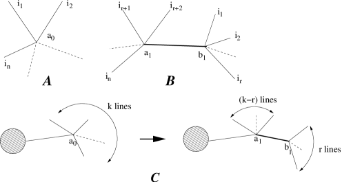
Figure 1: Connected tree level correlators of the collective theory

Consider first the simplest diagram for a $n$-point function, figure A, which is a star graph. The net sign of the diagram is $(-1)^{n+1}\times(-1)^{n}=-1$, where the first factor is from the vertex $a_{0}$ and the second one from the number of lines. Now we proceed to construct all other tree level diagrams from A, by pulling ‘$r$’ lines resulting in figure B, which now has vertices, $a_{1}$ and $b_{1}$ joined by a new line. It is easy to see, that the sign of figure A is not changed by this operation. The net sign of figure B is $(-1)^{(n-r+1)+1}\times(-1)^{(r+1)+1}\times(-1)^{(n+1)}=-1$, where the 3 factors are from $a_{1}$, $b_{1}$ and the number of lines respectively. In figure C we repeat this method for the substar diagrams until we exhaust all possibilities. It is easy to see that the sign stays invariant. Assigning a sign $\alpha$ to the blob, we first find the net sign of the left diagram in figure C. It turns out to be, $\alpha\times(-1)^{(k+1)+1}\times(-1)^{k+1}=-\alpha$. After the “pulling” operation we get $\alpha\times(-1)^{(k-r+2)+1}\times(-1)^{(r+1)+1}\times(-1)^{k+1+1}=-\alpha$. Thus it is proved that in every move the sign is preserved. This proves the relationship (3.35) for all correlation functions.

3.3 $Sp(2N)$ Correlators

Our discussion of the bosonic $O(N)$ collective field theory shows that the $Sp(2N)$ collective field theory in momentum space is a straightforward generalization. In this subsection we discuss the relevant features of the collective theory for the free $Sp(2N)$ model.

The collective Hamiltonian is again exactly the same as in the $O(N)$ theory, given by (3.29) with $\sigma\rightarrow\rho$. Since the connected correlators of the collective fields satisfy

$$\langle\rho({\vec{k}}_{1},{\vec{k}}_{1}^{\prime},t_{1})\rho({\vec{k}}_{2},{\vec{k}}_{2}^{\prime},t_{2})\cdots\rho({\vec{k}}_{n},{\vec{k}}_{n}^{\prime},t_{n})\rangle^{conn}_{Sp(2N)}=-\langle\sigma({\vec{k}}_{1},{\vec{k}}_{1}^{\prime},t_{1})\sigma({\vec{k}}_{2},{\vec{k}}_{2}^{\prime},t_{2})\cdots\sigma({\vec{k}}_{n},{\vec{k}}_{n}^{\prime},t_{n})\rangle^{conn}_{SO(2N)}$$ (3.47)

we now need to choose the negative saddle point,

$$\rho_{0}({\vec{k}},{\vec{k}}^{\prime},t)=-\frac{N}{|{\vec{k}}|}\delta({\vec{k}}-{\vec{k}}^{\prime})$$ (3.48)

The fluctuation Hamiltonian once again has a factor of $(-1)^{n+1}$ for the $n$-point vertex. In particular, the propagator of the collective field is negative of that of the $O(N)$ collective field - the quadratic Hamiltonian has an overall negative sign! This is required - the diagramatic argument for the $Sp(2N)$ oscillator generalizes in a straightforward fashion, ensuring that (3.47) holds.

4 Bulk Dual of the $Sp(2N)$ model

In [6], it was proposed that the collective field theory for the $d$ dimensional free $O(N)$ theory is in fact Vasiliev’s higher spin theory in AdS_d+1. It is easy to see that the collective field has the right collection of fields. Consider for example $d=3$. The field depends on four spatial variables, which may be reorganized as three spatial coordinates one of which is restricted to be positive and an angle. A fourier series in the angle then gives rise to a set of fields $\chi_{\pm n}$ which depend on three spatial variables, with the integer $n$ denoting the conjugate to the angle. Symmetry under interchange of the arguments of the collective field then requires $n$ to be even integers. But this is precisely the content of a theory of massless even spin fields in four space-time dimensions, with $n$ labelling the spin and the two signs corresponding to the two helicities. (Recall that in four space-time dimensions massless fields with any spin have just two helicity states).

The precise relationship between collective fields and higher spin fields in AdS was found in [7] which we now summarize for $d=3$. The correspondence is formulated in the light front quantization. Denote the usual Minkowski coordinates on the space-time on which the $O(N)$ fields live by $t,y,x$ and define light cone coordinates

$$x^{\pm}=\frac{1}{\sqrt{2}}(t\pm y)$$ (4.49)

The conjugate momenta to $x^{+},x^{-}$ are denoted by $p^{-},p^{+}$. Then in light front quantization where $x^{+}$ is treated as time, the Schrodinger picture fields are $\phi^{i}(x^{-},x)$ while the momentum space fields are given by $\phi^{i}(p^{+},p)$. The corresponding collective field is then defined as

$$\sigma(p^{+}_{1},p_{1};p^{+}_{2},p_{2})=\phi^{i}(p^{+}_{1},p_{1})\phi^{i}(p^{+}_{2},p_{2})$$ (4.50)

The fluctuation of this field around the saddle point is denoted by $\Psi(p^{+}_{1},p_{1};p^{+}_{2},p_{2})$. Now define the following bilocal field

$$\Phi(p^{+},p^{x},z,\theta)=\int dp^{z}dp_{1}^{+}dp_{2}^{+}dp_{1}dp_{2}~{}K(p^{+},p^{x},z,\theta;p^{+}_{1},p_{1},p^{+}_{2},p_{2})\Psi(p^{+}_{1},p_{1};p^{+}_{2},p_{2})$$ (4.51)

where the kernel is given by

$$K(p^{+},p^{x},z,\theta;p^{+}_{1},p_{1},p^{+}_{2},p_{2}) = z~{}e^{izp_{z}}~{}\delta(p^{+}_{1}+p^{+}_{2}-p^{+})~{}\delta(p_{1}+p_{2}-p)$$

$$\delta(p_{1}\sqrt{\frac{p_{2}^{+}}{p_{1}^{+}}}-p_{2}\sqrt{\frac{p_{1}^{+}}{p_{2}^{+}}}-p^{z})~{}\delta(2\tan^{-1}\sqrt{\frac{p_{2}^{+}}{p_{1}^{+}}}-\theta)$$

In [7] it was shown that the Fourier transforms of the field $\Phi(p^{+},p^{x},z,\theta)$ with respect to $\theta$ satisfy the same linearized equation of motion as the physical helicity modes of higher spin gauge fields in AdS₄ in light cone gauge. The metric of this AdS₄ is given by the standard Poincare form

$$ds^{2}=\frac{1}{z^{2}}[-2dx^{+}dx^{-}+dx^{2}+dz^{2}]=\frac{1}{z^{2}}[-dt^{2}+dy^{2}+dx^{2}+dz^{2}]$$ (4.52)

The momenta $p^{+},p$ are conjugate to $x^{-},x$. The additional dimension generated from the large-N degrees of freedom is $z$, which is canonically conjugate to $p^{z}$ and is given in terms of the phase space coordinate of the bi-locals by

$$z=\frac{(x_{1}-x_{2})\sqrt{p^{+}_{1}p^{+}_{2}}}{p^{+}_{1}+p^{+}_{2}}$$ (4.53)

In particular, the linearized equation for the spin zero field, $\varphi(x^{-},x,z)$, follows from the quadratic action

$$S=\frac{1}{2}\int dx^{+}dx^{-}dzdx~{}\left[\frac{1}{z^{2}}\left(-2\partial_{+}\varphi\partial_{-}\varphi-(\partial_{x}\varphi)^{2}-(\partial_{z}\varphi)^{2}\right)+\frac{2}{z^{4}}\varphi^{2}\right]$$ (4.54)

which is of course the action of a conformally coupled scalar in the AdS₄ with coordinates given by (4.53). The actions for the spin-$2s$ fields can be similarly written down. Even though these actions are derived using light cone coordinates, they can be covariantized easily since these are free actions. In terms of the coordinates $t,y,x,z$ the scalar action is given by

$$S=\frac{1}{2}\int dtdzdxdy~{}\left[\frac{1}{z^{2}}\left((\partial_{t}\varphi)^{2}-(\partial_{y}\varphi)^{2}-(\partial_{x}\varphi)^{2}-(\partial_{z}\varphi)^{2}\right)+\frac{2}{z^{4}}\varphi^{2}\right]$$ (4.55)

Let us now turn to the $Sp(2N)$ collective theory. One can define once again the fields as in (4.51) and (4). The coordinates $(x^{+},x^{-},x,z)$ will continue to transform appropriately under AdS isometries. However, we saw earlier that the quadratic part of the Hamiltonian, and therefore the quadratic part of the action will have an overall negative sign.

A negative kinetic term signifies a pathology. Indeed we derived this theory with the Lorentzian signature $Sp(2N)$ model, which has negative norm states. The negative kinetic term of the collective theory is possibly intimately related to this lack of unitarity.

However, the form of the action (4.55) cries out for a analytic continuation

$$z=i\tau~{}~{},~{}~{}~{}~{}~{}~{}t=-iw$$ (4.56)

Under this continuation the action, $S$ becomes

$$S^{\prime}=\frac{1}{2}\int d\tau dwdxdy~{}\left[\frac{1}{\tau^{2}}\left((\partial_{\tau}\varphi)^{2}-(\partial_{y}\varphi)^{2}-(\partial_{x}\varphi)^{2}-(\partial_{w}\varphi)^{2}\right)-\frac{2}{\tau^{4}}\varphi^{2}\right]$$ (4.57)

The sign of the mass term has not changed in this analytic continuation, and this action has become the action of a conformally coupled scalar field in de Sitter space with the metric

$$ds^{2}=\frac{1}{\tau^{2}}[-d\tau^{2}+dx^{2}+dy^{2}+dw^{2}]$$ (4.58)

This mechanism works for all even higher spin fields at the quadratic level.

To summarize, the collective field theory of the three dimensional Lorentzian $Sp(2N)$ model can be written as a theory of massless even spin fields in AdS₄, but with negative kinetic terms. Under a double analytic continuation this becomes the action in dS₄ with positive kinetic terms. This is consistent with the conjecture of [16] that the euclidean $Sp(N)$ model is dual to Vasiliev theory in dS₄. It is interesting to note that the way an emergent holographic direction is similar to the way the Liouville mode has to be interpeted as a time dimension in worldsheet supercritical string theory [17]. In this latter case, the sign of the kinetic term for the Liouville mode is negative for $d>d_{cr}$.

Even for the $O(N)$ model, the collective field is an represents seemingly an overcomplete description, since for a finite number of points in space $K$, one replaces at most $NK$ variables by $K^{2}$ variables, which is much larger in the thermodynamic and continuum limit. However, in the perturbative $1/N$ expansion this is not an issue and the collective theory is known to reproduce the standard results of the $O(N)$ model. The issue becomes of significance at finite $N$ level.The relevance of incorporating for such features has been noted in [18, 31].

For the fermionic $Sp(2N)$ model, there appears potentially an even more important redundancy related to the Grassmannian origin of the construction. Consequently the fields are to obey nontrivial constraint relationships and the Hilbert space is subject to a cutoff of highly excited states. This ‘exclusion principle’ was noted already in the AdS correspondence involving $S_{N}$ orbifolds[32, 33, 34].

In an expansion around $N=\infty$ most effects of this are invisible and our discussion shows that this can be regarded as a theory of higher spin fields in dS is insensitive to these effects. However, as we saw above, the Grassmann origin was already of importance in choosing the correct saddle point and the correct quanization of the quadratic hamiltonian. In the next section we will address the question of finite $N$ and the Hilbert space of the bi-local theory. In the framework of geometric (pseudospin) representation we will give evidence that the bi-local theory is non-perturbatively satisfactory at the finite $N$ level.

5 Geometric Representation and The Hilbert Space

The bi-local collective field representation is seen to give a bulk description dS space and the Higher Spin fields. It provides an interacting theory with vertices governed by $G=1/N$ as the coupling constant. We would now to show that the collective theory has an equivalent geometric (Pseudo) Spin variable description appropriate for nonperturbative considerations. The essence of this (geometric) description is in reinterpreting the bi-local collective fields (and their canonical conjugates) as matrix variables (of infinite dimensionality) endowed with a Kahler structure.This geometric description will provide a tractable framework for quantization and non-perturbative definition of the bi-local and HS de Sitter theory. It will be seen capable to incorporate non-perturbative features related to the Grassmannian origin of bi-local fields and its Hilbert space. Pseudo-spin collective variables represent all $Sp(2N)$ invariant variables of the theory (both commuting and non-commuting). These close a compact algebra and at large $N$ are constrained by the corresponding Casimir operator. One therefore has an algebraic pseudo-spin system whose nonlinearity is governed by the coupling constant $G=1/N$. As such they have been employed earlier for developing a large $N$ expansion [35] and as a model for quantization [36]. This version of the theory is in its perturbative ($1/N$) expansion identical to the bi-local collective representation. It therefore has the same map to and correspondence with Higher Spin dS₄ at perturbative level. We will see however that the geometric representation becomes of use for defining (and evaluating) the Hilbert space and its quantization.

To describe the pseudo-spin description of the $Sp(2N)$ theory we will follow the quantization procedure of [37]. In this approach one starts from the action:

$$S=\int d^{d}x\;dt(\partial^{\mu}\eta^{i}_{1}\partial_{\mu}\eta^{i}_{2})$$ (5.59)

and deduces the canonical anti-commutation relations

$$\{\eta^{i}_{1}(x,t)\partial_{t}\eta^{j}_{2}(x^{\prime},t)\}=-\{\eta^{i}_{2}(x,t)\partial_{t}\eta^{j}_{1}(x^{\prime},t)\}=i\delta^{d}(x-x^{\prime})\delta^{ij}$$ (5.60)

The quantization based on the mode expansion

$$\eta^{i}_{1}(x) = \int\frac{d^{d}k}{(2\pi)^{d/2}\sqrt{2\omega_{k}}}(a_{k+}^{i\dagger}e^{-ikx}+a^{i}_{k-}e^{ikx})$$ (5.61)

$$\eta^{i}_{2}(x) = \int\frac{d^{d}k}{(2\pi)^{d/2}\sqrt{2\omega_{k}}}(-a_{k-}^{i\dagger}e^{-ikx}+a^{i}_{k+}e^{ikx})$$ (5.62)

with

$$\{a^{i}_{k-},a_{k^{\prime}-}^{j\dagger}\}=\{a^{i}_{k+},a_{k^{\prime}+}^{j\dagger}\}=\delta^{d}(k-k^{\prime})\delta^{ij}$$ (5.63)

Note that in this approach the operators $\eta^{i}_{a}$ are not hermitian, but pseudo-hermitian in the sense of [38].

Pseudo-spin bi-local variables will be introduced based on $Sp(2N)$ invariance, we have the vectors:

$$\eta = (\eta_{1}^{1},\eta_{2}^{1},\eta_{1}^{2},\eta_{2}^{2},\cdots,\eta_{1}^{N},\eta_{2}^{N})$$ (5.64)

$$a(k) = (a^{1}_{k-},a_{k+}^{1},a^{2}_{k-},a_{k+}^{2},\cdots,a^{N}_{k-},a_{k+}^{N})$$ (5.65)

$$\tilde{a}(k) = (a_{k+}^{1\dagger},-a^{1\dagger}_{k-},a_{k+}^{2\dagger},-a^{2\dagger}_{k-},\cdots,a_{k\dagger}^{N+},-a^{N\dagger}_{k-})$$ (5.66)

and the notation:

$$\eta(x)=\int\frac{d^{d}k}{(2\pi)^{d/2}\sqrt{2\omega_{k}}}(\tilde{a}(k)e^{-ikx}+a(k)e^{ikx})$$ (5.67)

so that a complete set of $Sp(2N)$ invariant operators now follows:

$$S(p_{1},p_{2}) = \frac{-i}{2\sqrt{N}}a^{T}(p_{1})\epsilon_{N}a(p_{2})=\frac{i}{2\sqrt{N}}\sum_{i=1}^{N}(a_{p_{1}+}^{i}a_{p_{2}-}^{i}+a_{p_{2}+}^{i}a_{p_{1}-}^{i})$$ (5.68)

$$S^{\dagger}(p_{1},p_{2}) = \frac{-i}{2\sqrt{N}}\tilde{a}^{T}(p_{1})\epsilon_{N}\tilde{a}(p_{2})=\frac{i}{2\sqrt{N}}\sum_{i=1}^{N}(a_{p_{1}+}^{i\dagger}a_{p_{2}-}^{i\dagger}+a_{p_{2}+}^{i\dagger}a_{p_{1}-}^{i\dagger})$$ (5.69)

$$B(p_{1},p_{2}) = \tilde{a}^{T}(p_{1})\epsilon_{N}a(p_{2})=\sum_{i=1}^{N}a_{p_{1}+}^{i\dagger}a_{p_{2}+}^{i}+a_{p_{1}-}^{i\dagger}a_{p_{2}-}^{i}$$ (5.70)

and $\epsilon_{N}=\epsilon\otimes\mathbb{I}_{N}$, $\epsilon=\left(\begin{array}[]{cc}0&1\\ -1&0\end{array}\right)$

These invariant operators close an invariant algebra. The commutation relations are found to equal:

$$\big{[}S(\vec{p}_{1},\vec{p}_{2}),S^{\dagger}(\vec{p}_{3},\vec{p}_{4})\big{]}= {1\over 2}\left(\delta_{\vec{p}_{2},\vec{p}_{3}}\delta_{\vec{p}_{4},\vec{p}_{1}}+\delta_{\vec{p}_{2},\vec{p}_{4}}\delta_{\vec{p}_{3},\vec{p}_{1}}\right)-{1\over{4N}}\left[\delta_{\vec{p}_{2},\vec{p}_{3}}B(\vec{p}_{4},\vec{p}_{1})+\delta_{\vec{p}_{2},\vec{p}_{4}}B(\vec{p}_{3},\vec{p}_{1})\right.$$ (5.72)

$$+\left.\delta_{\vec{p}_{1},\vec{p}_{3}}B(\vec{p}_{4},\vec{p}_{2})+\delta_{\vec{p}_{1},\vec{p}_{4}}B(\vec{p}_{3},\vec{p}_{2})\right]$$

$$\big{[}B(\vec{p}_{1},\vec{p}_{2}),S^{\dagger}(\vec{p}_{3},\vec{p}_{4})\big{]}= \delta_{\vec{p}_{2},\vec{p}_{3}}S^{\dagger}(\vec{p}_{1},\vec{p}_{4})+\delta_{\vec{p}_{2},\vec{p}_{4}}S^{\dagger}(\vec{p}_{1},\vec{p}_{3})$$ (5.73)

$$\big{[}B(\vec{p}_{1},\vec{p}_{2}),S(\vec{p}_{3},\vec{p}_{4})\big{]}= -\delta_{\vec{p}_{1},\vec{p}_{3}}S(\vec{p}_{2},\vec{p}_{4})-\delta_{\vec{p}_{1},\vec{p}_{4}}S(\vec{p}_{2},\vec{p}_{3})$$ (5.74)

The singlet sector of the original $Sp(2N)$ theory is characterized by a further constraint. This constraint is is associated with the Casimir operator of of the algebra and can be shown to take the form:

$$\frac{4}{N}S^{\dagger}\star S+(1-\frac{1}{N}B)\star(1-\frac{1}{N}B)=\text{$\mathbb{I}$}$$ (5.75)

Here we have used the matrix star product notation: $\star$ product as: with $A\star B=\int d\vec{p}_{2}A(\vec{p}_{1}\vec{p}_{2})B(\vec{p}_{2}\vec{p}_{3})$.

The form of the Casimir, which commutes with the above pseudo-spin fields points to the compact nature of the bi-local pseudo-spin algebra associated with the $Sp(2N)$ theory. This will have major consequences which we will highlight later.

Indeed it is interesting to compare the algebra with the bosonic case, where we have:

$$S(p_{1},p_{2}) = \frac{1}{2\sqrt{N}}\sum_{i=1}^{2N}a_{i}(p_{1})a_{i}(p_{2})$$ (5.76)

$$S^{\dagger}(p_{1},p_{2}) = \frac{1}{2\sqrt{N}}\sum_{i=1}^{2N}a_{i}^{\dagger}(p_{1})a_{i}^{\dagger}(p_{2})$$ (5.77)

$$B(p_{1},p_{2}) = \sum_{i=1}^{2N}a_{i}^{\dagger}(p_{1})a_{i}(p_{2})$$ (5.78)

with the commutation relations:

$$\big{[}S(\vec{p}_{1},\vec{p}_{2}),S^{\dagger}(\vec{p}_{3},\vec{p}_{4})\big{]}= {1\over 2}\left(\delta_{\vec{p}_{2},\vec{p}_{3}}\delta_{\vec{p}_{4},\vec{p}_{1}}+\delta_{\vec{p}_{2},\vec{p}_{4}}\delta_{\vec{p}_{3},\vec{p}_{1}}\right)+{1\over{4N}}\left[\delta_{\vec{p}_{2},\vec{p}_{3}}B(\vec{p}_{4},\vec{p}_{1})+\delta_{\vec{p}_{2},\vec{p}_{4}}B(\vec{p}_{3},\vec{p}_{1})\right.$$ (5.80)

$$+\left.\delta_{\vec{p}_{1},\vec{p}_{3}}B(\vec{p}_{4},\vec{p}_{2})+\delta_{\vec{p}_{1},\vec{p}_{4}}B(\vec{p}_{3},\vec{p}_{2})\right]$$

$$\big{[}B(\vec{p}_{1},\vec{p}_{2}),S^{\dagger}(\vec{p}_{3},\vec{p}_{4})\big{]}= \delta_{\vec{p}_{2},\vec{p}_{3}}S^{\dagger}(\vec{p}_{1},\vec{p}_{4})+\delta_{\vec{p}_{2},\vec{p}_{4}}S^{\dagger}(\vec{p}_{1},\vec{p}_{3})$$ (5.81)

$$\big{[}B(\vec{p}_{1},\vec{p}_{2}),S(\vec{p}_{3},\vec{p}_{4})\big{]}= -\delta_{\vec{p}_{1},\vec{p}_{3}}S(\vec{p}_{2},\vec{p}_{4})-\delta_{\vec{p}_{1},\vec{p}_{4}}S(\vec{p}_{2},\vec{p}_{3})$$ (5.82)

In this case the Casimir constraint is found to equal:

$$-\frac{4}{N}S^{\dagger}\star S+(1+\frac{1}{N}B)\star(1+\frac{1}{N}B)=\text{$\mathbb{I}$}$$ (5.83)

featuring the non-compact nature of the bosonic problem.

We can see therefore that the singlet sectors of the fermionic $Sp(2N)$ theory and the bosonic $O(2N)$ theory can be described in analogous a bi-local pseudo-spin algebraic formulations with a quadratic Casimir taking the form:

$$4\gamma S^{\dagger}\star S+(1-\gamma B)\star(1-\gamma B)=\text{$\mathbb{I}$}$$ (5.84)

the difference being that with $\gamma=\frac{1}{N}(-\frac{1}{N})$ for the fermionic (bosonic) case respectively. This signifies the compact versus the non-compact nature of the algebra, but also exhibits the relationship obtained through the $N\leftrightarrow-N$ switch that was central in the argument for de Sitter correspondence in [16].

From this algebraic bi-local formulation one can easily see the the Collective field representation(s) that we have discussed in sections 2 and 3. Very simply, the Casimir constraints can be solved, and the algebra implemented in terms of a canonical pair of bi-local fields:

$$S(p_{1}p_{2}) = \frac{\sqrt{-\gamma}}{2}\int dy_{1}dy_{2}e^{-i(p_{1}y_{2}+p_{2}y_{2})}\{-\frac{2}{\kappa_{p_{1}}\kappa_{p_{2}}}\Pi\star\Psi\star\Pi(y_{1}y_{2})-\frac{1}{2\gamma^{2}\kappa_{p_{1}}\kappa_{p_{2}}}\frac{1}{\Psi}(y_{1}y_{2})$$ (5.86)

$$+\frac{\kappa_{p_{1}}\kappa_{p_{2}}}{2}\Psi(y_{1}y_{2})-i\frac{\kappa_{p_{1}}}{\kappa_{p_{2}}}\Psi\star\Pi(y_{1}y_{2})-i\frac{\kappa_{p_{2}}}{\kappa_{p_{1}}}\Pi\star\Psi(y_{1}y_{2})\}$$

$$S^{\dagger}(p_{1}p_{2}) = \frac{\sqrt{-\gamma}}{2}\int dy_{1}dy_{2}e^{-i(p_{1}y_{2}+p_{2}y_{2})}\{-\frac{2}{\kappa_{p_{1}}\kappa_{p_{2}}}\Pi\star\Psi\star\Pi(y_{1}y_{2})-\frac{1}{2\gamma^{2}\kappa_{p_{1}}\kappa_{p_{2}}}\frac{1}{\Psi}(y_{1}y_{2})$$ (5.88)

$$+\frac{\kappa_{p_{1}}\kappa_{p_{2}}}{2}\Psi(y_{1}y_{2})+i\frac{\kappa_{p_{1}}}{\kappa_{p_{2}}}\Psi\star\Pi(y_{1}y_{2})+i\frac{\kappa_{p_{2}}}{\kappa_{p_{1}}}\Pi\star\Psi(y_{1}y_{2})\}$$

$$B(p_{1}p_{2}) = \frac{1}{\gamma}+\int dy_{1}dy_{2}e^{-i(p_{1}y_{2}+p_{2}y_{2})}\{\frac{2}{\kappa_{p_{1}}\kappa_{p_{2}}}\Pi\star\Psi\star\Pi(y_{1}y_{2})+\frac{1}{2\gamma^{2}\kappa_{p_{1}}\kappa_{p_{2}}}\frac{1}{\Psi}(y_{1}y_{2})$$ (5.90)

$$+\frac{\kappa_{p_{1}}\kappa_{p_{2}}}{2}\Psi(y_{1}y_{2})-i\frac{\kappa_{p_{1}}}{\kappa_{p_{2}}}\Psi\star\Pi(y_{1}y_{2})+i\frac{\kappa_{p_{2}}}{\kappa_{p_{1}}}\Pi\star\Psi(y_{1}y_{2})\}$$

where $\kappa_{p}=\sqrt{\omega_{p}}$.

Recalling that the Hamiltonian is given in terms of $B$ we now see that its bi-local form is the same in the fermionic and the bosonic case. This explains the feature that we have established by direct construction in Sec. 2,3. While the bi-local field representation of $B$ is the same in the fermionic and bosonic cases, the difference is seen in the representations of operators $S$ and $S^{\dagger}$. These operators create singlet states in the Hilbert space and the difference contained in the sign of gamma implies the opposite shifts for the background fields that we have identified in Sec. 2,3. The algebraic pseudo spin reformulation is therefore seen to account for all the perturbative ($1/N$) features of the the bi-local theory that we have identified in Sec. 2,3. However, in addition and we would like to emphasize that, the algebraic formulation provides a proper framework for defining the bi-local Hilbert space.

5.1 Quantization and the Hilbert Space

The bi-local pseudo-spin algebra has several equivalent representations that turn out to be useful. Beside that collective representation that we have explained above, one has the simple oscillator representation:

$$S(p_{1},p_{2}) = \alpha\star(1-\frac{1}{N}\alpha^{\dagger}\star\alpha)^{\frac{1}{2}}(p_{1},p_{2})$$ (5.91)

$$S^{\dagger}(p_{1},p_{2}) = (1-\frac{1}{N}\alpha^{\dagger}\star\alpha)^{\frac{1}{2}}\star\alpha^{\dagger}(p_{1},p_{2})$$ (5.92)

$$B(p_{1},p_{2}) = 2\;\alpha^{\dagger}\star\alpha(p_{1},p_{2})$$ (5.93)

with standard canonical canonical commutators (or Poisson brackets).

A more relevant geometric representation is obtained through a change:

$$\alpha = Z(1+\frac{1}{N}\bar{Z}Z)^{-\frac{1}{2}}$$ (5.94)

$$\alpha^{\dagger} = (1+\frac{1}{N}\bar{Z}Z)^{-\frac{1}{2}}\bar{Z}$$ (5.95)

The pseudo-spins in the $Z$ representation are given by:

$$S(p_{1},p_{2}) = Z\star(1+\frac{1}{N}\bar{Z}\star Z)^{-1}(p_{1},p_{2})$$ (5.96)

$$S^{\dagger}(p_{1},p_{2}) = (1+\frac{1}{N}\bar{Z}\star Z)^{-1}\star\bar{Z}(p_{1},p_{2})$$ (5.97)

$$B(p_{1},p_{2}) = 2\;Z\star(1+\frac{1}{N}\bar{Z}\star Z)^{-1}\star\bar{Z}(p_{1},p_{2})$$ (5.98)

It’s easy to see that this satisfy the Casimir constraint: $\frac{4}{N}S^{\dagger}\star S+(1-\frac{1}{N}B)^{2}=1$

One can write the Lagrangian in this $Z$ representation as:

$$\text{$\mathcal{L}$}=i\int dt\;\text{tr}[Z(1+\frac{1}{N}\bar{Z}Z)^{-1}\dot{\bar{Z}}-\dot{Z}(1+\frac{1}{N}\bar{Z}Z)^{-1}\bar{Z}]-\text{$\mathcal{H}$}$$ (5.99)

For regularization purposes, it is useful to consider putting $\vec{x}$ in a box and limiting the momenta by a cutoff $\Lambda$: this makes the bi-local fields into finite dimensional matrices (which we will take to be a size $K$). For $Sp(2N)$ one deals with a $K\times K$ dimensional complex matrix $Z$ and we have obtained in the above a compact symmetric (Kahler) space :

$$ds^{2}=\text{tr}[dZ(1-\bar{Z}Z)^{-1}d\bar{Z}(1-Z\bar{Z})^{-1}]$$ (5.100)

According to the classification of [39], this would correspond to manifold $M_{I}(K,K)$. We note that the standard fermionic problem which was considered in detail in [36] corresponds to manifold $M_{{III}}(K,K)$ of complex antisymmetric matrices.

Quantization on Kahler manifolds in general has been formulated in detail by Berezin [36]. We also note that the usefullnes of Kahler quantization for discretizing de Sitter space was pointed out by A. Volovich in a quantum mechanical scenario[22]. In the present Quantization we are dealing with a field theory with infinitely many degrees of freedom and infinite Khaler matrix variables. We will now summarize some of the results of quantization which are directly relevant to the $Sp(2N)$ bi-local collective fields theory. Commutation relations of this system follow from the Poisson Brackets associated with the Lagrangian $\mathcal{L}(\bar{Z},Z)$. States in the Hilbert space are represented by (holomorphic) functions (functionals) of the bi-locals $Z(k,l)$. A Kahler scalar product defining the bi-local Hilbert space reads:

$$(F_{1},F_{2})=C(N,K)\int d\mu(\bar{Z},Z)F_{1}(Z)F_{2}(\bar{Z})\det[1+\bar{Z}Z]^{-N}$$ (5.101)

with the (Kahler) integration measure:

$$d\mu=\det[1+\bar{Z}Z]^{-2K}d\bar{Z}dZ$$ (5.102)

The normalization constant is found from requiring $(F_{1},F_{1})=1$ for $F=1$. Let:

$$a(N,K)=\frac{1}{C(N,K)}=\int d\mu(\bar{Z},Z)\det[1+\bar{Z}Z]^{-N}$$ (5.103)

This leads to the matrix integral (complex Penner Model)

$$a(N,K)=\frac{1}{C(N,K)}=\int\prod_{k,l=1}^{K}d\bar{Z}(k,l)dZ(k,l)\det[1+\bar{Z}Z]^{-2K-N}$$ (5.104)

which determines $C(N,K)$.

The following results on quantization of this type of Kahler system are of note: First, the parameter $N$: much like for ordinary spin, one can show that $N$ (and therefore $G$ in Higher Spin Theory) can only take integer values, i.e. $N=0,1,2,3,\cdots$. Next, one has question about the total number of states in the above Hilbert space. Naively, bi-local theory would seem to grossly overcount the number of states of the original fermionic theory. Originally one essentially had $2NK$ fermionic degrees of freedom with a finite Hilbert space. The bi-local description is based on (complex) bosonic variables of dimensions $K^{2}$ and the corresponding Hilbert space would appear to be much larger. But due to the compact nature of the phase space, the number of states much smaller.

We will now evaluate this number (at finite $N$ and $K$) for the present case of $Sp(2N)$ (in [36] ordinary fermions were studied) and show that the exact dimension of the bi-local Hilbert space in geometric (Kahler) quantization agrees with the dimension of the singlet Hilbert space of the $Sp(2N)$ fermionic theory.

The dimension of quantized Hilbert space is found as follows: Considering the operator $\hat{O}=I$ one has that:

$$\text{Tr}(I)=C(N,K)\int\prod_{k,l=1}^{K}d\bar{Z}(k,l)dZ(k,l)\det[1+\bar{Z}Z]^{-2K}$$ (5.105)

Consequently the dimension of the bi-local Hilbert space is given by:

$$\text{Dim $\mathcal{H}$}_{B}=\frac{C(N,K)}{C(0,K)}=\frac{a(0,K)}{a(N,K)}$$ (5.106)

The evaluation of the matrix (Penner) integral therefore also determines the dimension of the bi-local Hilbert space. Since this evaluation is a little bit involved, we present it in the following. Evaluation of matrix integrals (for real matrices) is given in [40] the extension to the complex case was considered in[41].

We will use results of [39], whereby every (complex) matrix can be reduced through (symmetry) transformations to a diagonal form:

$$Z(k,l)\rightarrow\begin{bmatrix}\omega_{1}&&&&\\ &\omega_{2}&&\text{\huge{0}}&\\ &&\omega_{3}&&\\ &\text{\huge{0}}&&\ddots&\\ &&&&\omega_{K}\end{bmatrix}$$ (5.107)

and the matrix integration measure becomes:

$$[d\bar{Z}dZ]=|\Delta(\omega)|^{2}\prod_{l=1}^{K}d\omega_{l}d\Omega$$ (5.108)

where $d\Omega$ denotes “angular” parts of the integration and $\Delta(x_{1},\cdots,x_{K})=\prod_{k<l}(x_{k}-x_{l})$ is a Vandermonde determinant, with $x_{i}=\omega_{i}^{2}$. Consequently the matrix integral for $a(N,K)$ (and $C(N,K)$) becomes:

$$a(N,K)=\frac{\text{Vol}\;\;\Omega}{K!}\int\Delta(x_{1},\cdots,x_{K})^{2}\prod_{l}(1+\omega_{l}^{2})^{-2K-N}\prod_{l}d\omega_{l}$$ (5.109)

changing variables: $x_{i}=-\frac{y_{i}}{1-y_{i}}$, we get:

$$a(N,K)=\frac{\text{Vol}\;\;\Omega}{2^{K}K!}\int_{0}^{\Lambda}\prod_{i}^{K}dy_{i}\Delta(y_{1},\cdots,y_{K})^{2}\prod_{i}(1-y_{i})^{N}$$ (5.110)

This integral can be evaluated exactly. It belongs to a class of integrals evaluated by Selberg in 1944 [42]:

$$I(\alpha,\beta,\gamma,n) = \int_{0}^{1}dx_{1}\cdots\int_{0}^{1}dx_{n}|\Delta(x)|^{2\gamma}\prod_{j=1}^{n}x_{j}^{\alpha-1}(1-x_{j})^{\beta-1}$$ (5.111)

$$= \prod_{j=0}^{n-1}\frac{\Gamma(1+\gamma+j\gamma)\Gamma(\alpha+j\gamma)\Gamma(\beta+j\gamma)}{\Gamma(1+\gamma)\Gamma(\alpha+\beta+(n+j-1)\gamma)}$$ (5.112)

we have the case with $\alpha=1,\;\;\beta=N+1,\;\;\gamma=1,\;\;n=K$ and

$$I(1,N+1,1,K) = \prod_{j=0}^{K-1}\frac{\Gamma(2+j)\Gamma(1+j)\Gamma(N+1+j)}{\Gamma(2)\Gamma(N+K+j+1)}$$ (5.113)

We therefore obtain the following formula for the number of states in our Bi-local $Sp(2N)$ Hilbert space:

$$\text{Dim $\mathcal{H}$}_{B}=\prod_{j=0}^{K-1}\frac{\Gamma(j+1)\Gamma(N+K+j+1)}{\Gamma(K+j+1)\Gamma(N+j+1)}$$ (5.114)

We have compared this number with explicit enumeration of $Sp(2N)$ invariant states in the fermionic Hilbert space (for low values of $N$ and $K$) and found complete agreement. It is probably not that difficult to prove agreement for all $N,K$. This settles however the potential problem of overcompletness of the bi-local representation. Since the $Sp(2N)$ counting uses the fermionic nature of creation operators and features exclusion when occupation numbers grow above certain limit it is seen that bi-local geometric quantization elegantly incorporates these effects. The compact nature of the associated infinite dimensional Kahler manifold secures the correct dimensionality of the the singlet Hilbert space. By using Stirling’s approximation for the number of states in the bi-local Hilbert space (5.114), we see the dimension growing linearly in $N$ (with $K\gg N$):

$$\ln(\text{Dim $\mathcal{H}$}_{B})\sim 2NK\;\ln 2\qquad\text{at the leading order}$$ (5.115)

This is a clear demonstration of the presence of an $N$-dependent cutoff in agreement with the fermionic nature of the original $Sp(2N)$ Hilbert space. So in the nonlinear bi-local theory with $G=1/N$ as coupling constant, we have the desired effect that the Hilbert space is cutoff through $1/G$ effects. Consequently we conclude that the geometric bi-local representation with infinite dimensional matrices $Z(k,l)$ provides a complete framework for quantization of the bi-local theory and of de Sitter HS Gravity.

6 Comments

We have motivated the use of double analytic continuation and hence the connection between the $Sp(2N)$ model and de Sitter higher field theory for the quadratic action for the collective field. To establish this connection one of course needs to establish this for the interaction terms. This is of course highly nontrivial, and in fact the connection between the collective theory for the $O(N)$ model and the AdS higher spin theory is only beginning to be understood. We believe that once this is understood well enough one can address the question for the $Sp(2N)$-dS connection.

In this paper we have dealt mostly with the free $Sp(2N)$ vector model. As the parallel $O(N)$/AdS case this theory is characterized with an infinite sequence of conserved higher spin currents and associated conserved charges. The question regarding the implementation of the Coleman-Mandula theorem then arises, this question was discussed recently in [43, 44, 45]. One can expected that identical conclusions hold for the present $Sp(2N)$ case. The bi-local collective field theory technqiue is trivially extendible to the linear sigma model based on $Sp(2N)$, as commented in section (4.2). Of particular interest is the IR behavior of the theory which presumably takes the theory from the Gaussian fixed point to a nontrivial fixed point.

It is well known that dS/CFT correspondence is quite different from AdS/CFT correspondence, particularly in the interpretation of bulk correlation functions [15, 46]. We have not addressed these issues in this paper. Recently it has been proposed that the $Sp(2N)$/dS connection can be used to understand subtle points about dS/CFT [18]. We hope that an explicit construction as described in this paper will be valuable for a deeper understanding of these issues.

The bi-local formulation that we have presented was cast in a geometric, pseudo-spin framework. We have suggested that this representation offers the best framework for quantization of the bi-local theory and consequently the Hilbert space in dS/CFT. We have demonstrated through counting of the size of the Hilbert space that it incorporates finite $N$ effects through a cutoff which depends on the coupling constant of the theory: $G=1/N$. Most importantly it incorporates the finite $N$ exclusion principle and provides an explanation on the quantization of $G=1/N$ from the bulk point of view. These features are obviously of definite relevance for understanding quantization of Gravity in de Sitter space-time. Nevertheless the question of understanding de Sitter Entropy from this 3 dimensional CFT remains an interesting and challenging problem.

It would be interesting to consider the analogues of $Sp(2N)$/dS correspondence in the CFT₂/Chern-Simons version[50, 48, 49], as well as to three dimensional conformal theories which have a line of fixed points, as in [51]. Finally higher spin theories arise as limits of string theory in several contexts, e.g. [52] and [51]. It would be interesting to see if these models can be modified to realize a dS/CFT correspondence in string theory.

7 Acknowledgements

The work of D.D. and S.R.D. is partially supported by National Science Foundation grants PHY-0970069 and PHY-0855614. The work of A.J. and Q.Y. is supported by the Department of Energy under contract DE-FG-02-91ER40688. We would like to thank Matthew Dodelson, Misha Eides, Igor Klebanov, Gautam Mandal, Shinji Mukhoyama, Marcus Spradlin, Alfred Shapere and Anastasia Volovich for discussions and Luis Alvarez-Gaume for a comment. S.R.D. thanks PCTS at Princeton University, Theory Group at CERN and University of Barcelona for hospitality during the final stages of the preparation of this manuscript.

References

- [1] I. R. Klebanov and A. M. Polyakov, Phys. Lett. B 550, 213 (2002) [hep-th/0210114].
- [2] For a recent review and a more complete list of original references , see M. A. Vasiliev, arXiv:1203.5554 [hep-th].
- [3] S. Giombi and X. Yin, JHEP 1009, 115 (2010) [arXiv:0912.3462 [hep-th]].
- [4] E. Sezgin and P. Sundell, JHEP 0507, 044 (2005) [hep-th/0305040].
- [5] A. Jevicki and B. Sakita, Nucl. Phys. B 165, 511 (1980).
- [6] S. R. Das and A. Jevicki, “Large-N collective fields and holography,” Phys. Rev. D 68, 044011 (2003) [arXiv:hep-th/0304093].
- [7] R. d. M. Koch, A. Jevicki, K. Jin and J. P. Rodrigues, Phys. Rev. D 83, 025006 (2011) [arXiv:1008.0633 [hep-th]].
- [8] A. Jevicki, K. Jin and Q. Ye, arXiv:1112.2656 [hep-th].
- [9] A. Jevicki, K. Jin and Q. Ye, J. Phys. A A 44, 465402 (2011) [arXiv:1106.3983 [hep-th]].
- [10] M. R. Douglas, L. Mazzucato and S. S. Razamat, Phys. Rev. D 83, 071701 (2011) [arXiv:1011.4926 [hep-th]].
- [11] S. R. Das and A. Jevicki, Mod. Phys. Lett. A 5, 1639 (1990).
- [12] T. Eguchi and H. Kawai, Phys. Rev. Lett. 48, 1063 (1982).
- [13] T. Banks, W. Fischler, S. H. Shenker and L. Susskind, Phys. Rev. D 55, 5112 (1997) [hep-th/9610043].
- [14] N. Ishibashi, H. Kawai, Y. Kitazawa and A. Tsuchiya, Nucl. Phys. B 498, 467 (1997) [hep-th/9612115].
- [15] A. Strominger, JHEP 0110, 034 (2001) [hep-th/0106113]; A. Strominger, JHEP 0111, 049 (2001) [hep-th/0110087];
- [16] D. Anninos, T. Hartman and A. Strominger, arXiv:1108.5735 [hep-th].
- [17] S. R. Das, S. Naik and S. R. Wadia, Mod. Phys. Lett. A 4, 1033 (1989).
- [18] G. S. Ng and A. Strominger, arXiv:1204.1057 [hep-th].
- [19] E. Witten, hep-th/0106109;
- [20] V. Balasubramanian, P. Horava and D. Minic, JHEP 0105, 043 (2001) [hep-th/0103171].
- [21] T. Banks, astro-ph/0305037.
- [22] A. Volovich, hep-th/0101176.
- [23] M. K. Parikh and E. P. Verlinde, JHEP 0501, 054 (2005) [hep-th/0410227].
- [24] D. A. Lowe, Phys. Rev. D 70, 104002 (2004) [hep-th/0407188].
- [25] L. Dyson, J. Lindesay and L. Susskind, JHEP 0208, 045 (2002) [hep-th/0202163]; N. Goheer, M. Kleban and L. Susskind, JHEP 0307, 056 (2003) [hep-th/0212209].
- [26] M. Henneaux and C. Teitelboim, Annals Phys. 143, 127 (1982); M. Henneaux and C. Teitelboim, Princeton, USA: Univ. Pr. (1992) 520 p
- [27] R. Finkelstein and M. Villasante, Phys. Rev. D 33, 1666 (1986).
- [28] R. de Mello Koch and J. P. Rodrigues, Phys. Rev. D 54, 7794 (1996) [hep-th/9605079].
- [29] R. Jackiw and A. Strominger, Phys. Lett. B 99, 133 (1981).
- [30] H. Shimodaira, Nucl. Phys. 17,486 (1960).
- [31] S. H. Shenker and X. Yin, arXiv:1109.3519 [hep-th].
- [32] J. M. Maldacena and A. Strominger, JHEP 9812, 005 (1998) [hep-th/9804085].
- [33] A. Jevicki and S. Ramgoolam, JHEP 9904, 032 (1999) [hep-th/9902059].
- [34] A. Jevicki, M. Mihailescu and S. Ramgoolam, Nucl. Phys. B 577, 47 (2000) [hep-th/9907144].
- [35] A. Jevicki and N. Papanicolaou, Nucl. Phys. B 171, 362 (1980).
- [36] F. A. Berezin, Commun. Math. Phys. 63, 131 (1978).
- [37] A. LeClair and M. Neubert, JHEP 0710, 027 (2007) [arXiv:0705.4657 [hep-th]].
- [38] C. M. Bender, Rept. Prog. Phys. 70, 947 (2007) [hep-th/0703096 [HEP-TH]].
- [39] F.A. Berezin, Quantization in complex symmetric spaces, Math. USSR-Izv. 9 (1975), 341–379.
- [40] E. Brezin, C. Itzykson, G. Parisi and J. B. Zuber, Commun. Math. Phys. 59, 35 (1978).
- [41] J. Ginibre, J. Math. Phys. 6 (1965) 440.
- [42] A. Selberg, Norsk Mat. Tidsskr. 26, 71 (1944).
- [43] J. Maldacena and A. Zhiboedov, “Constraining Conformal Field Theories with A Higher Spin Symmetry,” arXiv:1112.1016 [hep-th].
- [44] J. Maldacena and A. Zhiboedov, “Constraining conformal field theories with a slightly broken higher spin symmetry,” arXiv:1204.3882 [hep-th].
- [45] R. d. M. Koch, A. Jevicki, K. Jin, J. P. Rodrigues and Q. Ye, arXiv:1205.4117 [hep-th].
- [46] J. M. Maldacena, JHEP 0305, 013 (2003) [astro-ph/0210603]; D. Harlow and D. Stanford, arXiv:1104.2621 [hep-th].
- [47] S. Giombi and X. Yin, “Higher Spins in AdS and Twistorial Holography,” JHEP 1104, 086 (2011) [arXiv:1004.3736 [hep-th]].
- [48] M. Henneaux and S. J. Rey, “Nonlinear as Asymptotic Symmetry of Three-Dimensional Higher Spin Anti-de Sitter Gravity,” JHEP 1012, 007 (2010) [arXiv:1008.4579 [hep-th]].
- [49] A. Campoleoni, S. Fredenhagen, S. Pfenninger and S. Theisen, “Asymptotic symmetries of three-dimensional gravity coupled to higher-spin fields,” JHEP 1011, 007 (2010) [arXiv:1008.4744 [hep-th]].
- [50] M. R. Gaberdiel and R. Gopakumar, “An AdS3 Dual for Minimal Model CFTs,” Phys. Rev. D 83, 066007 (2011) [arXiv:1011.2986 [hep-th]].
- [51] S. Giombi, S. Minwalla, S. Prakash, S. P. Trivedi, S. R. Wadia and X. Yin, arXiv:1110.4386 [hep-th].
- [52] E. Sezgin and P. Sundell, “Massless higher spins and holography,” Nucl. Phys. B 644, 303 (2002) [Erratum-ibid. B 660, 403 (2003)] [hep-th/0205131].