High-Resolution Finite Volume Modeling of Wave Propagation in Orthotropic Poroelastic Media

Abstract

Poroelasticity theory models the dynamics of porous, fluid-saturated media. It was pioneered by Maurice Biot in the 1930s through 1960s, and has applications in several fields, including geophysics and modeling of in vivo bone. A wide variety of methods have been used to model poroelasticity, including finite difference, finite element, pseudospectral, and discontinuous Galerkin methods. In this work we use a Cartesian-grid high-resolution finite volume method to numerically solve Biot’s equations in the time domain for orthotropic materials, with the stiff relaxation source term in the equations incorporated using operator splitting. This class of finite volume method has several useful properties, including the ability to use wave limiters to reduce numerical artifacts in the solution, ease of incorporating material inhomogeneities, low memory overhead, and an explicit time-stepping approach. To the authors’ knowledge, this is the first use of high-resolution finite volume methods to model poroelasticity. The solution code uses the clawpack finite volume method software, which also includes block-structured adaptive mesh refinement in its amrclaw variant. We present convergence results for known analytic plane wave solutions, achieving second-order convergence rates outside of the stiff regime of the system. Our convergence rates are degraded in the stiff regime, but we still achieve similar levels of error on the finest grids examined. We also demonstrate good agreement against other numerical results from the literature. To aid in reproducibility, we provide all of the code used to generate the results of this paper, at https://bitbucket.org/grady_lemoine/poro-2d-cartesian-archive.

1 Introduction

Poroelasticity theory is a homogenized model for solid porous media containing fluids that can flow through the pore structure. This field was pioneered by Maurice A. Biot, who developed his theory of poroelasticity from the 1930s through the 1960s; a summary of much of Biot’s work can be found in his 1956 and 1962 papers [4, 5, 6]. Biot theory uses linear elasticity to describe the solid portion of the medium (often termed the skeleton or matrix), linearized compressible fluid dynamics to describe the fluid portion, and Darcy’s law to model the aggregate motion of the fluid through the matrix. While it was originally developed to model fluid-saturated rock and soil, Biot theory has also been used in underwater acoustics [10, 30, 31], and to describe wave propagation in in vivo bone [19, 20, 29].

Biot theory predicts rich and complex wave phenomena within poroelastic meterials. Three different types of waves appear: fast P waves analogous to standard elastic P waves, in which the fluid and matrix show little relative motion, and typically compress or expand in phase with each other; shear waves analogous to elastic S waves; and slow P waves, where the fluid expands while the solid contracts, or vice versa. The slow P waves exhibit substantial relative motion between the solid and fluid compared to waves of the other two types. The viscosity of the fluid dissipates poroelastic waves as they propagate through the medium, with the fast P and S waves being lightly damped and the slow P wave strongly damped. The viscous dissipation also causes slight dispersion in the fast P and S waves, and strong dispersion in the slow P wave.

A variety of different numerical approaches have been used to model poroelasticity. Carcione, Morency, and Santos provide a thorough review of the previous literature [14]. The earliest numerical work in poroelasticity seems to be that of Garg [27], using a finite difference method in 1D. Finite difference and pseudospectral methods have continued to be popular since then, with further work by Mikhailenko [39], Hassanzadeh [33], Dai et al. [22], and more recently Chiavassa and Lombard [17], among others. Finite element approaches began being used in the 1980s, with Santos and Oreña’s work [43] being one of the first. Boundary element methods have also been used, such as in the work of Attenborough, Berry, and Chen [2]. Spectral element methods have also been used in both the frequency domain [24] and the time domain [40]. With the recent rise of discontinuous Galerkin methods, DG has been applied to poroelasticity in several works, such as that of de la Puente et al. [23]. There have also been semi-analytical approaches to solving the poroelasticity equations, such as that of Detournay and Cheng [26], who analytically obtain a solution in the Laplace transform domain, but are forced to use an approximate inversion procedure to return to the time domain. Finally, there has been significant work on inverse problems in poroelasticity, for which various forward solvers have been used; of particular note is the paper of Buchanan, Gilbert, and Khashanah [9], who used the finite element method (specifically the FEMLAB software package) to obtain time-harmonic solutions for cancellous bone as part of an inversion scheme to estimate poroelastic material parameters, and the later papers of Buchanan and Gilbert [7, 8], where the authors instead used numerical contour integration of the Green’s function. Numerical work in the 1970s and 1980s focused on isotropic poroelasticity, with the earliest work on anisotropic poroelasticity being by Carcione in 1996 [12].

A major theme in time-domain numerical modeling of poroelasticity has been the difficulty of handling the viscous dissipation term, which has its own intrinsic time scale and causes the poroelasticity system to be stiff, at least if low-frequency waves are being considered. (The time scales associated with dissipation are independent of frequency, so at higher frequencies there is less separation between them and the time scale associated with wave motion — in other words, the system is not stiff if sufficiently high-frequency waves are being considered.) This viscous dissipation is particularly problematic for the slow P wave. While it can still be addressed if Biot’s equations are solved as a unified system (e.g. with an implicit time-integration method), since the viscous dissipation term is easy to solve analytically in isolation, operator splitting approaches have also been a popular way to address this issue; we adopt this approach as well. Carcione and Quiroga-Goode used operator splitting in conjunction with a pseudospectral method [15], and Chiavassa and Lombard use it with a finite difference approach [17]. De la Puente et al. also investigate an operator splitting approach, and encounter difficulties in obtaining a fast rate of convergence due to the stiffness of the dissipation term, which pushed the problems they investigated toward the diffusive limit of the Biot system [23].

Our work in this paper solves a velocity-stress formulation of Biot linear orthotropic poroelasticity theory using Cartesian-grid high-resolution finite volume methods. These methods are memory-efficient explicit techniques designed to model hyperbolic systems, and can include wave limiters designed to reduce the effect of numerical artifacts in the solution. Since they are based on solving Riemann problems at grid interfaces, it is also straightforward to include material inhomogeneities between cells using these methods. To our knowledge, this is the first use of finite volume methods to model poroelasticity. We employ the clawpack finite volume method package [45], which offers the use of operator splitting to model viscous dissipation, and includes optional Berger-Colella-Oliger block-structured adaptive mesh refinement [3] to improve solution efficiency for larger problems. We verify our code both against known analytical solutions and against other numerical solutions from the poroelasticity literature.

2 Poroelasticity theory for transversely isotropic materials

Biot’s equations of poroelasticity are a complicated system of PDEs that exhibit rich and varied behaviors. The reader is encouraged to refer to a detailed treatment of the subject, such as chapter 7 of Carcione’s book [13], but we also provide an overview here. After a review of the basic relations modeling the behavior of a poroelastic medium in sections 2.1 through 2.4, section 2.5 presents the linear first-order system of PDEs that forms the basis of our numerical model. Section 2.6 then defines an energy norm for our state vector that solves some of the scaling issues associated with modeling poroelasticity in SI units. The matrix created for this energy norm allows us to explore some useful properties of the model: section 2.7 provides a concise proof that our first-order system is hyperbolic, and section 2.8 exhibits a strictly convex entropy function for the system, which has implications for the correctness of our numerical solutions that we explore later in section 3.3.

2.1 Stress-strain relation

We assume the constituent material of the solid matrix is isotropic and the anisotropy of the solid matrix results purely from the microstructure. We also assume that the anisotropy has a specific form — that the medium is orthotropic, possessing three orthogonal planes of symmetry, and is isotropic with respect to some axis of symmetry. This type of anisotropy is common in engineering composites [28], and in biological materials [21], as well as being present in certain types of stone. Let the $z$-axis be this axis of symmetry. The elastic stiffness tensor $\mathbf{C}$ of such an orthotropic, transversely isotropic medium contains five independent components. In its principal axes, and using shorthand notation, $\mathbf{C}$ can be arranged as

$$\mathbf{C}=\begin{pmatrix}c_{11}&c_{12}&c_{13}&0&0&0\\ c_{12}&c_{11}&c_{13}&0&0&0\\ c_{13}&c_{13}&c_{33}&0&0&0\\ 0&0&0&c_{55}&0&0\\ 0&0&0&0&c_{55}&0\\ 0&0&0&0&0&\frac{c_{11}-c_{12}}{2}\end{pmatrix},$$ (1)

with the stress tensor and engineering strains arranged into vectors $\tau$ and $\mathbf{e}$ of the form

$$\mbox{\boldmath$\tau$}=\begin{pmatrix}\tau_{11}&\tau_{22}&\tau_{33}&\tau_{23}&\tau_{13}&\tau_{12}\end{pmatrix}^{T}\quad\text{and}\quad\mbox{$\mathbf{e}$}=\begin{pmatrix}\epsilon_{11}&\epsilon_{22}&\epsilon_{33}&2\epsilon_{23}&2\epsilon_{13}&2\epsilon_{12}\end{pmatrix}^{T}.$$ (2)

Note the factor of 2 applied to the shear strains to convert from the tensor strain $\epsilon_{ij}=\frac{1}{2}(\partial_{i}u_{j}+\partial_{j}u_{i})$ to the engineering strain. With this shorthand notation, the stress-strain relation is

$$\mbox{\boldmath$\tau$}=\mathbf{C}\mbox{$\mathbf{e}$}.$$ (3)

2.2 Energy densities and the dissipation potential

One useful property of the poroelasticity system is that it admits an energy density, from which we can define an energy norm that we will use extensively.

This section is mainly based on Biot’s 1956 papers [4, 5] and chapter 7 of Carcione’s book [13]. All formulations are in terms of the following variables:

1. $\mathbf{u}$, the displacement vector of the solid matrix

2. $\mbox{$\mathbf{w}$}:=\phi(\mbox{$\mathbf{U}$}-\mbox{$\mathbf{u}$})$, the relative motion of the fluid scaled by the porosity, where $\mathbf{U}$ is the displacement vector of the pore fluid and $\phi$ is the porosity of the medium

3. $\zeta:=-\nabla\cdot\mbox{$\mathbf{w}$}$, the variation in fluid content

2.2.1 Strain energy

In terms of the undrained elasticity tensor $\mathbf{C}^{u}$ and the strain components of the solid matrix $e_{ii}^{(m)}:=\partial_{i}u_{i}$ and $e_{ij}^{(m)}:=\partial_{i}u_{j}+\partial_{j}u_{i}$, $i\neq j$, the strain energy density of the Biot model for 3D transversely isotropic materials, with $z$-axis being the axis of symmetry, is given by

$$2V=c_{11}^{u}\left({e^{(m)}_{11}}^{2}+{e^{(m)}_{22}}^{2}\right)+c_{33}^{u}{e^{(m)}_{33}}^{2}+2c_{12}^{u}e^{(m)}_{11}e^{(m)}_{22}+2c_{13}^{u}\left(e^{(m)}_{11}+e^{(m)}_{22}\right)e^{(m)}_{33}\\ +c_{55}^{u}({e^{(m)}_{23}}^{2}+{e^{(m)}_{13}}^{2})+c_{66}^{u}{e^{(m)}_{12}}^{2}-2\alpha_{1}M\left(e^{(m)}_{11}+e^{(m)}_{22}\right)\zeta-2\alpha_{3}Me^{(m)}_{33}\zeta+M\zeta^{2},$$ (4)

where $c_{66}^{u}=\frac{c_{11}^{u}-c_{12}^{u}}{2}$ for a transversely isotropic material and the undrained elastic constants $c_{ij}^{u}$ are related to those of the dry matrix, $c_{ij}^{(m)}$, via

$$c^{u}_{ij} =c_{ij}^{(m)}+M\alpha_{i}\alpha_{j},\quad i,j=1,\dotsc,6$$ (5)

$$\alpha :=(\alpha_{1},\alpha_{1},\alpha_{3},0,0,0)$$ (6)

$$\alpha_{1} :=1-\frac{c_{11}^{(m)}+c_{12}^{(m)}+c_{13}^{(m)}}{3K_{s}}$$ (7)

$$\alpha_{3} :=1-\frac{2c_{13}^{(m)}+c_{33}^{(m)}}{3K_{s}}$$ (8)

$$M :=\frac{K_{s}^{2}}{K_{s}\left[1+\phi(K_{s}/K_{f}-1)\right]-\left(2c_{11}^{(m)}+c_{33}^{(m)}+2c_{12}^{(m)}+4c_{13}^{(m)}\right)/9}.$$ (9)

Here $K_{s}$ and $K_{f}$ are the bulk moduli of the constituent material of the solid matrix and of the pore fluid, respectively. The total stress (solid matrix plus pore pressure) acting on a volume element of the medium are given by the derivatives of strain energy with respect to the associated strains,

$$\tau_{ij}=\frac{\partial V}{\partial e_{ij}^{(m)}},$$ (10)

or, in short notation,

$$\tau_{I}=\sum_{J=1}^{6}c^{u}_{IJ}e_{J}^{(m)}-M\alpha_{I}\zeta.$$ (11)

Similarly, the pore pressure $p$ is

$$p=\frac{\partial V}{\partial\zeta}=M\left(\zeta-\sum_{j=1}^{3}\alpha_{j}e_{jj}^{(m)}\right).$$ (12)

Most of the work in this paper is for 2D plane-strain conditions in the $x$-$z$ plane. For these conditions, we will later need a function $\tilde{V}$ that maps from the pressure and the in-plane stress components $\tau_{11}$, $\tau_{13}$, $\tau_{33}$ at a point to the strain energy density at that point. To obtain this, we will first derive the strains as a function of stress for plane-strain conditions by setting $e_{12}^{(m)}=e_{22}^{(m)}=e_{23}^{(m)}=0$ in equations (11) and (12), then solving for the remaining strains and the variation in fluid content:

$$\mbox{$\mathbf{e}$}_{\text{plane}}=\mathbf{S}_{\text{plane}}\mbox{\boldmath$\tau$}_{\text{plane}},$$ (13)

where the matrices $\mbox{$\mathbf{e}$}_{\text{plane}}$, $\mathbf{S}_{\text{plane}}$, and $\mbox{\boldmath$\tau$}_{\text{plane}}$ are

$$\mbox{$\mathbf{e}$}_{\text{plane}}=\begin{pmatrix}e_{11}^{(m)}&e_{33}^{(m)}&e_{13}^{(m)}&\zeta\end{pmatrix}^{T},\quad\mbox{\boldmath$\tau$}_{\text{plane}}=\begin{pmatrix}\tau_{11}&\tau_{33}&\tau_{13}&p\end{pmatrix}^{T},$$ (14)

and

$$\mathbf{S}_{\text{plane}}=\begin{pmatrix}\frac{c^{(m)}_{33}}{c^{(m)}_{11}c^{(m)}_{33}-\left(c^{(m)}_{13}\right)^{2}}&-\frac{c^{(m)}_{13}}{c^{(m)}_{11}c^{(m)}_{33}-\left(c^{(m)}_{13}\right)^{2}}&0&\frac{\alpha_{1}c^{(m)}_{33}-\alpha_{3}c^{(m)}_{13}}{c^{(m)}_{11}c^{(m)}_{33}-\left(c^{(m)}_{13}\right)^{2}}\\ -\frac{c^{(m)}_{13}}{c^{(m)}_{11}c^{(m)}_{33}-\left(c^{(m)}_{13}\right)^{2}}&\frac{c^{(m)}_{11}}{c^{(m)}_{11}c^{(m)}_{33}-\left(c^{(m)}_{13}\right)^{2}}&0&\frac{\alpha_{3}c^{(m)}_{11}-\alpha_{1}c^{(m)}_{13}}{c^{(m)}_{11}c^{(m)}_{33}-\left(c^{(m)}_{13}\right)^{2}}\\ 0&0&\frac{1}{c^{(m)}_{55}}&0\\ \frac{\alpha_{1}c^{(m)}_{33}-\alpha_{3}c^{(m)}_{13}}{c^{(m)}_{11}c^{(m)}_{33}-\left(c^{(m)}_{13}\right)^{2}}&\frac{\alpha_{3}c^{(m)}_{11}-\alpha_{1}c^{(m)}_{13}}{c^{(m)}_{11}c^{(m)}_{33}-\left(c^{(m)}_{13}\right)^{2}}&0&\frac{1}{M}+\frac{\alpha_{1}^{2}c^{(m)}_{33}+\alpha_{3}^{2}c^{(m)}_{11}-2\alpha_{1}\alpha_{3}c^{(m)}_{13}}{c^{(m)}_{11}c^{(m)}_{33}-\left(c^{(m)}_{13}\right)^{2}}\end{pmatrix}.$$ (15)

Substituting (13) through (15) into (4) yields the strain energy as a function of stress for plane strain conditions, which can be expressed as the quadratic form

$$\tilde{V}:=\frac{1}{2}\mbox{\boldmath$\tau$}_{\text{plane}}^{T}\mathbf{S}_{\text{plane}}\mbox{\boldmath$\tau$}_{\text{plane}}$$ (16)

Note the use of the drained elastic coeffcients ($c^{(m)}_{11}$, etc.) rather than the undrained coefficients ($c_{11}^{u}$). We expect this quadratic form to be positive-definite on physical grounds — if it were not, then it would be possible to deform the medium or change its fluid content without doing work.

2.2.2 Kinetic energy and the dissipation potential

For anisotropic poroelastic media, the kinetic energy density has the form

$$T=\frac{1}{2}\left(\dot{\mbox{$\mathbf{u}$}}^{T}\mbox{$\mathbf{P}$}\dot{\mbox{$\mathbf{u}$}}+2\dot{\mbox{$\mathbf{u}$}}^{T}\mbox{$\mathbf{R}$}\dot{\mbox{$\mathbf{U}$}}+\dot{\mbox{$\mathbf{U}$}}^{T}\mbox{$\mathbf{T}$}\dot{\mbox{$\mathbf{U}$}}\right),$$ (17)

where $\mathbf{R}$ is the induced mass matrix. Assume all the three matrices can be diagonalized in the same coordinate system so that $\mbox{$\mathbf{P}$}=\mathop{\operator@font diag}\nolimits(a_{1},a_{2},a_{3})$, $\mbox{$\mathbf{R}$}=\mathop{\operator@font diag}\nolimits(r_{1},r_{2},r_{3})$ and $\mbox{$\mathbf{T}$}=\mathop{\operator@font diag}\nolimits(t_{1},t_{2},t_{3})$. By looking at the special case of no relative motion between fluid and solid, it can be shown that the mass coefficients satisfy the two equations (given as (7.169) in Carcione [13])

$$a_{i}+r_{i}=(1-\phi)\rho_{s},\quad r_{i}+t_{i}=\phi\rho_{f}.$$ (18)

Defining the velocity variables

$$\mbox{$\mathbf{v}$}:=\dot{\mbox{$\mathbf{u}$}},\quad\mbox{$\mathbf{q}$}:=\dot{\mbox{$\mathbf{w}$}},$$ (19)

the kinetic energy density can be expressed as

$$T =\frac{1}{2}\sum_{i=1}^{3}\left[(1-\phi)\rho_{s}{v_{i}}^{2}-r_{i}({v_{i}}-\dot{U_{i}})^{2}+\phi\rho_{f}\dot{U_{i}}^{2}\right]$$ (20)

$$=\frac{1}{2}\sum_{i=1}^{3}\left[\rho v_{i}^{2}+2\rho_{f}q_{i}v_{i}+\left(\frac{\rho_{f}\phi-r_{i}}{\phi^{2}}\right)q_{i}^{2}\right]=:\tilde{T}(\mbox{$\mathbf{v}$},\mbox{$\mathbf{q}$}),$$

where $\rho_{s}$ and $\rho_{f}$ are the constituent solid density and pore fluid density, respectively and $\rho=(1-\phi)\rho_{s}+\phi\rho_{f}$ is the bulk density of the medium. The induced mass parameters $r_{i}$ are related to the tortuosity $T_{i}$ by

$$r_{i}=\phi\rho_{f}(1-T_{i}).$$ (21)

Assuming the pore fluid flow is of the Poiseuille type, the dissipation potential $\Phi_{D}$ in an anisotropic medium in terms of the dynamic viscosity $\eta$ of pore fluid and the permeability tensor $\mathbf{K}$ is

$$\Phi_{D}=\frac{1}{2}\sum_{i,j=1}^{3}\eta{\left(\mbox{$\mathbf{K}$}^{-1}\right)}_{ij}q_{i}q_{j}.$$ (22)

Assume that $\mathbf{K}$ has the same principal directions as $\mathbf{P}$, $\mathbf{R}$ and $\mathbf{T}$ with eigenvalues $\kappa_{1},\kappa_{2},\kappa_{3}$. Then we have

$$\Phi_{D}=\frac{1}{2}\sum_{i=1}^{3}\frac{\phi^{2}\eta}{\kappa_{i}}(\dot{U_{i}}-v_{i})^{2}=\frac{1}{2}\sum_{i=1}^{3}\frac{\eta}{\kappa_{i}}q_{i}^{2}=:\tilde{\Phi}_{D}(\mbox{$\mathbf{q}$})$$ (23)

2.3 Equations of motion

The equations of motion for the solid part are given in terms of the energy densities and dissipation potential as

$$\partial_{t}\left(\frac{\partial T}{\partial v_{i}}\right)+\frac{\partial\Phi_{D}}{\partial v_{i}}=\sum_{j=1}^{3}\partial_{j}\left(\frac{\partial V}{\partial e^{(m)}_{ij}}+\phi p\delta_{ij}\right),$$ (24)

or equivalently

$$\partial_{t}\left(\frac{\partial\tilde{T}}{\partial v_{i}}-\phi\frac{\partial\tilde{T}}{\partial q_{i}}\right)-\phi\frac{\partial\tilde{\Phi}_{D}}{\partial q_{i}}=\sum_{j=1}^{3}\partial_{j}\left(\frac{\partial V}{\partial e^{(m)}_{ij}}+\phi p\delta_{ij}\right).$$ (25)

Similarly, the equation of motion for the fluid part is

$$\partial_{t}\left(\frac{\partial T}{\partial\dot{U_{i}}}\right)+\frac{\partial\Phi_{D}}{\partial\dot{U_{i}}}=-\phi\sum_{j=1}^{3}\partial_{j}\left(\frac{\partial V}{\partial\zeta}\delta_{ij}\right),$$ (26)

or equivalently

$$\phi\partial_{t}\left(\frac{\partial\tilde{T}}{\partial q_{i}}\right)+\phi\frac{\partial\tilde{\Phi}_{D}}{\partial q_{i}}=-\phi\sum_{j=1}^{3}\partial_{j}\left(\frac{\partial V}{\partial\zeta}\delta_{ij}\right),$$ (27)

which reduces to

$$-\partial_{i}p=\rho_{f}\dot{v_{i}}+\left(\frac{\rho_{f}\phi-r_{i}}{\phi^{2}}\right)\dot{q_{i}}+\frac{\eta}{\kappa_{i}}q_{i},\ i=1,2,3.$$ (28)

The equations of motion for the fluid-solid composite are obtained by adding (25) with (27), giving

$$\sum_{j=1}^{3}\partial_{j}\tau_{ij}=\partial_{t}\left(\frac{\partial\tilde{T}}{\partial v_{i}}\right)=\rho\dot{v_{i}}+\rho_{f}\dot{q_{i}}.$$ (29)

2.4 Governing equations for plane-strain case

Since the material is assumed isotropic in the $x$-$y$ plane, we consider the plane strain problem in the $x$-$z$ plane. The governing equations are obtained by suppressing the $y$-component (subscript 2) of $\mathbf{U}$, $\mathbf{u}$, $\mathbf{w}$, $\mathbf{q}$ and those terms of $e_{ij}^{(m)}$ with $i=2$ or $j=2$ in $V$, $T$, $\tilde{T}$, $\Phi_{D}$, and $\tilde{\Phi}_{D}$. (While nonzero out-of-plane stresses do arise in a plane-strain problem, they do not produce in-plane motion, and can be ignored for purposes of studying the in-plane dynamics of the medium.) We obtain two types of governing equation:

• Stress-strain relations, obtained by differentiating (12) and (11) for $I=1,3,5$ with respect to time,

  $$\partial_{t}\tau_{xx} =c_{11}^{u}\partial_{x}v_{x}+c_{13}^{u}\partial_{z}v_{z}+\alpha_{1}M(\partial_{x}q_{x}+\partial_{z}q_{z})+\partial_{t}s_{1}$$ (30)

  $$\partial_{t}\tau_{zz} =c_{13}^{u}\partial_{x}v_{x}+c_{33}^{u}\partial_{z}v_{z}+\alpha_{3}M(\partial_{x}q_{x}+\partial_{z}q_{z})+\partial_{t}s_{3}$$ (31)

  $$\partial_{t}\tau_{xz} =c_{55}^{u}(\partial_{z}v_{x}+\partial_{x}v_{z})+\partial_{t}s_{5}$$ (32)

  $$\partial_{t}p =-\alpha_{1}M\partial_{x}v_{x}-\alpha_{3}M\partial_{z}v_{z}-M(\partial_{x}q_{x}+\partial_{z}q_{z})+\partial_{t}s_{f},$$ (33)

  where $s_{1}$, $s_{3}$, $s_{5}$, and $s_{f}$ are the solid and fluid external sources.

• Equations of motion

  $$\rho\partial_{t}v_{x}+\rho_{f}\partial_{t}q_{x} =\partial_{x}\tau_{xx}+\partial_{z}\tau_{xz}$$ (34)

  $$\rho\partial_{t}v_{z}+\rho_{f}\partial_{t}q_{z} =\partial_{x}\tau_{xz}+\partial_{z}\tau_{zz}$$ (35)

  $$\rho_{f}\partial_{t}v_{x}+m_{1}\partial_{t}q_{x}+\left(\frac{\eta}{\kappa_{1}}\right)q_{x} =-\partial_{x}p$$ (36)

  $$\rho_{f}\partial_{t}v_{z}+m_{3}\partial_{t}q_{z}+\left(\frac{\eta}{\kappa_{3}}\right)q_{z} =-\partial_{z}p,$$ (37)

  where $m_{i}:=\frac{\rho_{f}\phi-r_{i}}{\phi^{2}}=\frac{\rho_{f}T_{i}}{\phi}$.

2.5 Governing equations as a linear first-order system

Solving (34) and (36) for $\partial_{t}v_{x}$ and $\partial_{t}q_{x}$, we obtain

$$\partial_{t}v_{x} =\frac{1}{\Delta_{1}}\left(m_{1}\partial_{x}\tau_{xx}+m_{1}\partial_{z}\tau_{xz}+\rho_{f}\partial_{x}p+\rho_{f}\frac{\eta}{\kappa_{1}}q_{x}\right)$$ (38)

$$\partial_{t}q_{x} =\frac{1}{\Delta_{1}}\left(-\rho_{f}\partial_{x}\tau_{xx}-\rho_{f}\partial_{z}\tau_{xz}-\rho\partial_{x}p-\rho\frac{\eta}{\kappa_{1}}q_{x}\right),$$ (39)

where $\Delta_{1}:=\rho m_{1}-\rho_{f}^{2}$. Similarly, (35) and (37) lead to

$$\partial_{t}v_{z} =\frac{1}{\Delta_{3}}\left(m_{3}\partial_{x}\tau_{xz}+m_{3}\partial_{z}\tau_{zz}+\rho_{f}\partial_{z}p+\rho_{f}\frac{\eta}{\kappa_{3}}q_{z}\right)$$ (40)

$$\partial_{t}q_{z} =\frac{1}{\Delta_{3}}\left(-\rho_{f}\partial_{x}\tau_{xz}-\rho_{f}\partial_{z}\tau_{zz}-\rho\partial_{z}p-\rho\frac{\eta}{\kappa_{3}}q_{z}\right),$$ (41)

where $\Delta_{3}:=\rho m_{3}-\rho_{f}^{2}$. Combining the stress-strain relations (30)-(33) with equations (38)-(41), we obtain the $8\times 8$ linear first-order system

$$\partial_{t}\mbox{$\mathbf{Q}$}+\mathbf{A}\partial_{x}\mbox{$\mathbf{Q}$}+\mathbf{B}\partial_{z}\mbox{$\mathbf{Q}$}=\mathbf{D}\mbox{$\mathbf{Q}$}+\partial_{t}\mathbf{s},$$ (42)

where

$$\mathbf{Q} =\begin{pmatrix}\tau_{xx}&\tau_{zz}&\tau_{xz}&v_{x}&v_{z}&p&q_{x}&q_{z}\end{pmatrix}^{T}$$ (43)

$$\mathbf{A} =-\begin{pmatrix}0&0&0&c_{11}^{u}&0&0&\alpha_{1}M&0\\ 0&0&0&c_{13}^{u}&0&0&\alpha_{3}M&0\\ 0&0&0&0&c_{55}^{u}&0&0&0\\ \frac{m_{1}}{\Delta_{1}}&0&0&0&0&\frac{\rho_{f}}{\Delta_{1}}&0&0\\ 0&0&\frac{m_{3}}{\Delta_{3}}&0&0&0&0&0\\ 0&0&0&-\alpha_{1}M&0&0&-M&0\\ -\frac{\rho_{f}}{\Delta_{1}}&0&0&0&0&-\frac{\rho}{\Delta_{1}}&0&0\\ 0&0&-\frac{\rho_{f}}{\Delta_{3}}&0&0&0&0&0\end{pmatrix}$$ (44)

$$\mathbf{B} =-\begin{pmatrix}0&0&0&0&c_{13}^{u}&0&0&\alpha_{1}M\\ 0&0&0&0&c_{33}^{u}&0&0&\alpha_{3}M\\ 0&0&0&c_{55}^{u}&0&0&0&0\\ 0&0&\frac{m_{1}}{\Delta_{1}}&0&0&0&0&0\\ 0&\frac{m_{3}}{\Delta_{3}}&0&0&0&\frac{\rho_{f}}{\Delta_{3}}&0&0\\ 0&0&0&0&-\alpha_{3}M&0&0&-M\\ 0&0&-\frac{\rho_{f}}{\Delta_{1}}&0&0&0&0&0\\ 0&-\frac{\rho_{f}}{\Delta_{3}}&0&0&0&-\frac{\rho}{\Delta_{3}}&0&0\end{pmatrix}$$ (45)

$$\mathbf{D} =\begin{pmatrix}0&0&0&0&0&0&0&0\\ 0&0&0&0&0&0&0&0\\ 0&0&0&0&0&0&0&0\\ 0&0&0&0&0&0&\frac{\rho_{f}\eta}{\Delta_{1}\kappa_{1}}&0\\ 0&0&0&0&0&0&0&\frac{\rho_{f}\eta}{\Delta_{3}\kappa_{3}}\\ 0&0&0&0&0&0&0&0\\ 0&0&0&0&0&0&-\frac{\rho\eta}{\Delta_{1}\kappa_{1}}&0\\ 0&0&0&0&0&0&0&-\frac{\rho\eta}{\Delta_{3}\kappa_{3}}\end{pmatrix},$$ (46)

and

$$\mathbf{s}=\begin{pmatrix}s_{1}&s_{3}&s_{5}&0&0&s_{f}&0&0\end{pmatrix}^{T}.$$ (47)

It is this system (42) that forms the basis for our numerical work. Note that while the coefficient matrices $\mathbf{A}$, $\mathbf{B}$, and $\mathbf{D}$ are defined in the material principal axes, we can extend this system to model media where the principal axes are different from the global $x$-$z$ axes through an appropriate transformation of the state variables in $\mathbf{Q}$ that come from vector and tensor quantities, and application of the chain rule in the partial derivatives with respect to the spatial variables. In such cases, we refer to the principal directions as the $1$ and $3$ axes to distinguish them from the computational $x$ and $z$ axes.

It is worth noting that (42) is not just a generic “black box” equation, but one of a very specific type: a first-order hyperbolic system with a stiff relaxation source term. We will prove hyperbolicity in section 2.7, and the source term $\mathbf{D}$$\mathbf{Q}$ shows itself to be of relaxation type by having only zero and negative eigenvalues — in the absence of the spatial derivative terms, it would cause the solution to decay exponentially toward the null space $\mathcal{N}(\mbox{$\mathbf{D}$})$, and even with the other terms present we can expect it to keep the solution close to $\mathcal{N}(\mbox{$\mathbf{D}$})$. (Whether the relaxation term really is stiff depends on the other time scales of the particular problem being solved, but it is stiff for some of the problems considered here.) On the subject of time scales, because $\mathbf{D}$ is extremely sparse, we can immediately read off the eigenvalues associated with dissipation in the $1$ and $3$ axes — respectively, $-\frac{\rho\eta}{\Delta_{1}\kappa_{1}}$ and $-\frac{\rho\eta}{\Delta_{3}\kappa_{3}}$ — and so define the characteristic time for decay in each axis as the negative inverse of these eigenvalues,

$$\tau_{d1}:=\frac{\Delta_{1}\kappa_{1}}{\rho\eta},\quad\tau_{d3}:=\frac{\Delta_{3}\kappa_{3}}{\rho\eta}.$$ (48)

2.6 Energy norm

Let $\mathcal{E}:=\tilde{T}+\tilde{V}$ be the total mechanical energy per unit volume in a representative element, where $\tilde{T}$ is the kinetic energy from (20), and $\tilde{V}$ is the strain energy from (16). For the subsequent analysis, we will use its Hessian with respect to the state variables in $\mathbf{Q}$, which is the symmetric matrix

$$\mathbf{E}=\begin{pmatrix}\frac{c^{(m)}_{33}}{c_{11}^{(m)}c_{33}^{(m)}-\left(c_{13}^{(m)}\right)^{2}}&-\frac{c^{(m)}_{13}}{c_{11}^{(m)}c_{33}^{(m)}-\left(c_{13}^{(m)}\right)^{2}}&0&0&0&\frac{\alpha_{1}c^{(m)}_{33}-\alpha_{3}c^{(m)}_{13}}{c^{(m)}_{11}c^{(m)}_{33}-\left(c_{13}^{(m)}\right)^{2}}&0&0\\ -\frac{c^{(m)}_{13}}{c^{(m)}_{11}c^{(m)}_{33}-\left(c_{13}^{(m)}\right)^{2}}&\frac{c^{(m)}_{11}}{c^{(m)}_{11}c^{(m)}_{33}-\left(c_{13}^{(m)}\right)^{2}}&0&0&0&\frac{\alpha_{3}c^{(m)}_{11}-\alpha_{1}c^{(m)}_{13}}{c^{(m)}_{11}c^{(m)}_{33}-\left(c_{13}^{(m)}\right)^{2}}&0&0\\ 0&0&\frac{1}{c^{(m)}_{55}}&0&0&0&0&0\\ 0&0&0&\rho&0&0&\rho_{f}&0\\ 0&0&0&0&\rho&0&0&\rho_{f}\\ \frac{\alpha_{1}c^{(m)}_{33}-\alpha_{3}c^{(m)}_{13}}{c^{(m)}_{11}c^{(m)}_{33}-\left(c_{13}^{(m)}\right)^{2}}&\frac{\alpha_{3}c^{(m)}_{11}-\alpha_{1}c^{(m)}_{13}}{c^{(m)}_{11}c^{(m)}_{33}-\left(c_{13}^{(m)}\right)^{2}}&0&0&0&\frac{1}{M}+\frac{\alpha_{1}^{2}c^{(m)}_{33}+\alpha_{3}^{2}c^{(m)}_{11}-2\alpha_{1}\alpha_{3}c^{(m)}_{13}}{c^{(m)}_{11}c^{(m)}_{33}-\left(c_{13}^{(m)}\right)^{2}}&0&0\\ 0&0&0&\rho_{f}&0&0&m_{1}&0\\ 0&0&0&0&\rho_{f}&0&0&m_{3}\end{pmatrix}.$$ (49)

We know that $\mathbf{E}$ is a positive-definite matrix because it is the Hessian of the positive-definite quadratic form $\mathcal{E}$. In fact, because $\mathcal{E}$ has no linear terms in the state variables, we can write it compactly in terms of its Hessian as

$$\mathcal{E}=\frac{1}{2}\mbox{$\mathbf{Q}$}^{T}\mathbf{E}\mbox{$\mathbf{Q}$}.$$ (50)

For many poroelastic materials, the components of $\mathbf{Q}$ are very badly scaled relative to each other when expressed in common units – for example, waves in the geological materials of Table 1 typically have stress components about seven orders of magnitude larger than their velocity components when expressed in SI base units. This makes using the usual vector norms on $\mathbf{Q}$ problematic, but we can fix this issue by using $\mathbf{E}$ to define an energy norm,

$$\|\mbox{$\mathbf{Q}$}\|_{E}:=\sqrt{\mbox{$\mathbf{Q}$}^{H}\mathbf{E}\mbox{$\mathbf{Q}$}}.$$ (51)

We define the norm using the Hermitian conjugate-transpose (superscript $H$) rather than the simple vector transpose in case we later want to take the energy norm of a complex vector. This norm has the advantage of scaling the elements of $\mathbf{Q}$ in a physically relevant fashion, and producing a result that is physically meaningful and has consistent units. Incidentally, this also lets us write the energy density in the even more compact form

$$\mathcal{E}=\frac{1}{2}\|\mbox{$\mathbf{Q}$}\|_{E}^{2}.$$ (52)

Note that because $\mathbf{E}$ involves the elastic moduli, density, etc. of the medium, it is different for different materials in a heterogeneous domain. Because the energy norm is derived from the energy density at a point, however, energy norms computed in different materials can still be meaningfully compared.

2.7 Hyperbolicity

Equipped with the matrix $\mathbf{E}$, we can now prove that the left-hand side of (42) forms a hyperbolic system.

First, consider the system formed by setting the left-hand side of (42) equal to zero,

$$\partial_{t}\mbox{$\mathbf{Q}$}+\mbox{$\mathbf{A}$}\partial_{x}\mbox{$\mathbf{Q}$}+\mbox{$\mathbf{B}$}\partial_{z}\mbox{$\mathbf{Q}$}=0.$$ (53)

This system is hyperbolic if the linear combination $\breve{\mbox{$\mathbf{A}$}}=n_{x}\mbox{$\mathbf{A}$}+n_{z}\mbox{$\mathbf{B}$}$ is diagonalizable with real eigenvalues for all real $n_{x}$ and $n_{z}$. Suppose $\mathbf{v}$ is an eigenvector of $\breve{\mbox{$\mathbf{A}$}}$ with eigenvalue $\lambda$. Then

$$\breve{\mbox{$\mathbf{A}$}}\mathbf{v}=\lambda\mathbf{v},$$ (54)

or, multiplying by $\mathbf{E}$,

$$\mathbf{E}\breve{\mbox{$\mathbf{A}$}}\mathbf{v}=\lambda\mathbf{E}\mathbf{v}.$$ (55)

Since $\mathbf{E}$ is nonsingular, any pair $(\mathbf{v},\lambda)$ that satisfies the generalized eigenproblem (55) also satisfies the original eigenproblem (54).

It is not obvious how this transformation is helpful, but if we examine the component matrices $\mathbf{E}\mbox{$\mathbf{A}$}$ and $\mathbf{E}\mbox{$\mathbf{B}$}$ of $\mathbf{E}\breve{\mbox{$\mathbf{A}$}}$, after substantial algebra we can discover they are symmetric:

$$\mathbf{E}\mbox{$\mathbf{A}$}=\begin{pmatrix}0&0&0&-1&0&0&0&0\\ 0&0&0&0&0&0&0&0\\ 0&0&0&0&-1&0&0&0\\ -1&0&0&0&0&0&0&0\\ 0&0&-1&0&0&0&0&0\\ 0&0&0&0&0&0&1&0\\ 0&0&0&0&0&1&0&0\\ 0&0&0&0&0&0&0&0\end{pmatrix},\quad\mathbf{E}\mbox{$\mathbf{B}$}=\begin{pmatrix}0&0&0&0&0&0&0&0\\ 0&0&0&0&-1&0&0&0\\ 0&0&0&-1&0&0&0&0\\ 0&0&-1&0&0&0&0&0\\ 0&-1&0&0&0&0&0&0\\ 0&0&0&0&0&0&0&1\\ 0&0&0&0&0&0&0&0\\ 0&0&0&0&0&1&0&0\end{pmatrix}.$$ (56)

Thus $\mathbf{E}\breve{\mbox{$\mathbf{A}$}}$ is a symmetric matrix, and (55) is a real symmetric generalized eigenproblem with a positive-definite matrix on its right-hand side. As such, it has purely real eigenvalues and a full set of linearly independent eigenvectors. $\breve{\mbox{$\mathbf{A}$}}$ is therefore diagonalizable and has pure real eigenvalues, which means that (53) is a hyperbolic system.

2.8 Entropy function

We can also show that the energy density is a strictly convex entropy function of the system (42), in a sense similar to that of Chen, Levermore, and Liu [16]. Adapting the definition of [16] to the notation used here, a function $\Phi:\mathbb{R}^{8}\to\mathbb{R}$ is a strictly convex entropy function for the system (42) if it satisfies the following conditions:

1. $\Phi^{\prime\prime}(\mbox{$\mathbf{Q}$})(n_{x}\mbox{$\mathbf{A}$}+n_{z}\mbox{$\mathbf{B}$})$ is symmetric for all scalars $n_{x}$ and $n_{z}$

2. $(\Phi^{\prime}(\mbox{$\mathbf{Q}$}))^{T}\mathbf{D}\mbox{$\mathbf{Q}$}\leq 0$ for all $\mbox{$\mathbf{Q}$}\in\mathbb{R}^{8}$

3. For $\mbox{$\mathbf{Q}$}\in\mathbb{R}^{8}$, the following are equivalent:

   1. $\mathbf{D}\mbox{$\mathbf{Q}$}=0$

   2. $(\Phi^{\prime}(\mbox{$\mathbf{Q}$}))^{T}\mathbf{D}\mbox{$\mathbf{Q}$}=0$

4. $\Phi^{\prime\prime}(\mbox{$\mathbf{Q}$})$ is positive-definite

Here the primes indicate gradients with respect to $\mathbf{Q}$, so $\Phi^{\prime\prime}$ is the Hessian of $\Phi$ with respect to $\mathbf{Q}$. The definition of Chen, Levermore, and Liu includes an additional clause in item 3 related to an operator we call $\mathbf{\Pi}$ ($\mathcal{Q}$ in their notation) that maps from $\mathbf{Q}$ to the conserved quantities of the relaxation part of the system, $\partial_{t}\mbox{$\mathbf{Q}$}=\mathbf{D}\mbox{$\mathbf{Q}$}$ — namely, that conditions 3(a) and 3(b) should also be equivalent to $\Phi^{\prime}(\mbox{$\mathbf{Q}$})^{T}=\mathbf{v}^{T}\mathbf{\Pi}$ for some appropriately-sized vector $\mathbf{v}$. Rather than take this as part of the definition of a strictly convex entropy function, it is more convenient here to take it as a requirement on $\mathbf{\Pi}$.

Suppose $\Phi(\mbox{$\mathbf{Q}$})=\mathcal{E}(\mbox{$\mathbf{Q}$})=\frac{1}{2}\mbox{$\mathbf{Q}$}^{T}\mathbf{E}\mbox{$\mathbf{Q}$}$. From the preceding sections we already know that conditions 1 and 4 are satisfied, so it only remains to prove conditions 2 and 3. Since $\Phi^{\prime}(\mbox{$\mathbf{Q}$})=\mathbf{E}\mbox{$\mathbf{Q}$}$, condition 2 reduces to $\mbox{$\mathbf{Q}$}^{T}\mathbf{E}\mathbf{D}\mbox{$\mathbf{Q}$}\leq 0$ for all $\mbox{$\mathbf{Q}$}\in\mathbb{R}^{8}$. Using equations (46) and (49) for $\mathbf{D}$ and $\mathbf{E}$, and recalling $\Delta_{i}=\rho m_{i}-\rho_{f}^{2}$, we find that

$$\mathbf{E}\mathbf{D}=\begin{pmatrix}0&0&0&0&0&0&0&0\\ 0&0&0&0&0&0&0&0\\ 0&0&0&0&0&0&0&0\\ 0&0&0&0&0&0&0&0\\ 0&0&0&0&0&0&0&0\\ 0&0&0&0&0&0&0&0\\ 0&0&0&0&0&0&-\eta/\kappa_{1}&0\\ 0&0&0&0&0&0&0&-\eta/\kappa_{3}\\ \end{pmatrix}.$$ (57)

By inspection, $\mathbf{E}\mathbf{D}$ is a symmetric negative-semidefinite matrix, so $\Phi^{\prime}(\mbox{$\mathbf{Q}$})^{T}\mathbf{D}\mbox{$\mathbf{Q}$}\leq 0$ for all $\mbox{$\mathbf{Q}$}\in\mathbb{R}^{8}$ and condition 2 is satisfied.

For condition 3, note that 3(a) implies 3(b) since if $\mathbf{D}\mbox{$\mathbf{Q}$}=0$, necessarily $\Phi^{\prime}(\mbox{$\mathbf{Q}$})^{T}\mathbf{D}\mbox{$\mathbf{Q}$}=0$. To see that $\Phi^{\prime}(\mbox{$\mathbf{Q}$})^{T}\mathbf{D}\mbox{$\mathbf{Q}$}=\mbox{$\mathbf{Q}$}^{T}\mathbf{E}\mathbf{D}\mbox{$\mathbf{Q}$}=0$ implies $\mathbf{D}\mbox{$\mathbf{Q}$}=0$, note that from (57), we have $\mbox{$\mathbf{Q}$}^{T}\mathbf{E}\mathbf{D}\mbox{$\mathbf{Q}$}=-\frac{\eta}{\kappa_{1}}q_{x}^{2}-\frac{\eta}{\kappa_{3}}q_{z}^{2}=0$ if and only if $q_{x}=q_{z}=0$. Since $\mathbf{D}$ only has nonzero entries in the columns corresponding to $q_{x}$ and $q_{z}$, $\Phi^{\prime}(\mbox{$\mathbf{Q}$})^{T}\mathbf{D}\mbox{$\mathbf{Q}$}=0$ if and only if $\mathbf{D}\mbox{$\mathbf{Q}$}=0$. Therefore condition 3 holds, and $\mathcal{E}$ is a strictly convex entropy function for the poroelastic system (42).

3 Finite volume solution method

3.1 Wave propagation

We solve the equations of poroelasticity using a Cartesian grid finite volume approach. This section describes the basics of the finite volume method used here, as well as specifics of how we apply this method to poroelasticity. For a comprehensive discussion of this class of finite volume methods, see LeVeque’s book [36].

The class of finite volume method we use here updates cell averages at every step by solving a Riemann problem between each pair of adjacent grid cells. Thinking of one cell as the “left” cell of the problem, and the other as the “right” cell, the Riemann solution process produces the left-going and right-going fluctuations $\mathcal{A}^{-}\Delta\mbox{$\mathbf{Q}$}$ and $\mathcal{A}^{+}\Delta\mbox{$\mathbf{Q}$}$ — the changes in the cell variables $\mathbf{Q}$ caused by the left-going and right-going waves — along with a set of waves $\mathcal{W}_{i}$ with speeds $s_{i}$ that are used to implement higher-order correction terms. With these correction terms included, the methods used here are second-order accurate. Where solutions are not smooth, wave limiters can be used on the higher-order terms to prevent spurious oscillations. While limiters can reduce the asymptotic order of accuracy of the solution, they often decrease the actual value of the error, depending on the norm being used to measure it and on the grid resolution. They can also improve the qualitative behavior of the solution by suppressing dispersive errors, leading to improved estimates of quantities such as wave arrival times, and keeping total variation from increasing.

For a homogeneous first-order hyperbolic system such as (53), the left-going and right-going fluctuations are related to the waves and wave speeds by

$$\mathcal{A}^{+}\Delta\mbox{$\mathbf{Q}$}=\sum_{s_{i}>0}s_{i}\mathcal{W}_{i},\quad\mathcal{A}^{-}\Delta\mbox{$\mathbf{Q}$}=\sum_{s_{i}<0}s_{i}\mathcal{W}_{i}.$$ (58)

For a linear problem, such as linear poroelasticity, the waves are simply eigenvectors of the flux Jacobian matrix (for instance, the matrix $\mathbf{A}$ of (44) for waves propagating in the $x$ direction in a material with its principal axes aligned with the coodinate axes) associated with the material through which the wave propagates — that is, they have the form $\mathcal{W}_{i}=\beta_{i}\mathbf{r}_{i}$, where $\mathbf{r}_{i}$ is the eigenvector and $\beta_{i}$ is a scalar that gives the strength of the wave. Each wave speed $s_{i}$ is the corresponding eigenvalue of the flux Jacobian.

A quantity of critical importance in these solution methods is the CFL number $\nu$. Informally, the CFL number is the ratio of the distance a wave travels in one timestep to the width of a grid cell; more formally, for a Cartesian grid the global CFL number is

$$\nu=\max_{\text{all cells, all waves}}\max\left(\frac{|s_{x}|\Delta t}{\Delta x},\frac{|s_{z}|\Delta t}{\Delta z}\right).$$ (59)

Here $s_{x}$ and $s_{z}$ are the speeds of waves generated from the Riemann problems in the $x$ and $z$ directions, $\Delta x$ and $\Delta z$ are the grid spacings, and $\Delta t$ is the time step size. The methods used here are stable for $\nu\leq 1$; since $\nu$ comes from a maximum over all waves, this means that our stability is limited by the fast P wave.

Because the poroelasticity equations we use here are a linear system, solution of the Riemann problem is straightforward. There is one complication, however. We wish to consider domains composed of multiple materials — in fact, our code has the capability for each grid cell to be made of a different material — so the coefficient matrices are only piecewise constant. We always choose the grid boundaries to coincide with the material boundaries, but we must still solve Riemann problems between domains with different coefficient matrices $\mathbf{A}$ and $\mathbf{B}$. Suppose we are solving a Riemann problem in the $x$-direction, with $\mbox{$\mathbf{A}$}=\mbox{$\mathbf{A}$}_{l}$ in the left cell and $\mbox{$\mathbf{A}$}=\mbox{$\mathbf{A}$}_{r}$ in the right cell. We know that in the left cell, the Riemann solution consists of waves with strength $\beta_{li}$ in the directions of the eigenvectors $\mathbf{r}_{li}$ of $\mbox{$\mathbf{A}$}_{l}$, corresponding to the negative eigenvalues of $\mbox{$\mathbf{A}$}_{l}$; similarly, in the right cell we will have waves with strength $\beta_{ri}$ in the directions of eigenvectors $\mathbf{r}_{ri}$ or $\mbox{$\mathbf{A}$}_{r}$, corresponding to the positive eigenvalues of $\mbox{$\mathbf{A}$}_{r}$. There will also be a stationary discontinuity at the cell interface, which will lie in the null space of $\mbox{$\mathbf{A}$}_{l}$ and $\mbox{$\mathbf{A}$}_{r}$. (The fact that $\mathbf{A}$ has the same null space for any poroelastic material greatly simplfies matters here, and the corresponding eigenvectors $\mathbf{r}_{4}$ and $\mathbf{r}_{5}$ will not carry a subscript identifying them with the left or right material.) The total jump in $\mathbf{Q}$ across all the waves and the stationary discontinuity must add up to the difference in $\mathbf{Q}$ between the left and right states, $\Delta\mbox{$\mathbf{Q}$}=\mbox{$\mathbf{Q}$}_{r}-\mbox{$\mathbf{Q}$}_{l}$, so we require

$$\Delta\mbox{$\mathbf{Q}$}=\sum_{i=1}^{3}\beta_{li}\mathbf{r}_{li}+\sum_{i=4}^{5}\beta_{i}\mathbf{r}_{i}+\sum_{i=6}^{8}\beta_{ri}\mathbf{r}_{ri}=:\tilde{\mathbf{R}}\mbox{\boldmath$\beta$}.$$ (60)

We can thus compute the wave strengths as $\mbox{\boldmath$\beta$}=\tilde{\mathbf{R}}^{-1}\Delta\mbox{$\mathbf{Q}$}$. In practice, since the strength of the stationary discontinuity is never used directly, we never compute $\beta_{4}$ and $\beta_{5}$. The same analysis holds for a Riemann problem in the $z$-direction. This approach corresponds to an open-pore condition between the two poroelastic media, as described by Deresiewicz and Skalak [25] and validated by Gurevich and Schoenberg [32]. Other interface conditions are possible in poroelasticity, such as the closed or partially open pore conditions of Deresiewicz and Skalak, or the loose contact condition of Sharma [44]; we do not model these in this work, but they would be straightforward to incorporate into the Riemann solution process.

Because the eigenstructure of poroelasticity is somewhat complex, we do not compute the eigensystems of $\mathbf{A}$ and $\mathbf{B}$ analytically. Instead, we use LAPACK [1] to compute the eigenvalues and eigenvectors of $\mathbf{A}$ and $\mathbf{B}$ for every poroelastic material present in the model, and the $\tilde{\mathbf{R}}^{-1}$ matrices for each Riemann solve direction and every pair of left and right materials that could occur. For efficiency, we pre-compute these quantities for all materials used (or all possible pairs of materials in the case of $\tilde{\mathbf{R}}^{-1}$) before starting the solution proper, and look them up using a material number stored with each cell during the Riemann solves.

Boundary conditions were implemented using the usual ghost cell approach [36]. We set ghost cell values using either zero-order extrapolation, for boundaries where waves should flow outward and not return, or by setting the ghost cell values equal to the exact solution at the centers of those cells, when we verified our code against known analytic solutions.

3.2 Operator splitting

We include the dissipative part $\mbox{$\mathbf{Q}$}_{t}=\mathbf{D}\mbox{$\mathbf{Q}$}$ of the poroelasticity equations using operator splitting. Since the $\mathbf{D}$ matrix is constant, we can use the exact solution operator $\exp(\mathbf{D}\Delta t)$ to advance the solution by a time increment $\Delta t$; not only is this the most accurate solution available for this part of the system, it is also unconditionally stable and allows the time step to be chosen based solely on stability for the wave propagation part of the system.

The software framework we use offers either Godunov or Strang splitting as a run-time option. Godunov splitting is formally first-order accurate in time and uses a single full-length step of the source term operator per time step, while Strang splitting is second-order and uses two half-steps of the source term. For many practical problems Godunov splitting is a good choice because it displays similar similar error to Strang — the coefficient of the first-order error term is often small — while being less computationally intensive. However, we primarily use Strang splitting here because it displays substantially greater accuracy for the particular poroelasticity problems we solve, and because our source term is computationally cheap compared to the wave propagation part of the system. For comparison, we also show results for Godunov splitting.

3.3 Stiff regime and subcharacteristic condition

For some cases we consider, the time step is much larger than the characteristic time scales associated with the solution of $\partial_{t}\mbox{$\mathbf{Q}$}=\mbox{$\mathbf{D}$}\mbox{$\mathbf{Q}$}$. These cases fall outside the regime where asymptotic leading-order error estimates are relevant, and for them the source term is stiff, a known source of difficulty in operator splitting approaches for hyperbolic equations [18, 37]. Based on a conjecture of Pember [41], we expect to avoid spurious solutions for this stiff relaxation system if the poroelasticity equations (42) satisfy a subcharacteristic condition, where the wave speeds for the reduced equations obtained by restricting the full system to the equilibrium manifold of the dissipation term (i.e. zero fluid velocity relative to the solid matrix) interlace with the wave speeds for the full system. The appropriate generalization of Pember’s conjecture to systems of more than two equations is not obvious, but based on the principle that information should propagate more slowly (certainly no more quickly!) in the reduced system than in the full system, we expect to avoid spurious solutions if for all possible wave propagation directions the speeds $\lambda_{1}$ and $\lambda_{2}$ of the reduced system are strictly less than the speed of the fastest wave of the full system,

$$\lambda_{1}<c_{pf},\quad\lambda_{2}<c_{pf}.$$ (61)

Here $c_{pf}$ is the speed of a fast P wave. We ignore the negative eigenvalues for both the full and reduced systems, because they are simply the negatives of the wave speeds and will automatically satisfy a similar inequality. We also ignore the zero eigenvalues of the full system, since they correspond to eigencomponents of the solution that are left unchanged in the wave propagation part of the solution process, and are evolved according to the exact solution operator $\exp(\mbox{$\mathbf{D}$}\Delta t)$ in the dissipation part.

To construct the appropriate reduced system, we follow the derivation of Chen, Levermore, and Liu [16]. First we examine the dissipation part of the system in isolation,

$$\partial_{t}\mbox{$\mathbf{Q}$}=\mbox{$\mathbf{D}$}\mbox{$\mathbf{Q}$}.$$ (62)

System (62) has six conserved quantities $\mathbf{u}=\mathbf{\Pi}\mbox{$\mathbf{Q}$}$, which are related to the state variables $\mathbf{Q}$ by the matrix

$$\mathbf{\Pi}:=\begin{bmatrix}1&0&0&0&0&0&0&0\\ 0&1&0&0&0&0&0&0\\ 0&0&1&0&0&0&0&0\\ 0&0&0&1&0&0&\rho_{f}/\rho&0\\ 0&0&0&0&1&0&0&\rho_{f}/\rho\\ 0&0&0&0&0&1&0&0\end{bmatrix}.$$ (63)

The fact that $\mathbf{u}$ is a vector of conserved quantities of (62) follows immediately from the fact that $\mathbf{\Pi}\mbox{$\mathbf{D}$}=0$, so that $\partial_{t}\mathbf{u}=\mathbf{\Pi}\partial_{t}\mbox{$\mathbf{Q}$}=\mathbf{\Pi}\mbox{$\mathbf{D}$}\mbox{$\mathbf{Q}$}=0$. Given the conserved quantities $\mathbf{u}$, the unique equilibrium $\mbox{$\mathbf{Q}$}_{\text{eq}}$ of (62) that satisfies $\mbox{$\mathbf{D}$}\mbox{$\mathbf{Q}$}_{\text{eq}}=0$ and $\mathbf{\Pi}\mbox{$\mathbf{Q}$}_{\text{eq}}=\mathbf{u}$ is $\mbox{$\mathbf{Q}$}_{\text{eq}}=\mbox{$\mathbf{G}$}\mathbf{u}$, where

$$\mbox{$\mathbf{G}$}:=\begin{bmatrix}\mathbf{I}_{6\times 6}\\ \mathbf{0}_{2\times 6}\end{bmatrix}.$$ (64)

Notice that $\mathbf{\Pi}$ and $\mathbf{G}$ satisfy the relation $\mathbf{\Pi}\mbox{$\mathbf{G}$}=\mathbf{I}_{6\times 6}$. The reduced system is found by multiplying the full poroelastic system from the left by $\mathbf{\Pi}$ to eliminate the dissipation term, and requiring the state vector $\mathbf{Q}$ to lie on the equilibrium manifold, $\mbox{$\mathbf{Q}$}=\mbox{$\mathbf{Q}$}_{\text{eq}}=\mbox{$\mathbf{G}$}\mathbf{u}$, resulting in

$$\partial_{t}\mathbf{u}_{t}+\mathbf{\Pi}\mbox{$\mathbf{A}$}\mbox{$\mathbf{G}$}\partial_{x}\mathbf{u}+\mathbf{\Pi}\mbox{$\mathbf{B}$}\mbox{$\mathbf{G}$}\partial_{z}\mathbf{u}=0.$$ (65)

Now that we have the matrix $\mathbf{\Pi}$, we can show that the additional condition of Chen, Levermore, and Liu mentioned in Section 2.8 also holds — that the statements $\mbox{$\mathbf{D}$}\mbox{$\mathbf{Q}$}=0$ and $\Phi^{\prime}(\mbox{$\mathbf{Q}$})^{T}\mathbf{D}\mbox{$\mathbf{Q}$}=\mbox{$\mathbf{Q}$}^{T}\mathbf{E}\mathbf{D}\mbox{$\mathbf{Q}$}=0$ are equivalent to $\Phi^{\prime}(\mbox{$\mathbf{Q}$})^{T}=\mbox{$\mathbf{Q}$}^{T}\mathbf{E}=\mathbf{v}^{T}\mathbf{\Pi}$ for some $\mathbf{v}\in\mathbb{R}^{6}$. First, if $\mbox{$\mathbf{Q}$}^{T}\mathbf{E}=\mathbf{v}^{T}\mathbf{\Pi}$, we immediately have $\mbox{$\mathbf{Q}$}^{T}\mathbf{E}\mbox{$\mathbf{D}$}\mbox{$\mathbf{Q}$}=\mathbf{v}^{T}\mathbf{\Pi}\mbox{$\mathbf{D}$}\mbox{$\mathbf{Q}$}=0$ since $\mathbf{\Pi}\mbox{$\mathbf{D}$}=0$. We also noted in section 2.8 that if $\mbox{$\mathbf{D}$}\mbox{$\mathbf{Q}$}=0$, then $q_{x}=q_{z}=0$. Thus the fourth, fifth, seventh, and eighth components of $\mbox{$\mathbf{Q}$}^{T}\mathbf{E}$ are $(\mbox{$\mathbf{Q}$}^{T}\mathbf{E})_{4}=\rho v_{x}$, $(\mbox{$\mathbf{Q}$}^{T}\mathbf{E})_{5}=\rho v_{z}$, $(\mbox{$\mathbf{Q}$}^{T}\mathbf{E})_{7}=\rho_{f}v_{x}$, and $(\mbox{$\mathbf{Q}$}^{T}\mathbf{E})_{8}=\rho_{f}v_{z}$. We therefore have $\mbox{$\mathbf{Q}$}^{T}\mathbf{E}=\mathbf{v}^{T}\mathbf{\Pi}$ with $\mathbf{v}$ given by

$$\mathbf{v}=\begin{pmatrix}(\mbox{$\mathbf{Q}$}^{T}\mathbf{E})_{1}\\ (\mbox{$\mathbf{Q}$}^{T}\mathbf{E})_{2}\\ (\mbox{$\mathbf{Q}$}^{T}\mathbf{E})_{3}\\ \rho v_{x}\\ \rho v_{z}\\ (\mbox{$\mathbf{Q}$}^{T}\mathbf{E})_{6}\end{pmatrix}.$$ (66)

Given that a strictly convex entropy function $\Phi(\mbox{$\mathbf{Q}$})=\mathcal{E}(\mbox{$\mathbf{Q}$})$ exists and the above condition is satisfied, Theorem 2.1 and the subsequent remark of Chen, Levermore, and Liu [16] imply that the reduced system (65) is hyperbolic, and satisfies a nonstrict subcharacteristic condition, which we can render here in the context of poroelasticity as

$$c_{ps}\leq\lambda_{2}\leq c_{pf},\quad 0\leq\lambda_{1}\leq c_{s}.$$ (67)

While this does not imply the strict subcharacteristic condition (61), it is nearly as useful. This characterization of the eigenvalues comes from the fact that eigenvalues of the symmetric generalized eigenproblem (55) satisfy the Rayleigh quotient minimax principle

$$\lambda_{fk}^{\downarrow}=\max_{\mathcal{S}_{k}}\min_{\mathbf{v}\in\mathcal{S}_{k}}\frac{\mathbf{v}^{T}\mathbf{E}\breve{\mbox{$\mathbf{A}$}}\mathbf{v}}{\mathbf{v}^{T}\mathbf{E}\mathbf{v}},\quad\lambda_{fk}^{\uparrow}=\min_{\mathcal{S}_{k}}\max_{\mathbf{v}\in\mathcal{S}_{k}}\frac{\mathbf{v}^{T}\mathbf{E}\breve{\mbox{$\mathbf{A}$}}\mathbf{v}}{\mathbf{v}^{T}\mathbf{E}\mathbf{v}},$$ (68)

where $\mathcal{S}_{k}$ is any $k$-dimensional subspace of $\mathbb{R}^{8}$, $\lambda_{fk}^{\downarrow}$ is the $k$’th eigenvalue of the full system counting down from the largest, and $\lambda_{fk}^{\uparrow}$ is the $k$’th eigenvalue counting up from the smallest. Chen, Levermore, and Liu prove that the eigenvalues of the reduced system satisfy a similar minimax principle over a restricted set of subspaces,

$$\lambda_{ek}^{\downarrow}=\max_{\mathcal{S}_{k}\subseteq\mathcal{R}(\mbox{$\mathbf{G}$})}\min_{\mathbf{v}\in\mathcal{S}_{k}}\frac{\mathbf{v}^{T}\mathbf{E}\breve{\mbox{$\mathbf{A}$}}\mathbf{v}}{\mathbf{v}^{T}\mathbf{E}\mathbf{v}},\quad\lambda_{ek}^{\uparrow}=\min_{\mathcal{S}_{k}\subseteq\mathcal{R}(\mbox{$\mathbf{G}$})}\max_{\mathbf{v}\in\mathcal{S}_{k}}\frac{\mathbf{v}^{T}\mathbf{E}\breve{\mbox{$\mathbf{A}$}}\mathbf{v}}{\mathbf{v}^{T}\mathbf{E}\mathbf{v}},$$ (69)

where the subscript $e$ indicates eigenvalues of the reduced (“equilibrium”) system and $\mathcal{R}(\mbox{$\mathbf{G}$})$ is the range space of $\mathbf{G}$.

Equality can be realized in the nonstrict subcharacteristic condition (67) — for example, if the fluid density $\rho_{f}$ for the orthotropic sandstone material whose parameters are given in the first column of Table 1 is reduced from $1040$ kg/m³ to $208.9$ kg/m³, a fast P wave traveling along the material principal $1$-axis shows no fluid relative motion. This means its eigenvector lies in $\mathcal{R}(\mbox{$\mathbf{G}$})$, so by (69) the reduced system shares the same wave speed. Fortunately, this turns out to be innocuous from the standpoint of the true solution — if the eigenvector $\mathbf{v}$ associated with some wave is in $\mathcal{R}(\mbox{$\mathbf{G}$})$, then it is in $\mathcal{N}(\mbox{$\mathbf{D}$})$; since it is an eigenvector of both parts of the system, the corresponding eigencomponent of the solution can be decoupled from the rest of the system, and its solution is independent of them. Furthermore, the PDE describing the evolution of this component of the solution is a purely hyperbolic one, with no source term — there is no momentum transfer due to viscous drag between the solid and fluid for this wave mode because there is no relative motion between them. A similar result carries over to the numerical solution obtained by operator splitting: if $\mathbf{v}$ is in $\mathcal{N}(\mbox{$\mathbf{D}$})$, then $\exp(\mbox{$\mathbf{D}$}\Delta t)\mathbf{v}=\mathbf{v}$, and the corresponding component of $\mathbf{Q}$ passes through the solution operator for the dissipation term unchanged.

As an aside, the reduced system (65) has a familiar form. If we multiply out the coefficient matrices, we get

$$\mathbf{\Pi}\mbox{$\mathbf{A}$}\mbox{$\mathbf{G}$}=\begin{pmatrix}0&0&0&-c^{u}_{11}&0&0\\ 0&0&0&-c^{u}_{13}&0&0\\ 0&0&0&0&-c^{u}_{55}&0\\ -\frac{1}{\rho}&0&0&0&0&0\\ 0&0&-\frac{1}{\rho}&0&0&0\\ 0&0&0&M\alpha_{1}&0&0\end{pmatrix},\quad\mathbf{\Pi}\mbox{$\mathbf{B}$}\mbox{$\mathbf{G}$}=\begin{pmatrix}0&0&0&0&-c^{u}_{13}&0\\ 0&0&0&0&-c^{u}_{33}&0\\ 0&0&0&-c^{u}_{55}&0&0\\ 0&0&-\frac{1}{\rho}&0&0&0\\ 0&-\frac{1}{\rho}&0&0&0&0\\ 0&0&0&0&M\alpha_{3}&0\end{pmatrix}.$$ (70)

The upper-left $5\times 5$ portions of these matrices are just the coefficient matrices for orthotropic plane-strain elasticity, with the fluid pressure coming along as an additional variable determined entirely by the elastic field variables. Because of this we will identify the faster wave of the reduced system as the “reduced P wave” and the slower one as the “reduced S wave.” Note that for this work, the reduced system is only of theoretical importance — for the actual numerical code, we discretize the full system (42).

3.4 Numerical software

We implemented the numerical solution techniques described here using the clawpack finite volume method package, version 4.6 [45]. clawpack implements the parts of a high-resolution finite volume code that are common across all problems, leaving the user to write only problem-specific code such as Riemann solvers. Operator splitting is supported for source terms, such as the dissipative term here, by means of a user-supplied subroutine that advances the system by a specified time step under the action of the source term. Both Godunov and Strang splitting are available. Block-structured Berger-Colella-Oliger adaptive mesh refinement (AMR) is available from the amrclaw package [3]; amrclaw can also run in parallel on shared-memory systems using OpenMP. Besides Cartesian grids, clawpack and amrclaw also support logically rectangular mapped grids — while we do not use mapped grids here, we plan to present results with them in a subsequent publication.

4 Results

We present results here for four classes of problems. First, we demonstrate convergence of our numerical solution to known analytic plane wave solutions for an orthotropic medium for the wave propagation part of the system alone. We then include the viscous dissipation term, and examine the effect of operator splitting on accuracy, again comparing against known analytic plane wave solutions. Next, we show results for simple point sources in uniform othrotropic media, solving test problems previously addressed by de la Puente et al. [23] and Carcione [12] in order to further verify our code. Finally, we solve a larger-scale problem with a domain composed of two isotropic materials, involving wave reflection, refraction, and interconversion at the material boundary, as well as demonstrating the use of adaptive mesh refinement to reduce the time required for solution.

4.1 Analytic plane wave solution

Before we test our code’s convergence against analytic plane wave solutions, however, we will first outline the procedure used to obtain these analytic solutions. We start by assuming the velocity and stress fields have a plane wave form,

$$\mathbf{V} :=\begin{pmatrix}v_{x}&v_{z}&q_{x}&q_{z}\end{pmatrix}^{T} =\mathbf{V}_{0}\exp(i(k_{x}x+k_{z}z-\omega t))$$ (71)

$$\mathbf{T} :=\begin{pmatrix}\tau_{xx}&\tau_{zz}&\tau_{xz}&-p\end{pmatrix}^{T} =\mathbf{T}_{0}\exp(i(k_{x}x+k_{z}z-\omega t)).$$ (72)

Here $\mathbf{V}_{0}$ and $\mathbf{T}_{0}$ are constant vectors, and $\omega$ is the prescribed angular frequency of the wave. The wavenumbers $k_{x}$ and $k_{z}$ are yet to be determined, but we also prescribe $k_{x}=kl_{x}$ and $k_{z}=kl_{z}$, where $l_{x}$ and $l_{z}$ are the (real-valued) direction cosines of the wavevector, with $l_{x}^{2}+l_{z}^{2}=1$.

With these assumptions on the solution, stress-strain equations (30) through (33) imply

$$-\omega\mathbf{T}_{0}=k\mathbf{F}\mathbf{V}_{0},$$ (73)

where the matrix $\mathbf{F}$ is

$$\mathbf{F}=\begin{pmatrix}l_{x}c_{11}^{u}&l_{z}c_{13}^{u}&\alpha_{1}Ml_{x}&\alpha_{1}Ml_{z}\\ l_{x}c_{13}^{u}&l_{z}c_{33}^{u}&\alpha_{3}Ml_{x}&\alpha_{3}Ml_{z}\\ l_{z}c_{55}^{u}&l_{x}c_{55}^{u}&0&0\\ \alpha_{1}Ml_{x}&\alpha_{3}Ml_{z}&Ml_{x}&Ml_{z}\end{pmatrix}.$$ (74)

Equations of motion (34) through (37) also imply

$$k\mathbf{L}\mathbf{T}_{0}=-\omega\mbox{$\mathbf{\Gamma}$}\mathbf{V}_{0},$$ (75)

where the matrices $\mathbf{L}$ and $\mathbf{\Gamma}$ are

$$\mathbf{L}=\begin{pmatrix}l_{x}&0&l_{z}&0\\ 0&l_{z}&l_{x}&0\\ 0&0&0&l_{x}\\ 0&0&0&l_{z}\end{pmatrix},\quad\mbox{$\mathbf{\Gamma}$}=\begin{pmatrix}\rho&0&\rho_{f}&0\\ 0&\rho&0&\rho_{f}\\ \rho_{f}&0&iY_{1}(-\omega)/\omega&0\\ 0&\rho_{f}&0&iY_{3}(-\omega)/\omega\end{pmatrix},$$ (76)

and $Y_{j}(\omega):=i\omega m_{j}+\eta/\kappa_{j}$ for $j=1,3$.

Combining equations (73) and (75), we can obtain an eigenproblem for $\mathbf{V}_{0}$ and $\left(\frac{\omega}{k}\right)^{2}$:

$$\mbox{$\mathbf{\Gamma}$}^{-1}\mathbf{L}\mathbf{F}\mathbf{V}_{0}=\left(\frac{\omega}{k}\right)^{2}\mathbf{V}_{0}.$$ (77)

To obtain a plane wave solution, we solve this eigenproblem, choose the eigenvalue $\left(\frac{\omega}{k}\right)^{2}$ and eigenvector $\mathbf{V}_{0}$ corresponding to the wave family of interest, then back out the appropriate $\mathbf{T}_{0}$ from (73). Note that the eigenvalues and eigenvectors will be complex-valued if dissipation is present.

4.2 Plane wave convergence results — inviscid

We conducted our plane wave convergence tests on a uniform domain composed of orthotropic layered sandstone, whose properties are given in Table 1. The wave-propagation part of our code was first tested alone, without viscous dissipation included. These tests were conducted using plane waves with a fixed angular frequency of $10^{4}$ rad/s, in a square domain $8\,\text{m}$ on a side. This distance is about two wavelengths of the fast P wave at this frequency. The total simulation time was $2\pi\times 10^{-4}\,\text{s}$ — one period of the wave. Because there is no intrinsic time scale associated with Biot’s equations when viscous dissipation is omitted, the frequency of the plane wave is not directly relevant to the accuracy of these tests; instead, only the number of grid cells per wavelength and the ratio of the simulation time to the wave period are relevant. Boundary conditions were set by filling the ghost cells with the value of the true plane wave solution at the cell centers, and the initial condition on the grid was set the same way. This ensured that the accuracy of the numerical solution was governed only by the correctness of the wave-propagation algorithm used within the problem domain, not by the implementation of the boundary conditions.

Table 1: Properties of the poroelastic media used in test cases, taken from de la Puente et al. [23]. Wave speeds are correct in the high-frequency limit. $c_{pf}$ is the fast P wave speed, $c_{s}$ is the S wave speed, $c_{ps}$ is the slow P wave speed, and $\tau_{d}$ is the time constant for dissipation. Subscript numbers indicated principal directions.

		Sandstone (orthotropic)	Glass/epoxy (orthotropic)	Sandstone (isotropic)	Shale (isotropic)
Base properties
$K_{s}$	(GPa)	80	40	40	7.6
$\rho_{s}$	(kg/m3)	2500	1815	2500	2210
$c_{11}$	(GPa)	71.8	39.4	36	11.9
$c_{12}$	(GPa)	3.2	1.2	12	3.96
$c_{13}$	(GPa)	1.2	1.2	12	3.96
$c_{33}$	(GPa)	53.4	13.1	36	11.9
$c_{55}$	(GPa)	26.1	3.0	12	3.96
$\phi$		0.2	0.2	0.2	0.16
$\kappa_{1}$	($10^{-15}$ m2)	600	600	600	100
$\kappa_{3}$	($10^{-15}$ m2)	100	100	600	100
$T_{1}$		2	2	2	2
$T_{3}$		3.6	3.6	2	2
$K_{f}$	(GPa)	2.5	2.5	2.5	2.5
$\rho_{f}$	(kg/m3)	1040	1040	1040	1040
$\eta$	($10^{-3}$ kg/m$\cdot$s)	1	1	0	0
Derived quantites
$c_{pf1}$	(m/s)	6000	5240	4250	2480
$c_{pf3}$	(m/s)	5260	3580	4250	2480
$c_{s1}$	(m/s)	3480	1370	2390	1430
$c_{s3}$	(m/s)	3520	1390	2390	1430
$c_{ps1}$	(m/s)	1030	975	1020	1130
$c_{ps3}$	(m/s)	746	604	1020	1130
$\tau_{d1}$	($\mu$s)	5.95	5.85	—	—
$\tau_{d3}$	($\mu$s)	1.82	1.81	—	—

Since we are working with an orthotropic material, rather than an isotropic one, the speed and associated eigenvector for a plane wave depend on its propagation direction — the solutions for plane waves propagating in different directions are not simply rotated versions of each other, and in order to be confident in the correctness of our code it was necessary to test it with plane waves propagating at a variety of angles $\theta_{\text{wave}}$ relative to the global $x$ axis. Since we anticipate solving problems where the principal material axes do not coincide with the global coordinate axes, we also tested our code with a variety of angles $\theta_{\text{mat}}$ between the material 1 axis and the $x$ axis. Figure 1 shows a sample plane wave solution, with the relevant axes and angles identified. For the studies presented here, we used $\theta_{\text{wave}}$ values from $0^{\circ}$ to $345^{\circ}$ counterclockwise, and $\theta_{\text{mat}}$ values from $0^{\circ}$ to $165^{\circ}$ counterclockwise, both in steps of $15^{\circ}$. (When expressed in global $x$-$z$ coordinates, the system matrices $\mathbf{A}$ and $\mathbf{B}$ simply flip sign after a rotation of $\theta_{\text{mat}}=180^{\circ}$, while $\mathbf{D}$ is unchanged, so it was not necessary to use $\theta_{\text{mat}}$ values of $180^{\circ}$ or over.) This gives 24 different $\theta_{\text{wave}}$ values and 12 different $\theta_{\text{mat}}$ values, for a total of 288 combinations of these angles. For each $(\theta_{\text{wave}},\theta_{\text{mat}})$ pair, we examined plane waves in each of the three families, on $100\times 100$, $200\times 200$, $400\times 400$, and $800\times 800$ cell grids, for a total of 3456 different test cases. For all cases, we chose the time step so that the CFL number was 0.9. Because the solution is smooth, we used no wave limiting for this convergence study.

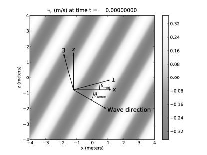
Fig. 1: Sample plane wave initial condition, showing the relation between the global $x-z$ axes, the material $1-3$ axes, and the wave propagation direction. For this plot $\theta_{\text{mat}}=15^{\circ}$ and $\theta_{\text{wave}}=-30^{\circ}$. The shading shows the $z$-direction solid matrix velocity. This plot depicts a fast P wave, with an angular frequency of $10^{4}$ rad/s, in the same orthotropic sandstone medium used for the inviscid convergence tests. The grid dimensions are $800\times 800$ cells.

For each test case, we measured the error by taking the energy norm on each cell of the difference between the numerically obtained cell value and the true solution at the cell center. We then applied the grid 1-, 2-, and max-norms to the energy norm error field to obtain an aggregate error norm. (The grid 1-norm used here is just the linear algebraic 1-norm divided by the number of grid cells; similarly, the grid 2-norm is the linear algebraic 2-norm divided by the square root of the number of grid cells.) For each combination of $\theta_{\text{wave}}$, $\theta_{\text{mat}}$, and wave family, we performed a linear least-squares fit of $\log(\text{error})$ versus $\log(m)$, where $m$ is the number of grid cells along each axis. The slope of this fit was considered to be the convergence rate of the code for this set of cases.

Table 2 summarizes the results of this convergence study. The convergence rates listed are the maximum, minimum, and mean over all combinations of $\theta_{\text{wave}}$ and $\theta_{\text{mat}}$; the worst $R^{2}$ value for the least-squares fit of $\log(\text{error})$ versus $\log(m)$ is also reported. The last two columns of Table 2 give the lowest and highest error for each wave in each norm on the finest grid, observed over all combinations of $\theta_{\text{wave}}$ and $\theta_{\text{mat}}$, normalized by the energy norm of the plane wave eigenvector $\mbox{$\mathbf{Q}$}_{0}$ formed from the vectors $\mathbf{V}_{0}$ and $\mathbf{T}_{0}$ of the preceding section in order to allow a fair comparison between different cases. We see second-order convergence in all three norms for the fast P and S waves. Results are impaired for the slow P-wave because its slow propagation speed causes it to be underresolved on the coarser grids at the frequency used, but we still observe second-order convergence in the 1-norm and 2-norm. While the error varies somewhat depending on the wave propagation and principal material directions, it does so by no more than a factor of 3-4, indicating that there are no severe grid alignment effects.

Table 2: Summary of convergence results for inviscid test cases

		Convergence rate				Error on $800\times 800$ grid
Wave family	Error norm	Best	Worst	Mean	Worst $R^{2}$ value	Best	Worst
Fast P	1-norm	2.03	2.01	2.01	0.99994	$2.53\times 10^{-5}$	$6.90\times 10^{-5}$
	2-norm	2.02	2.01	2.01	0.99995	$3.04\times 10^{-5}$	$8.23\times 10^{-5}$
	Max-norm	2.02	1.96	2.00	0.99943	$5.61\times 10^{-5}$	$1.76\times 10^{-4}$
S	1-norm	2.01	2.00	2.01	1.00000	$1.31\times 10^{-4}$	$3.23\times 10^{-4}$
	2-norm	2.01	2.00	2.00	1.00000	$1.49\times 10^{-4}$	$3.74\times 10^{-4}$
	Max-norm	2.00	1.96	1.99	0.99977	$2.80\times 10^{-4}$	$7.98\times 10^{-4}$
Slow P	1-norm	1.99	1.92	1.97	0.99922	$3.05\times 10^{-3}$	$1.13\times 10^{-2}$
	2-norm	1.99	1.94	1.97	0.99953	$3.44\times 10^{-3}$	$1.27\times 10^{-2}$
	Max-norm	1.93	1.67	1.80	0.99146	$8.81\times 10^{-3}$	$3.16\times 10^{-2}$

We do not include convergence results with wave limiting here, but informal exploration suggests that for the cases above, limiting reduces the order of accuracy to about 1.9 in the 1-norm, 1.8 in the 2-norm, and 1.6 in the max-norm. This is because wave limiting tends to clip extrema in order to avoid introducing spurious oscillations. Despite the reduced order of accuracy, however, using a limiter can improve actual error in many cases, often in the 1-norm but even in the max-norm if a wave is poorly resolved or heavily affected by dispersive errors. Figure 2 shows an example of the effect of limiting, using the Monotonized Centered (MC) limiter, on the normalized energy max-norm and 1-norm errors in each of the three wave families for the inviscid test cases with $\theta_{\text{mat}}=\theta_{\text{wave}}=0$. For each wave, the max-norm error decreases more slowly with increasing grid size when the limiter is present. The fast P wave is well resolved even on the coarsest grid, and always shows lower max-norm error without limiting. The S wave is somewhat less well-resolved, and the difference between the two curves is smaller, with the max-norm errors both with and without limiters roughly equal on the coarsest grid. Finally, the slow P wave starts out poorly resolved, and using a limiter produces lower max-norm error on all but the finest grid. The 1-norm error is lower with the limiter included for all cases. For further discussion of the benefits and drawbacks of using limiters, see LeVeque [36]. There have also been efforts to produce limiters that are compatible with higher-order methods; see for example Čada and Torrilhon [11], Liu and Tadmor [38], or the recent review by Kemm [35].

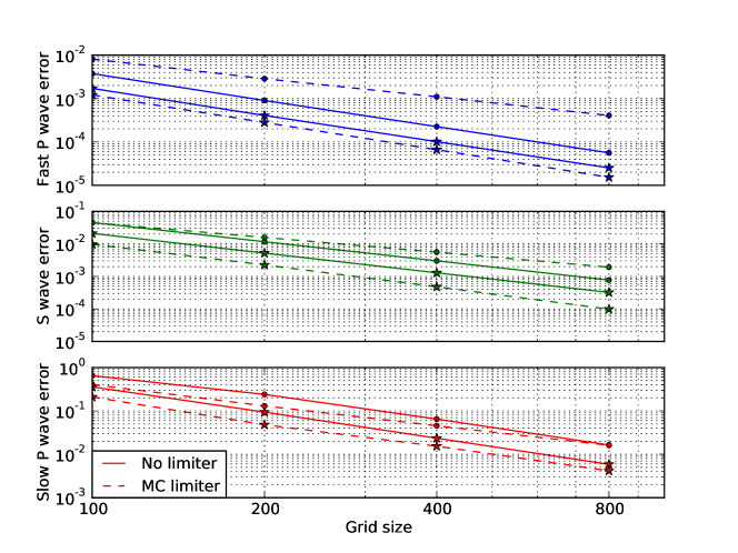
Fig. 2: Comparison of error both with and without a limiter for the inviscid plane wave test cases with $\theta_{\text{mat}}=\theta_{\text{wave}}=0$. The circles indicate normalized energy max-norm error, while the stars indicate normalized energy 1-norm error. The limiter is always beneficial in the 1-norm for these cases, and is also helpful in the max-norm for poorly-resolved waves.

4.3 Plane wave convergence results — viscous

With viscosity included, numerical solution of the equations of poroelasticity becomes substantially more challenging. The chief difficulty is that the dissipation term has its own associated time scales, independent of the computational grid. Since an appropriate time step for the wave propagation part of the system is proportional to the grid size — preferably with a CFL number near 1 — for large enough grid cell sizes the dissipation term is stiff relative to the wave propagation term. While we maintain stability by solving the dissipation term exactly, because the wave propagation and dissipation parts of the system do not commute, we can still heuristically expect problems in our operator splitting scheme if the time step is much longer than the characteristic time scale for dissipation.

Revisiting the subcharacteristic condition of section 3.3, Figure 3 shows the wave speeds for the full and reduced systems as a function of propagation direction relative to the principal axes. The strict subcharacteristic condition (61) is satisfied for all the materials we examine, although the reduced P wave speed nearly reaches the fast P wave speed for the glass/epoxy material. In fact, an even stricter condition is satisfied: the wave speeds interleave, with exactly one wave of the reduced system between each consecutive pair of waves of the full system. Based on the discussion of section 3.3, this suggests that we will not see spurious solutions or incorrect wave speeds from our numerical solution.

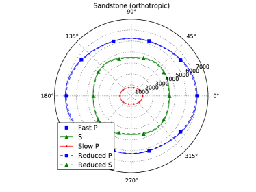
(a)

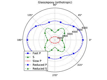
(b)

Fig. 3: Wave speeds (meters per second) for full and reduced systems for both materials used with viscosity included, as a function of propagation angle. Zero propagation angle corresponds to the material principal $1$-axis. The strict subcharacteristic condition (61) is satisfied.

To better explore the behavior of our numerical method in the presence of dissipation, we ran a series of numerical tests in the same sandstone medium as the inviscid test cases, against plane wave solutions at frequencies ranging from 10 Hz to 20 kHz. (The maximum frequency for low-frequency Biot theory to be valid in this medium is roughly 25 kHz.) For all cases, the material 1-axis was aligned with the global $x$-axis, and waves were set to propagate in the positive $x$ direction. For the fast P and S waves, we chose the domain size to be two damped wavelengths of the wave in question; since the slow P wave has a characteristic decay length (the distance over which the wave amplitude decreases by a factor of $e$) that is typically a fifth or less of its wavelength, we chose the domain size for the slow P wave cases to be twice the characteristic decay length instead. We chose the domain sizes in this way so that the number of grid cells per wavelength, or per decay length, would be constant across all frequencies; this keeps the discretization error contributed from the wave propagation part of the system roughly constant for each grid size across all frequencies, helping to isolate the error caused by operator splitting. The total simulation time for the fast P and S wave cases was 1.25 cycles of the wave (we chose a non-integer number of cycles to avoid any possible spoofing where an unchanged solution might appear correct), while for the slow P wave cases it was 1.25 times the time for a fast P wave traveling in the $x$ direction to cross the domain. For each combination of wave family and frequency, we computed solutions on grids of size $100\times 100$, $200\times 200$, $400\times 400$, and $800\times 800$, using both Godunov and Strang splitting.

Figure 4 shows the results of these tests in the same normalized energy max-norm used for the inviscid cases. There is a pronounced qualitative difference in convergence behavior depending on frequency. At low frequencies, corresponding to large grid cell sizes and long time steps, both splitting methods show first-order convergence. Starting at a step length of roughly 5-10 times the characteristic time $\tau_{d}$ for dissipation in the $x$ direction (the time over which the $x$ velocity of the fluid relative to the matrix decreases by a factor of $e$), the two methods begin behaving differently, with the Godunov splitting error increasing abruptly while the Strang splitting error sweeps smoothly down to second-order convergence. This effect is most visible for the fast P wave, but can also be seen slightly in the $400\times 400$ grid and strongly in the $800\times 800$ grid for the S wave. Because of the choice of domain size, the slow P test cases always had a time step below the characteristic dissipation time; they display consistent first-order convergence with Godunov splitting and second-order with Strang. The qualitative shift in behavior with time step length can be understood by noting that for a time step much longer than the characteristic time, the solution operator $\exp(\mbox{$\mathbf{D}$}\Delta t)$ of the dissipative part of the system is essentially a projection operator that sets the fluid relative velocity to zero and transfers all of the fluid relative momentum into the bulk motion of the medium. The effect of this projection operator is essentially the same whether it is applied once per time step after solution of the wave propagation part of the system (Godunov splitting), or twice, both before and after wave propagation (Strang splitting).

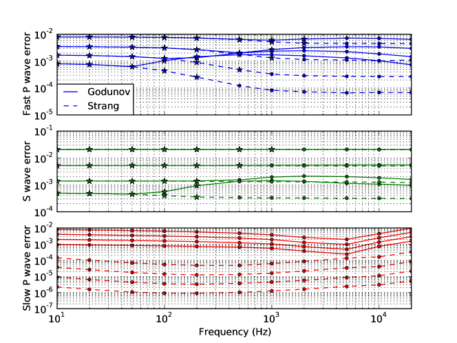
Fig. 4: Normalized energy max-norm error for operator splitting tests. For each splitting method (Godunov or Strang) within each subplot, the curves fall in order of increasing grid fineness, with each curve from a grid twice as fine as the curve above. The top curve is on a $100\times 100$ grid, and the bottom is on an $800\times 800$. The circles indicate where the time step was less than the characteristic time scale $\tau_{d}$ for dissipation in the $x$ direction; the stars indicate where the time step was greater.

With these results available to inform our choices, we conducted a set of convergence studies similar to the inviscid cases in the previous subsection. Because of the qualitative difference in convergence behavior for different time step regimes, we performed convergence studies both at a point in the high-frequency convergence regime of Figure 4 (10 kHz), and at a low-frequency point (10 Hz). Since the slow P wave decays extremely rapidly in the presence of viscosity — typically by a factor of 10 to 100 or more per wavelength in the valid frequency range for Biot theory — we chose a different domain size for the viscous slow P test cases. For the high-frequency cases, we chose square domains with side length 1.2 meters for the fast P and S waves — roughly two wavelengths of the fast P wave at 10 kHz — and 5 centimeters for the slow P wave — roughly 2-5 times the characteristic decay length for this wave, depending on propagation direction in the orthotropic medium. For the low-frequency cases, the domain size was 1200 meters for the fast P and S waves, and 1 meter for the slow P wave — again, 2-4 times the characteristic decay length, which is far shorter than the wavelength. This huge disparity in domain sizes is somewhat troublesome, but it is not clear whether simulation results for a slow P wave on a domain of the size used for the fast P and S waves would be meaningful, since the solution decays over such a short distance. For practical problems, this would be an excellent opportunity for adaptive mesh refinement, to generate fine grids where and when slow P waves appear, then coarsen the grid again after they dissipate.

We ran all of the viscous test cases to essentially the same final times as for the frequency sweep of Figure 4. For the $10\,\text{kHz}$ runs, this was $125\,\text{$\mu$s}$ for the fast P and S waves (1.25 periods of the wave), and $10.4\,\text{$\mu$s}$ for the slow P wave (1.25 times the time for a fast P wave to cross the domain), while for the $10\,\text{Hz}$ runs it was $0.125\,\text{s}$ for the fast P and S waves, and $208\,\text{$\mu$s}$ for the slow P wave. Strang splitting was used for all cases. All other aspects of the solution, including the sets of wave propagation and material principal directions $\theta_{\text{wave}}$ and $\theta_{\text{mat}}$ as well as the method of setting the boundary condtions, were the same as for the inviscid test cases, and we measured the solution error using the same set of norms.

Table 3 summarizes convergence for the high-frequency viscous cases. We again see consistent second-order convergence in all norms for the fast P and S waves at high frequency, and a similar amount of dependence of error on wave propagation direction. For the slow P wave at high frequency, however, results are substantially different from the inviscid cases. We see second-order convergence, since the solution is well-resolved on the grids used here, but there is now a factor of several hundred difference between the maximum and minimum error at a single grid size. Close examination of the error for individual cases shows that it is primarily a function of the offset $\theta_{\text{wave}}-\theta_{\text{mat}}$; for a fixed value of $\theta_{\text{wave}}-\theta_{\text{mat}}$ and a fixed grid size, the error is similar across all values of $\theta_{\text{mat}}$. This indicates that the large variation in error is a effect of the alignment of the wavefront relative to the principal material axes, rather than a grid alignment effect. The likely cause is the substantial difference in the characteristic decay times between the 1 and 3 axes of the material — the decay time in the 1 direction is 5.95 microseconds, while in the 3 direction it is 1.82 microseconds. This large variation in decay time causes a large variation in the operator splitting error. In addition, the characteristic decay length is substantially shorter in the 3 direction, causing the solution magnitude to be larger at the “upstream” (opposite the propagation direction) edge of the domain relative to the value at the center against which the error is normalized; the larger solution magnitude naturally results in a larger error.

Table 3: Summary of convergence results for viscous, high-frequency test cases

		Convergence rate				Error on $800\times 800$ grid
Wave family	Error norm	Best	Worst	Mean	Worst $R^{2}$ value	Best	Worst
Fast P	1-norm	2.03	2.01	2.01	0.99996	$2.61\times 10^{-5}$	$7.31\times 10^{-5}$
	2-norm	2.03	2.01	2.01	0.99996	$3.16\times 10^{-5}$	$8.79\times 10^{-5}$
	Max-norm	2.05	2.00	2.02	0.99887	$6.44\times 10^{-5}$	$1.77\times 10^{-4}$
S	1-norm	2.01	2.01	2.01	1.00000	$1.38\times 10^{-4}$	$3.39\times 10^{-4}$
	2-norm	2.01	2.00	2.01	1.00000	$1.58\times 10^{-4}$	$3.98\times 10^{-4}$
	Max-norm	2.03	1.99	2.00	0.99978	$2.99\times 10^{-4}$	$7.59\times 10^{-4}$
Slow P	1-norm	2.01	2.00	2.01	1.00000	$2.12\times 10^{-6}$	$1.74\times 10^{-4}$
	2-norm	2.02	2.00	2.01	1.00000	$2.49\times 10^{-6}$	$3.26\times 10^{-4}$
	Max-norm	2.02	1.96	2.00	0.99988	$6.53\times 10^{-6}$	$2.25\times 10^{-3}$

Table 4 shows the results for the low-frequency viscous test cases. The fast P and S waves again show only a weak dependence of error on wave propagation and principal material direction, but their convergence rates are substantially degraded, just as in the low-frequency range of Figure 4. Convergence of the fast P wave is roughly first-order in the worst case, due to the long time step relative to the characteristic decay times. Surprisingly, results for the S wave are only slightly better in the worst case, likely due to the much shorter characteristic decay time in the 3 direction. If the grid were further refined, we would presumably reach a second-order convergence regime as the time step approached the characteristic decay time, but in order to have a time step similar to the shortest decay time at a CFL number of 0.9 we would need a grid cell size of roughly $13\,\text{cm}$ — resulting in a $90000\times 90000$ cell grid on the $1200\,\text{m}$ square domain if this size is uniform! The low-frequency slow P wave cases, by contrast, show the same strong dependence of error on the alignment of the wave direction with the principal material direction as the high-frequency cases, but because the domain size was much smaller and the time step much shorter, we observe consistent second-order convergence.

Table 4: Summary of convergence results for viscous, low-frequency test cases

		Convergence rate				Error on $800\times 800$ grid
Wave family	Error norm	Best	Worst	Mean	Worst $R^{2}$ value	Best	Worst
Fast P	1-norm	1.57	1.10	1.26	0.99239	$1.95\times 10^{-4}$	$4.24\times 10^{-4}$
	2-norm	1.60	1.10	1.28	0.99206	$2.15\times 10^{-4}$	$4.77\times 10^{-4}$
	Max-norm	1.61	1.10	1.32	0.99014	$3.90\times 10^{-4}$	$1.04\times 10^{-3}$
S	1-norm	1.85	1.37	1.58	0.99241	$4.37\times 10^{-4}$	$7.30\times 10^{-4}$
	2-norm	1.85	1.37	1.59	0.99274	$5.01\times 10^{-4}$	$8.30\times 10^{-4}$
	Max-norm	1.83	1.36	1.58	0.98917	$9.63\times 10^{-4}$	$1.92\times 10^{-3}$
Slow P	1-norm	2.00	1.94	1.98	0.99985	$1.04\times 10^{-6}$	$4.88\times 10^{-5}$
	2-norm	2.03	1.93	1.99	0.99982	$1.08\times 10^{-6}$	$7.40\times 10^{-5}$
	Max-norm	2.09	1.84	1.98	0.99795	$2.40\times 10^{-6}$	$4.59\times 10^{-4}$

As a final comment on convergence, we note that while the rate of reduction of error with decreasing mesh size is poorer for the low-frequency fast P and S wave cases, this may not be a problem in practice unless very high accuracy is desired. For both frequency ranges investigated, the relative error in all three norms on the $800\times 800$ grid never exceeds $1.04\times 10^{-3}$ for the fast P wave, or $1.92\times 10^{-3}$ for the S wave — despite the numerical difficulties encountered, the waves are still well-resolved.

4.4 Single-material point source results

With the accuracy of our method characterized for simple plane wave solutions, we are able to move on to more interesting problems. First, we compare against the results of de la Puente et al. [23] and Carcione [12] for a point source in a uniform orthotropic medium. We used the orthotropic sandstone and glass/epoxy media described in Table 1; in both cases, the material 1 axis coincided with the $x$ axis. All test cases started with initial condition $\mbox{$\mathbf{Q}$}(x,z,0)=0$, and the domain was excited by a point source with a Ricker wavelet profile having peak frequency $f_{\text{src}}=3730\,\text{Hz}$ for sandstone and $3135\,\text{Hz}$ for glass/epoxy, acting with peak intensity $+1\,\text{Pa}\cdot\text{m}^{2}/\text{s}$ on the vertical normal stress $\sigma_{zz}$ and $-1\,\text{Pa}\cdot\text{m}^{2}/\text{s}$ on fluid pressure. The peak of the wavelet occurred $0.4\,\text{ms}$ after the start of the simulation. For each case, we used a square domain $18.7\,\text{m}$ on a side; the point source was placed at the center of the domain. The simulation time span was $1.56\,\text{ms}$ for the sandstone medium, and $1.80\,\text{ms}$ for glass/epoxy. We calculated results both with and without viscosity present.

We carried out all of these simulations on a uniform $501\times 501$ cell grid. The odd number of grid cells in each axis allowed us to apply the point source to a single grid cell. A grid resolution this high was necessary to resolve the slow P wave well; as in the plane wave test cases, the fast P and S waves were well-resolved on substantially coarser grids. The point source was implemented numerically as part of the source step in the operator splitting scheme; since the point source acts on stress variables, and the viscous dissipation acts on velocity variables, it does not matter which is applied first. The CFL number for all simulations was 0.9, resulting in 279 timesteps being taken for the sandstone case and 282 for the glass/epoxy. We used the monotonized centered (MC) limiter here — even though most of the solution is smooth, without a limiter the lack of smoothness at the source point produces substantial spurious oscillations in the solution. Figure 5 shows the results of these simulations. These figures correspond to Figures 6 and 7 of de la Puente et al. [23], or Figures 5 and 7 of Carcione [12], and are in agreement with them.

(a)

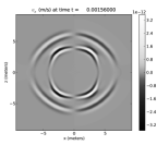
(b)

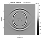
(c)

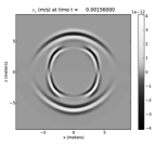
(d)

(e)

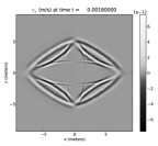
(f)

(g)

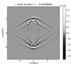
(h)

Fig. 5: Results for point source test cases. Top: sandstone; bottom: glass/epoxy; left to right: $v_{x}$ without viscosity, $v_{x}$ with viscosity, $v_{z}$ without viscosity, $v_{z}$ with viscosity.

4.5 Heterogeneous domain results

We conclude our results here with a wave reflection and interconversion problem that demonstrates the ability of our code to model material interfaces, as well as the benefits of using adaptive mesh refinement — a feature of the amrclaw variant of clawpack that we have not used thus far.

Our final test case is a large-scale inviscid problem with a bed of isotropic shale overlying isotropic sandstone, with material properties given in Table 1. The problem domain is the rectangle $[0,1500\,\text{m}]\times[0,1400\,\text{m}]$ in the $x$-$z$ plane, with the boundary between the materials at $z=700\,\text{m}$. There is a point source at $(x,z)=(750\,\text{m},900\,\text{m})$, again with a Ricker wavelet profile in time, with peak frequency $50\,\text{Hz}$. The source acts on the $z$-direction normal stress and fluid pressure with peak intensities $+2.3\times 10^{13}\,\text{Pa}\cdot\text{m}^{2}/\text{s}$ and $-2.3\times 10^{13}\,\text{Pa}\cdot\text{m}^{2}/\text{s}$, respectively, similarly to the previous test cases in homogeneous domains. This source magnitude was chosen to match the magnitude of the response shown by de la Puente et al. [23]. The peak of the source was delayed $40\,\text{ms}$ after the start of the simulation, and the total duration of the run was $0.5\,\text{s}$. In addition to time-snapshots of the solution at particular instants, we also recorded solution time histories at three “gauges”, located at $(x_{1},z_{1})=(950\,\text{m},750\,\text{m})$, $(x_{2},z_{2})=(950\,\text{m},650\,\text{m})$, and $(x_{3},z_{3})=(950\,\text{m},500\,\text{m})$.

For our adaptively refined simulation, the coarsest-level computational grid was $75\times 70$ cells in size, giving square cells $20\,\text{m}$ on a side. We used two additional levels of refinement on this grid, the first at a factor of $4$, and the second at further factor of $6$, so that cells on the finest grids were $0.83\,\text{m}$ on a side. Our code flagged a cell for mesh refinement when the energy norm (using the material properties of that cell) of the difference $\Delta\mbox{$\mathbf{Q}$}$ between its state vector and that of any adjacent cell exceeded $32.5\,\text{J}^{1/2}/\text{m}^{3/2}$, with the exception of the rectangle $[700\,\text{m},1000\,\text{m}]\times[450\,\text{m},950\,\text{m}]$, where the threshold for refinement was lowered to $3.25\,\text{J}^{1/2}/\text{m}^{3/2}$ in order to improve accuracy at the gauges. These tolerances were chosen empirically based on the observed magnitude of the waves in the simulation. This refinement criterion is a generalization of the typical amrclaw approach of refining based on the difference between the solution values in neighboring cells, which has been used successfully on many problems; amrclaw makes it easy to set alternate user-specified refinement criteria if desired, and also offers automatic error estimation via Richardson extrapolation. Besides refinement based on the solution field, the source location was also flagged for refinement to the finest level available whenever the source intensity was greater than about $10^{-9}$ of peak. Since the grid size was even in each direction on all but the coarsest grids, the source was distributed over the four cells closest to its location using a bilinear weighting. We again used the MC limiter for this problem.

Figure 6 shows a snapshot of the $z$-direction solid velocity $0.25\,\text{s}$ after the start of the simulation, analogous to Figure 9(a) of de la Puente et al. [23], along with the AMR grids at this time. The solid black dot indicates the source location, and the white-centered black dots indicate the gauge locations. Because the eigenvectors associated with each wave family are different in the two materials, when a wave impinges on the material interface it produces reflected and transmitted waves in each of the three families; this results in a rich and complex solution structure. In addition to the reflected and transmitted waves, we also see head waves, where a wave in the lower half of the domain excites a slower wave family in the upper half. This results in a straight wavefront, rather than a curved one. At this point in the simulation the level 2 AMR grids have expanded to cover most of the domain, but the level 3 grids are concentrated around the wavefronts. Figure 7 shows the time histories of the solid $x$ and $z$ velocities at the three gauges. The results are in generally good agreement with Figure 10 of de la Puente et al. [23], also shown in Figure 7, although the peaks of slow P wave event at $t=0.45\,\text{s}$ at gauge 3 are clipped in our simulation because of the limiter, and the magnitude of the second large excursion in vertical velocity at gauge 3 in our solution seems somewhat less.

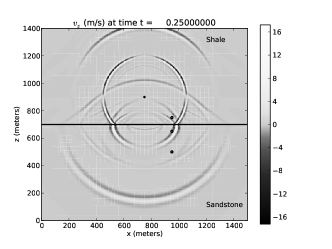
(a)

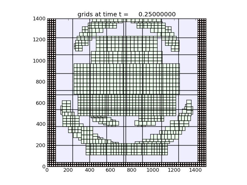
(b)

Fig. 6: Left: snapshot of $z$-direction solid velocity 0.25 seconds after the start of the simulation. The source location is marked with a solid black dot, while the gauges are marked with white-centered black dots. The gauges are numbered from top to bottom. Right: AMR grids at this time point. Individual cells are drawn on the coarsest AMR level, but only grid outlines are shown on finer levels.

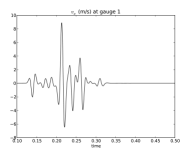
(a)

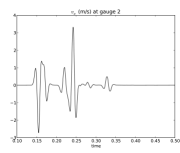
(b)

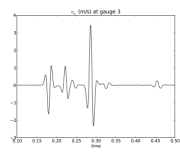
(c)

(d)

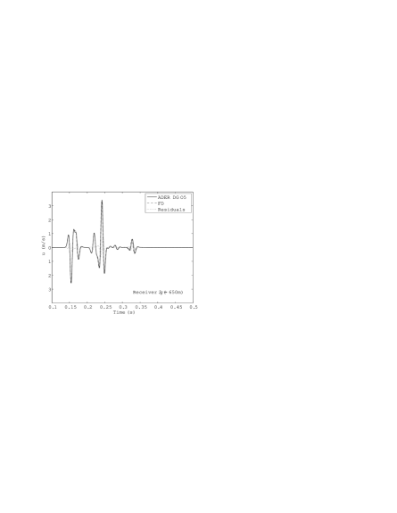
(e)

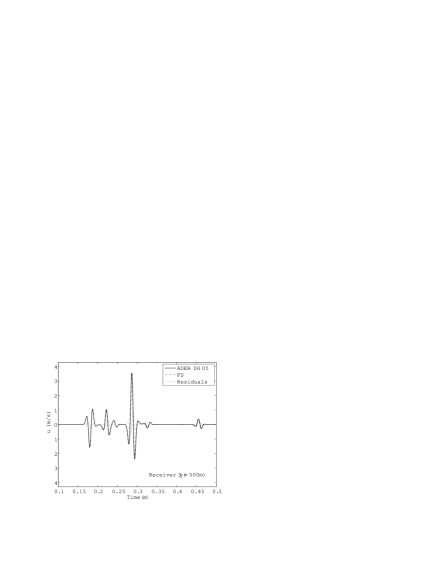
(f)

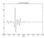
(g)

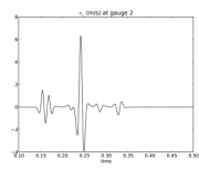
(h)

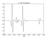
(i)

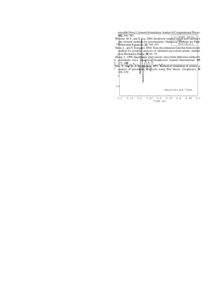
(j)

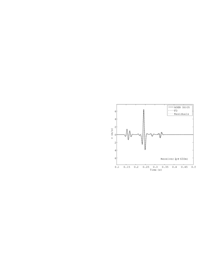
(k)

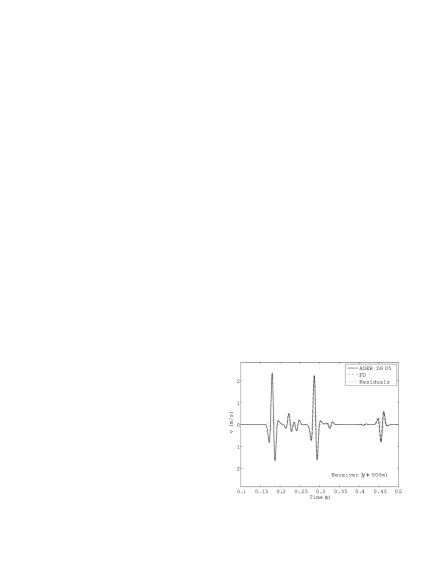
(l)

Fig. 7: Time-histories of solid velocity at the gauges indicated in Figure 6a. Top to bottom: $x$-direction from clawpack; $x$-direction from de la Puente et al. [23]; $z$-direction from clawpack; $z$-direction from de la Puente et al. Left to right: gauge 1, at $(x,z)=(950\,\text{m},750\,\text{m})$; gauge 2, at $(950\,\text{m},650\,\text{m})$; gauge 3, at $(950\,\text{m},500\,\text{m})$. Results of de la Puente et al. are reproduced in accordance with the policies of the publishing journal; the ADER-DG and FD curves in these plots are discontinuous Galerkin and finite difference results, respectively.

While the variety of different wave speeds and reflected/transmitted waves in this problem make adaptive mesh refinement less useful than is typically the case — by halfway through the simulation time, Figure 6b shows a large portion of the domain refined at the finest level, because there are wavefronts present throughout the domain — we still realize a substantial savings in computation time. On an Amazon EC2 Cluster 8XL instance, running with 32 OpenMP threads, these results took 20 minutes 31 seconds to obtain, whereas a uniformly refined grid with the same cell size as the finest AMR grids took 47 minutes 19 seconds and produced no significant change in the solution. (Both times are the average of two runs; each pair differed by 4 seconds or less.) The large number of hardware threads available on this type of EC2 instance is the reason why there are so many separate fine grids in Figure 6b — amrclaw uses a coarse-grained parallelization strategy, with each grid at each time step processed by a single thread, which means that many grids must be present in order to take full advantage of highly parallel computers. The number of grids used at each refinement level is indirectly controlled by setting the maximum size of the individual grids; for the AMR computation shown above, grids were allowed to extend no more than 60 cells in any direction. Having a very large number of small grids (1047 level 3 grids in the figure) also eases load balancing between threads, since most grids are of similar size, and each thread processes many grids.

5 Summary and Conclusions

We have demonstrated a high-resolution finite volume code for modeling wave propagation in porous media using Biot poroelasticity theory, with the ability to model inhomogeneous domains and use adaptive mesh refinement to improve solution accuracy at substantially lower computational cost than for a uniformly refined grid. We included the dissipative source term in Biot’s equations using operator splitting. While this technique has produced spurious solutions when applied to certain types of stiff source terms in the past, we have presented an heuristic argument, based on the wave speeds of a reduced system satisfying a certain subcharacteristic condition, that we should not expect to encounter spurious solutions here. This expectation was borne out by our numerical results.

For the inviscid and viscous high-frequency regimes, our numerical solutions converge to analytic plane wave solutions for fast P and S waves with second-order accuracy. Convergence rates were somewhat impaired for the inviscid slow P wave cases tested due to the short wavelength at the frequency chosen, which caused the waves to be underresolved on the coarsest grids. However, the viscous, high-frequency slow P wave test cases showed unambiguous second-order convergence, which indicates that we can also expect second order in the inviscid case when the slow P wave is well-resolved. Due to the relative stiffness of the source term compared to the problem timescale for low-frequency waves, we obtained only roughly first-order accuracy for fast P and S waves in the low-frequency viscous regime. We obtained second-order accuracy for low-frequency slow P waves, but the slow P test cases were not directly comparable to the fast P and S cases. The other test cases examined, involving results for a point source in either a homogeneous orthotropic medium, or in a layered bed of two distinct isotropic media, agreed well with results for the same test cases published by other authors.

There are substantial opportunities for future work based on what we have presented here. One possibility is the extension of the finite volume methods used here to logically rectangular mapped grids. This extension is straightforward, and allows modeling of more complex domains with internal boundaries, so long as a (not necessarily smooth) mapping function can be found that maps the internal and external boundaries to rectangles in the computational domain. Another opportunity for future work is the implementation of a more accurate solution procedure at low frequencies, such as one based on the methods discussed by Hittinger [34] or Pember [42]. We intend to explore both these avenues in subsequent publications, along with applying the software developed here to some specific problems.

To aid in the reproducibility of the results presented here, we provide all of the code used to generate them at https://bitbucket.org/grady_lemoine/poro-2d-cartesian-archive.

References

- [1] E. Anderson, Z. Bai, C. Bischof, S. Blackford, J. Demmel, J. Dongarra, J. Du Croz, A. Greenbaum, S. Hammarling, A. McKenney, and D. Sorensen, LAPACK Users’ Guide, Society for Industrial and Applied Mathematics, Philadelphia, PA, third ed., 1999.
- [2] Keith Attenborough, David L. Berry, and Yu Chen, Acoustic scattering by near-surface inhomogeneities in porous media., tech. report, Defense Technical Information Center OAI-PMH Repository [http://stinet.dtic.mil/oai/oai] (United States), 1998.
- [3] M. J. Berger and R. J. LeVeque, Adaptive mesh refinement using wave-propagation algorithms for hyperbolic systems, SIAM Journal on Numerical Analysis, 35 (1998), pp. 2298–2316.
- [4] M. A. Biot, Theory of propagation of elastic waves in a fluid-saturated porous solid. I. Low-frequency range, Journal of the Acoustical Society of America, 28 (1956), pp. 168–178.
- [5] , Theory of propagation of elastic waves in a fluid-saturated porous solid. II. Higher frequency range, Journal of the Acoustical Society of America, 28 (1956), pp. 179–191.
- [6] , Mechanics of deformation and acoustic propagation in porous media, Journal of Applied Physics, 33 (1962), pp. 1482–1498.
- [7] James L. Buchanan and Robert P. Gilbert, Determination of the parameters of cancellous bone using high frequency acoustic measurements, Mathematical and Computer Modelling, 45 (2007), pp. 281–308.
- [8] , Determination of the parameters of cancellous bone using high frequency acoustic measurements II: inverse problems, Journal of Computational Acoustics, 15 (2007), pp. 199–220.
- [9] James L. Buchanan, Robert P. Gilbert, and Khaldoun Khashanah, Determination of the parameters of cancellous bone using low frequency acoustic measurements, Journal of Computational Acoustics, 12 (2004), pp. 99–126.
- [10] J. L. Buchanan, R. P. Gilbert, A. Wirgin, and Y. S. Xu, Marine acoustics: direct and inverse problems, SIAM, Philadelphia, 2004.
- [11] M. Čada and M. Torrilhon, Compact third-order limiter functions for finite volume methods, Journal of Computational Physics, 228 (2009), pp. 4118–4145.
- [12] J. M. Carcione, Wave propagation in anisotropic, saturated porous media: plane-wave theory and numerical simulation, Journal of the Acoustical Society of America, 99 (1996), pp. 2655–2666.
- [13] J. M. Carcione, Wave Fields in Real Media: Wave Propagation in Anisotropic, Anelastic, and Porous Media, Elsevier, Oxford, 2001.
- [14] J. M. Carcione, C. Morency, and J. E. Santos, Computational poroelasticity – a review, Geophysics, 75 (2010), pp. 75A229–75A243.
- [15] J. M. Carcione and G. Quiroga-Goode, Some aspects of the physics and numerical modeling of Biot compressional waves, Journal of Computational Acoustics, 3 (1995), pp. 261–280.
- [16] G.-Q. Chen, C. D. Levermore, and T.-P. Liu, Hyperbolic conservation laws with stiff relaxation terms and entropy, Communications in Pure and Applied Mathematics, 47 (1994), pp. 787–830.
- [17] G. Chiavassa and B. Lombard, Time domain numerical modeling of wave propagation in 2D heterogeneous porous media, Journal of Computational Physics, 230 (2011), pp. 5288–5309.
- [18] P. Colella, A. Majda, and V. Roytburd, Theoretical and numerical structure for reacting shock waves, SIAM Journal on Scientific and Statistical Computing, 7 (1986), pp. 1059–1080.
- [19] S. C. Cowin, Bone poroelasticity, Journal of Biomechanics, 32 (1999), pp. 217–238.
- [20] S. C. Cowin and L. Cardoso, Fabric dependence of bone ultrasound, Acta of Bioengineering and Biomechanics, 12 (2010).
- [21] S. C. Cowin and M. M. Mehrabadi, Identification of the elastic symmetry of bone and other materials, Journal of Biomechanics, 22 (1989), pp. 503–515.
- [22] N. Dai, A. Vafidis, and E. Kanasewich, Wave propagation in heterogeneous porous media: a velocity-stress, finite-difference method, Geophysics, 60 (1995), pp. 327–340.
- [23] J. de la Puente, M. Dumbser, M. Käser, and H. Igel, Discontinuous Galerkin methods for wave propagation in poroelastic media, Geophysics, 73 (2008), pp. T77–T97.
- [24] G. Degrande and G. De Roeck, FFT-based spectral analysis methodology for one-dimensional wave propagation in poroelastic media, Transport in Porous Media, 9 (1992), pp. 85–97.
- [25] H. Deresiewicz and R. Skalak, On uniqueness in dynamic poroelasticity, Bulletin of the Seismological Society of America, 53 (1963), pp. 783–788.
- [26] E. Detournay and A. H-D. Cheng, Poroelastic response of a borehole in a non-hydrostatic stress field, International Journal of Rock Mechanics and Mining Sciences and Geomechanics Abstracts, 25 (1988), pp. 171–182.
- [27] S. K. Garg, A. H. Nayfeh, and A. J. Good, Compressional waves in fluid-saturated elastic porous media, Journal of Applied Physics, 45 (1974), pp. 1968–1974.
- [28] R. F. Gibson, Principles of Composite Material Mechanics, McGraw-Hill, New York, 1994.
- [29] R. P. Gilbert, P. Guyenne, and M. Yvonne Ou, A quantitative ultrasound model of the bone with blood as the interstitial fluid, Mathematical and Computer Modelling, 55 (2012), pp. 2029–2039.
- [30] R. P. Gilbert and Z. Lin, Acoustic field in a shallow, stratified ocean with a poro-elastic seabed, Zeitschrift für Angewandte Mathematik und Mechanik, 77 (1997), pp. 677–688.
- [31] R. P. Gilbert and M. Yvonne Ou, Acoustic wave propagation in a composite of two different poroelastic materials with a very rough periodic interface: a homogenization approach, International Journal for Multiscale Computational Engineering, 1 (2003).
- [32] Boris Gurevich and Michael Schoenberg, Interface conditions for Biot’s equations of poroelasticity, Journal of the Acoustical Society of America, 105 (1999), pp. 2585–2589.
- [33] S. Hassanzadeh, Acoustic modeling in fluid-saturated porous media, Geophysics, 56 (1991), pp. 424–435.
- [34] J. A. Hittinger, Foundations for the generalization of the Godunov method to hyperbolic systems with stiff relaxation source terms, PhD thesis, University of Michigan, 2000.
- [35] F. Kemm, A comparative study of TVD-limiters – well-known limiters and an introduction of new ones, International Journal for Numerical Methods in Fluids, 67 (2011), pp. 404–440.
- [36] R. J. LeVeque, Finite Volume Methods for Hyperbolic Problems, Cambridge University Press, New York, 2002.
- [37] R. J. LeVeque and H. C. Yee, A study of numerical methods for hyperbolic conservation laws with stiff source terms, Journal of Computational Physics, 86 (1990), pp. 187–210.
- [38] X.-D. Liu and E. Tadmor, Third order nonoscillatory central scheme for hyperbolic conservation laws, Numerische Mathematik, 79 (1998), pp. 397–425.
- [39] B. G. Mikhailenko, Numerical experiment in seismic investigations, Journal of Geophysics, 58 (1985), pp. 101–124.
- [40] C. Morency and J. Tromp, Spectral-element simulations of wave propagation in porous media, Geophysical Journal International, 179 (2008), pp. 1148–1168.
- [41] R. B. Pember, Numerical methods for hyperbolic conservation laws with stiff relaxation I. Spurious solutions, SIAM Journal on Applied Mathematics, 53 (1993), pp. 1293–1330.
- [42] , Numerical methods for hyperbolic conservation laws with stiff relaxation II. Higher-order Godunov methods, SIAM Journal on Scientific Computing, 14 (1993), pp. 824–859.
- [43] J. E. Santos and E. J. Oreña, Elastic wave propagation in fluid-saturate porous media, part II: The Galerkin procedures, Mathematical Modeling and Numerical Analysis, 20 (1986), pp. 129–139.
- [44] M. D. Sharma, Wave propagation across the boundary between two dissimilar poroelastic solids, Journal of Sound and Vibration, 314 (2008), pp. 657–671.
- [45] The clawpack authors, clawpack software. www.clawpack.org.