Skewness as a probe of Baryon Acoustic Oscillations

Abstract

In this study we show that the skewness $S_{3}$ of the cosmic density field contains a significant and potentially detectable and clean imprint of Baryonic Acoustic Oscillations. Although the BAO signal in the skewness has a lower amplitude than second order measures like the two-point correlation function and power spectrum, it has the advantage of a considerably lower sensitivity to systematic influences. Because it lacks a direct dependence on bias if this concerns simple linear bias, skewness will be considerably less beset by uncertainties due to galaxy bias. Also, it has a weaker sensitivity to redshift distortion effects. We use perturbation theory to evaluate the magnitude of the effect on the volume-average skewness, for various cosmological models. One important finding of our analysis is that the skewness BAO signal occurs at smaller scales than that in second order statistics. For an LCDM spectrum with WMAP7 normalization, the BAO feature has a maximum wiggle amplitude of $~{}3\%$ and appears at a scale of $\sim 82h^{-1}\,{\rm Mpc}$. We conclude that the detection of BAO wiggles in future extensive galaxy surveys via the skewness of the observed galaxy distribution may provide us with a useful, and potentially advantageous, measure of the nature of Dark Energy.

1 Introduction

We live in the era of precision cosmology. The last twenty years of tremendous progress in astronomical observations allowed us to establish the standard cosmological model, the Lambda Cold Dark Matter model (LCDM). The cosmological parameters characterising the model have been determined to an accuracy of better than a percent.

Notwithstanding the success of these measurements, we are left puzzled at finding a universe whose dynamics and fate are dominated by a dark energy whose identity remains a mystery. It is not even sure whether it really concerns an energy component to be associated to a new species in the Universe, a cosmological constant or a modification of gravity itself. It is far from trivial to constrain the nature of dark energy, due to the relatively weak imprint of the equation of state of dark energy, in combination with sizeable observational errors (Frieman et al., 2008). Its principal influence is the way in which it affects the expansion of the Universe. In turn, this determines the growth of the cosmic density perturbations.

Since the discovery of the accelerated expansion of the universe on the basis of the luminosity distance of supernovae (Riess et al., 1998; Perlmutter et al., 1999), a range of alternative probes have provided additional constraints on the nature of dark energy. The temperature perturbations in the cosmic microwave background, weak gravitational lensing by the large scale matter distribution and the structure formation growth rate are well-known examples of dark energy probes.

The particular probe that we wish to address in this study are baryonic acoustic oscillations (BAOs), the residual leftover in the baryonic and dark matter mass distribution of the primordial sound waves in the photon-baryon plasma in the pre-recombination universe. Following the decoupling between matter and radiation, the primordial sound waves devolve into slight and subtle wiggles in the distribution of galaxies, the ”baryonic wiggles” (Peebles & Yu, 1970; Sunyaev & Zeldovich, 1970). These have a characteristic size in the order of the sound horizon at decoupling or, more accurately, the baryon drag epoch at which baryons are released from the Compton drag of photons. The value of the latter is around $\sim 150h^{-1}\,{\rm Mpc}$ for the standard LCDM cosmology.

The BAO wiggles were first detected in the power spectrum of galaxies in the 2dFGRS (Cole et al., 2005) and in the in the two-point correlation function of the SDSS galaxy redshift surveys (Eisenstein et al., 2005). In the meantime, this has been followed up by a flurry of studies (e.g. Tegmark et al., 2006; Hütsi, 2006; Percival et al., 2007; Padmanabhan et al., 2007), and have led to the initiation of a number of large observational program. Notable examples of surveys that (partially) probe dark energy by means of Baryonic Acoustic Oscillations are WiggleZ (Drinkwater et al., 2010), BOSS (Ross et al., 2010) and the Dark Energy Survey, along with the ambitious ESA Euclid Mission project (Laureijs et al., 2011).

The basic idea behind the use of BAOs as probe of dark energy is to use the sound horizon at decoupling as a standard ruler. Its physical size is known precisely from first principle, and its angular size was measured accurately in the angular spectrum of the microwave background temperature anisotropies. By assessing the size of the BAO characteristic scale over a range of (lower) redshifts, we may directly measure the angular diameter distance as a function of z, and hence constrain the nature of dark energy. The BAO scale can be inferred from the imprint of the sound horizon in the spatial distribution of galaxies, and can be inferred from the correlation function, power spectrum or other measures of spatial clustering (Eisenstein et al., 1998; Cooray et al., 2001; Hu & Haiman, 2003; Blake & Glazebrook, 2003; Seo & Eisenstein, 2003; Zhan & Knox, 2006). It was also suggested that the BAO signature could be measured with a use of higher order statistics. However this mainly concentrated on bispectrum or three-point function alone (Sefusatti et al., 2006; Gaztañaga et al., 2009). Albeit, while the theoretical underpinning of BAOs is quite straightforward, the practical limitations and complications are considerable. A range of systematic effects, ranging from non-linearities to redshift space distortions and unknown galaxy biasing effects, severely complicates the analysis.

To alleviate some of the practical complications, in this paper we advocate the idea to look for the BAO wiggles in the reduced third moment of the density field, the skewness $S_{3}$. According to perturbation theory, the $S_{3}$ is sensitive to second-order logarithmic derivative of the matter power spectrum P(k). The direct implication of this is the imprint of the BAO wiggles in the skewness. This forms a potentially powerful means of probing the baryonic acoustic oscillations. Unlike the more conventional second order probes, i.e. two-point correlation function and power spectrum, the skewness is insensitive to the bias of galaxies in case this involves simple linear or local bias. As important is the fact that skewness has been found to be rather marginally affected, in comparison to two-point correlation function or power spectrum, by redshift space distortions (Bouchet et al., 1992; Hivon et al., 1995; Bouchet et al., 1995).

These observations suggest that the skewness may offer a cleaner probe of the baryonic acoustic oscillations in the galaxy distribution, less ridden by the systematic uncertainties that still beset the present BAO experiments. In this study, we present the basic results for measuring the signature and scale of baryonic acoustic oscillations. We assess the BAO signature in the skewness of the cosmic matter density field, by invoking the theoretical power spectrum for a universe filled with a given baryonic fraction of matter. In § 2 we present the perturbation theoretical basis of the use of skewness as BAO probe, including a discussion of the influence of non-linearities on the skewness estimates. This is followed by a presentation of the results in § 3 towards the feasibility of relating the skewness to the scale and amplitude of the BAO. Prospects and complications are discussed in § 4.

2 BAO in weakly non-linear perturbation theory

In this section we first outline the basic perturbation theory concepts underlying our BAO analysis, followed by a presentation of the formalism to incorporate the baryonic acoustic signatures in the power spectrum to evaluate the skewness $S_{3}$ of the field.

2.1 Skewness and Perturbation Theory

In our discussion on the skewness $S_{3}$ of the density field, we focus on the volume average second and third order moments. Invoking the ergodic theorem or fair-sample hypothesis, we can express the volume-averaged $J$-point correlation function as:

$$\bar{\xi_{J}}=V_{W}^{-J}\int_{S}d\mathbf{x_{1}}...d\mathbf{x_{J}}W(\mathbf{x_{1}})...W(\mathbf{x_{J}})\xi_{J}(\mathbf{x_{1}},...,\mathbf{x_{J}}),$$ (1)

where $\mathbf{x_{i}}$ is the comoving separation vector, $W(\mathbf{x})$ is a window function with volume

$$V_{W}\,=\,\int_{S}d\mathbf{x}\,W(\mathbf{x})\,,$$ (2)

and the integral covers the entire volume $S$. Because of the fair-sample hypothesis, $\bar{\xi_{J}}$ does not depend on the location $\mathbf{x}$ and is a function of the window volume $V_{W}$ only Peebles (1980) .

The skewness $S_{3}$ is the normalized ratio of third order to second order moment, defined as

$$S_{3}(R)={\bar{\xi_{3}}(R)\over\bar{\xi_{2}}^{2}(R)}={\bar{\xi_{3}}\over\sigma^{4}}$$ (3)

The skewness of the cosmic density field has been assessed within the context of a perturbation theory analysis (Peebles, 1980; Juszkiewicz et al., 1993; Bernardeau, 1994a). In the linear and quasi-linear regime, Juszkiewicz et al. (1993) and Bernardeau (1994a) found that the skewness $S_{3}$ of the field, smoothed by a spherical top-hat window filter of scale $R$, is given by

$$S_{3}(R)={34\over 7}+\gamma_{1}(R).$$ (4)

The factor $34/7$ would have been obtained if smoothing were no taken into account, and was inferred by Peebles for an $\Omega=1$ cosmology. The smoothing introduces a dependence on scale, through the logarithmic derivative $\gamma_{1}(R)$ of the variance,

$$\gamma_{1}(R)={d\log\sigma^{2}(R)\over d\log R}\;,$$ (5)

where $\sigma^{2}(R)$ is the variance within the spherical top-hat window $W_{TH}(x)$,

$$\sigma^{2}(R)={1\over 2\pi^{2}}\int_{0}^{\infty}dk\,\,\,k^{2}P(k)\,W_{TH}^{2}(kR)\,.$$ (6)

In terms of the effective slope $n_{eff}$ of the power spectrum at scale $R$, $\gamma_{1}(R)$ may be written as

$$\gamma_{1}(R)=-(n_{eff}+3)\;.$$ (7)

Several authors confirmed that equation (4) can be used as a fair estimator of the skewness of the top-hat filtered density field on linear and weakly non-linear scales (e.g. Juszkiewicz et al., 1993; Bernardeau, 1994a, b; Baugh et al., 1995; Szapudi et al., 1999).

2.2 Skewness and Power Spectrum

Perturbation theory may be used towards calculating the expected shape and amplitude of the BAO signal for a given cosmological model with power spectrum $P(k)$. On the basis of a few straightforward mathematical operations, one may infer that the $\gamma_{1}$ factor eqn. (5) can be expressed in terms of an integral over the power spectrum $P(k)$ of the density field (we present the derivation in the appendix A):

$$\gamma_{1}(R)=2-{2\int_{0}^{\infty}\textrm{dk}P(k)j_{1}(kR)kR\left[j_{0}(kR)-2j_{2}(kR)\right]\over 3\int_{0}^{\infty}\textrm{dk}P(k)j_{1}^{2}(kR)}\,,$$ (8)

where $j_{0}$, $j_{1}$ and the $j_{2}$ are the spherical Bessel functions of the $0^{th}$, $1^{st}$ and $2^{nd}$ order.

To obtain insight into the behaviour of $\gamma_{1}$ as a function of cosmology, we use the expressions by Eisenstein & Hu (1998, 1999) to model a linear power spectrum that incorporates BAO wiggles,

$$P(k)=A\cdot k^{n_{s}}\cdot T(k)^{2}\,,$$ (9)

where $n_{s}$ is the primordial power spectrum slope, usually close to $1.0$. The transfer function $T(k)$ encapsulates the details of the cosmological model, including the baryonic wiggles,

$$T(k)=f_{b}T^{b}(k)+(1-f_{b})T^{cdm}(k)\,,$$ (10)

where $f_{b}\equiv{\Omega_{b}/\Omega_{0}}$ is the fraction that baryons contribute to the full matter density. The effects of the baryons are multifold. In addition to the relatively small acoustic oscillations, it also includes major effects like Silk damping. To investigate the relative importance of the baryonic oscillations, we compare the value of $S_{3}$ for power spectra based on a baryonic transfer function $T_{b}$ that includes the acoustic oscillations with those of ”no-wiggles” power spectra where these signatures are averaged out.

The amplitude $A$ of the power spectrum is normalized on the basis of the value of the (linear) $\sigma_{8}$ parameter at $z=0$,

$$A=\sigma_{8}^{2}\bigg{/}{1\over 2\pi^{2}}\int_{0}^{\infty}k^{2+n_{s}}T^{2}(k)W_{TH}(k\cdot R_{TH})\,,$$ (11)

for $R_{TH}=8h^{-1}\,{\rm Mpc}$. In our study, we have adopted the LCDM model at $z=0$ as our reference cosmology, using the WMAP7 best-fit values for the cosmological parameter estimates (data wmap7+bao+h0, Komatsu et al. (2011)): $\Omega_{0}h^{2}=0.134,\Omega_{b}h^{2}=0.0226,\Omega_{\lambda}=0.728,\sigma_{8}=0.809,n_{s}=0.963,h=0.704$.

2.3 Non-linear Influences

The linear power spectrum expression of eqn. (9) will provide us with an impression of the influence of baryonic wiggles on the skewness $S_{3}$, via the integral expression of eqn. (8), for any given set of cosmological parameters.

However, even on scales as large as those characteristic for BAO wiggles, $R\sim 100h^{-1}\,{\rm Mpc}$, the effects of non-linear evolution of the density field become noticeable. Non-linear amplitude growth and mode coupling will affect the BAO signal, strongly on non-linear scales and subtly but significantly on quasi linear scales. A range of studies have demonstrated that non-linearities do indeed represent a major influence. On the basis of the analytical fitting formula by Smith et al. (2003), Guzik et al. (2007) showed that percent-level shift of the acoustic peak location in the two-point correlation function may be expected. Significant shifts were also found by the study of Smith et al. (2007), on the basis of perturbation theory and on the basis of the power spectrum of halos in simulations. Following a similar route, Angulo et al. (2008) looked at the impact of non-linearities on the power spectrum of galaxies in semi-analytical models. They conclude that percent level shifts cannot be excluded. The thorough analytical study by Crocce & Scoccimarro (2008) has provided particularly strong insight into this issue, supporting the claims for a non-negligible influence.

To account for the non-linear power spectrum evolution we have decided to use the well-known halofit formula of Smith et al. (2003). We are aware of the fact that this approach may not be the most accurate. However we can treat this procedure as a first order approximation of the non-linear effects. The full study of the impact of the non-linearities calls for N-body experiments and will be presented in the accompanying paper.

2.4 BAO impact on Power Spectra

Figure 1 compares the power spectra - for both linear as well as non-linear situations - that incorporate the BAO wiggles with those of ”no-wiggle” ones where these are smoothed out. To compare these we plot the ratio of the spectrum with BAO wiggles to the ”no-wiggle” one, so that the unity baseline represents the corresponding ”no-wiggle” spectrum.

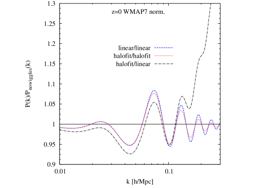
Figure 1: BAO imprint in power spectrum. To highlight the effect of the acoustic oscillations, we plot the ratio of the spectrum including the BAO wiggles to that of the corresponding power spectrum without BAO wiggles. Dashed line: ratio of linear power spectra with and without BAO. Dotted line: ratio of non-linear halofit corrected power spectra with and without BAO. Dashed-dotted line: ratio of non-linear halofit corrected power spectrum to linear “no-wiggle” spectrum. The latter highlight the effects of non-linearities.

We compare three pairs of spectra. The first pair compares the linear BAO wiggle spectrum to the corresponding linear ”no-wiggle” one. For both we use the outcome from the Eisenstein & Hu expression eqn. (10). The second pair consists of the non-linear spectrum with BAO wiggles and the corresponding non-linear one with wiggles smoothed out. Both spectra are obtained from the corresponding linear spectra, subsequently transformed via the halofit formula. The third pair compares the full non-linear, halofit corrected, spectrum with baryonic wiggles to that of the no-wiggles linear spectrum.

The first pair nicely illustrates the imprint of the baryonic acoustic oscillations. The impact of non-linearities is most starkly exemplified by the third pair, revealing a dramatic rise of the spectral amplitude at high frequencies. However, the effect of acoustic wiggles is not dramatically changed when comparing the corresponding non-linear spectrum to the non-linearly evolved ”no-wiggle” one. Its principal effects is merely a lowering of amplitude, of not more than a few percent and mainly visible at higher order harmonics.

2.5 Skewness & Non-linearities

On the basis of the power spectra in figure 1, we may expect that non-linearities will slightly affect the estimates of the skewness $S_{3}$. The lowering of the amplitude of the BAO wiggles in the non-linear regime should lead to a weakening of the BAO signal in $S_{3}$.

Figure 2 plots the skewness, computed from equations (4) and (8), for linear and non-linear power spectrum. To enhance our appreciation of the effect that the BAOs have on the result, we plot the ratio of the skewness obtained for a power spectrum with the acoustic wiggles to that of the corresponding ”no-wiggle” spectrum”. The dashed line marks the ratio of $S_{3}(R)/S_{3}^{nowiggles}(R)$ for the linear power spectra, the dotted line for the non-linear halofit-corrected spectra.

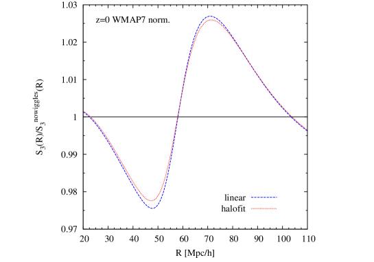
Figure 2: Reduced skewness and non-linearities. The lines depict the ratios of skewness computed using spectra including BAO wiggles to that computed with ’no-wiggles’ spectra. Dashed line: skewness following from linear power spectra. Dotted line: skewness following from non-linear halofit corrected power spectra.

The first observation is that we indeed find a clear imprint of the baryonic oscillations in the skewness $S_{3}$, in both the linear and the non-linear situation at the 2 to 3 percent level. The amplitude of the BAO signal in $S_{3}$ is slightly smaller for the non-linear situation than the linear one. Of real importance is the observation that the the non-linear evolution of the power spectrum does not lead to a shift in the scale dependence of the skewness signal. The scale at which we find the peak and the minimum in the BAO impact on $S_{3}$ remains the same. Also, there is no change in the scale at which the BAO effect changes from negative to positive. As we will discuss later, the latter will be of crucial significance.

3 Results

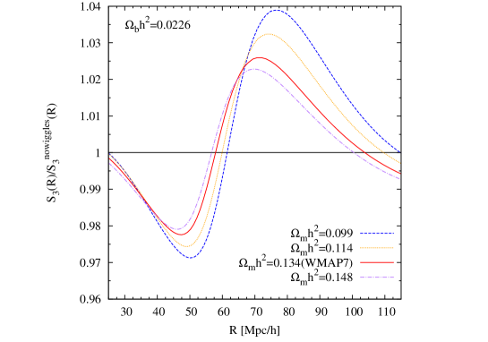
Figure 3: The acoustic oscillations imprint in the skewness $S_{3}$. In all cases we show the skewness computed using non-linear P(k) with wiggles divided by the skewness computed for ’no-wiggles’ power spectrum. The lines depict models with different values of $\Omega_{m}h^{2}$: 0.099 - the dashed line, 0.114 - the dotted line, 0.134 (WMAP7) - the solid line and 0.148 marked by dashed-dotted line. For all models the baryon density has the same value $\Omega_{b}h^{2}=0.0226$.

Having established the basic ingredients of our study, we next turn to the principal results of this study.

3.1 Baryonic Fraction

Figure 3 plots the ratio of the skewness for a spectrum with and without wiggles, $S_{3}(r)/S_{3}^{nowiggles}(r)$, for a range of LCDM cosmologies in which baryons constitute a different fraction of the non-relativistic matter content of the Universe. The baryon density is the same for all models, $\Omega_{b}h^{2}=0.0226$, a value which is tightly constrained by the CMB temperature anisotropy power-spectrum (e.g. Komatsu et al. (2011)). The total matter density varies from $\Omega_{m}h^{2}=(0.099,0.114,0.134,0.148)$.

In all cosmologies, the BAO skewness signal consists of a characteristic pattern. Starting from small scales, we observe a decrease of the skewness as the scale increases, reaching a minimum at scales of roughly $45-50h^{-1}\,{\rm Mpc}$. Subsequently, it climbs towards values larger than unity, which it reaches at a scale of $\sim 55-60h^{-1}\,{\rm Mpc}$, after which it increases towards a peak value of $2-4\%$ at a scale of around $75-80h^{-1}\,{\rm Mpc}$. Towards larger scales it gradually falls off towards unity.

We immediately observe that the BAO skewness signal increases strongly as $\Omega_{m}$ is lower and baryons constitute a more prominent fraction of matter content of the Universe. While the amplitude of the BAO skewness signal is responding systematically to the cosmic baryon fraction, it does not seem to exceed the $\sim 3-4\%$ level. In this sense, the BAO imprint is smaller that that seen in the corresponding power spectrum of density perturbations, where the wiggles may amount to a $\sim 10\%$ effect.

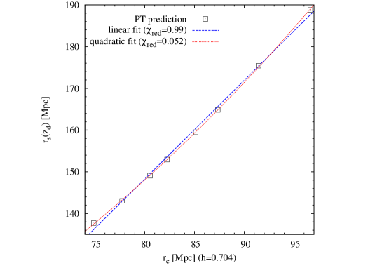
Figure 4: The dependence of the sound horizon scale ($r_{s}$) on the crossing scale ($r_{c}$). The boxes mark the values predicted by PT skewness values (see Fig. 3). Two lines show our fit to this scaling: the linear fit (the dashed line) and quadratic fit (the dotted line). The values of $r_{c}$ where rescaled to Mpc using value of $h=0.704$.

Table 1: The sound horizon scale $r_{s}$ at the baryon drag epoch $z_{d}$ and the corresponding crossing scale ion $S_{3}$ signal $r_{c}$. All models are computed with fixed $\Omega_{b}h^{2}=0.0226$. Values of $r_{c}$ are obtained with use of $h=0.704$.

$\Omega_{m}h^{2}$	$r_{s}(z_{d})$[Mpc]	$r_{c}$[Mpc]	$z_{d}$
0.099	164.82	87.24	1016.04
0.114	159.48	85.13	1018.14
0.134	152.95	82.24	1020.48
0.148	149.1	80.54	1021.67

3.2 Skewness Scale & Sound Horizon

We also make the interesting observation that the main wiggle in the skewness appears at a considerably smaller scale than that of the BAO peak in the two-point correlation function $\xi_{2}(r)$ (e.g. Crocce & Scoccimarro, 2008). This goes along with the finding that the BAO imprint on the skewness is visible over a considerable larger range of scales than that in the two-point correlation function. While for the latter, the BAO signal is noticeable on scales from roughly $80h^{-1}\,{\rm Mpc}$ to $130h^{-1}\,{\rm Mpc}$, the skewness is affected over a wider range of $20h^{-1}\,{\rm Mpc}$ to $100h^{-1}\,{\rm Mpc}$.

While the amplitude change of the skewness is closely related to the effective baryon fraction $f_{b}$ of a cosmological model, the scales associated with the wiggle should be correlated with the scale of the acoustic horizon. The scale of the acoustic horizon $r_{s}$ is a fundamental aspect of the physics of baryonic acoustic oscillations. It is the physical scale of the largest acoustic oscillations at the epoch of recombination, and as such is the scale imprinted in the BAOs visible in the distribution of galaxies and baryons in the Universe. Determining the apparent BAO scale over a wide range of redshifts, and relating it to the sound horizon, is the goal of a large number of current and future galaxy redshift surveys. (Seo & Eisenstein, 2007; Meiksin et al., 1999; Seo & Eisenstein, 2003; White, 2005).

To enable the exploitation of the information content of the skewness on the acoustic oscillations, it is therefore of fundamental importance to establish the connection of the sound horizon scale with the characteristic scales we find in the BAO feature in $S_{3}$. To this end, we compare the sound horizon scale $r_{s}$ for a range of cosmologies to the crossing scale $r_{c}$ at which the effect of BAO wiggles on the skewness reverses from negative to positive (see fig. 2 and 3). This scale is clearly a characteristic for the BAO imprint on skewness, and may be formally defined as the scale $r_{c}$ at which

$$\Delta_{S_{3}}(r_{c})\equiv{\displaystyle S_{3}(r_{c})\over\displaystyle S_{3}^{nowiggles}(r_{c})}=1\,.$$ (12)

In other words, it is the scale at which $\Delta_{S_{3}}(r)-1$ changes its sign from negative to positive. We have also checked that the $r_{c}$ scale is corresponding with the location of the inflection point of the $S_{3}$ curve near that scale.

We have measured the characteristic crossing scale for all models, and related them to the corresponding sound horizon scales and redshift of the baryon drag epoch - $z_{d}$ (Eisenstein & Hu, 1999). We list the measured values in table 1. To obtain a good understanding of the systematic relation between the two quantities, we have also evaluated their values for a few cosmological models that are currently disfavoured by observations, involving very low and very high $\Omega_{m}$ values. In figure 4 we have plotted the values of the sound horizon scale $r_{s}(z_{d})$ versus the measured characteristic skewness crossing scale $r_{c}$. The figure shows that the relation is close to linear.

In order to assess whether a higher order function would fit the relation between $r_{c}$ and $r_{s}$ better, we evaluated a first order and a second order fit,

$$r_{s} = a_{l}\cdot r_{c}+b_{l}\,\qquad\qquad\qquad\qquad\textrm{(}linear)\,,$$ (13)

$$r_{s} = a_{q}\cdot r_{c}^{2}+b_{q}\cdot r_{c}+c_{q}\,\qquad\qquad\textrm{(}quadratic)\,.$$ (14)

For the relation shown in figure 4, we have found $a_{l}=2.365$ and $b_{l}=-40.92$ for the linear fit, with $\chi^{2}_{red}=0.99$. The quadratic fit appears to be considerably better, and has a $\chi^{2}_{red}=0.052$ at parameters $a_{q}=0.0187$, $b_{q}=-0.934$ and $c_{q}=95.538$.

The important conclusion from this result is that it is indeed possible to determine the sound horizon scale at the baryon drag epoch, $r_{s}(z_{d})$, if we can succeed in successfully measuring the characteristic skewness crossing scale $r_{c}$.

3.3 Skewness BAO signature

As a final aspect of our analysis, in figure 5 we plot the behaviour of the reduced skewness as a function of (top-hat) scale $R$, at scales where the BAO feature is most prominent. The red solid line represents the skewness, as predicted by perturbation theory, for a power spectrum with BAO wiggles. For comparison we also plot the skewness resulting from the power spectrum with a ’no-wiggle’ transfer function.

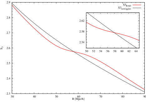
Figure 5: Skewness BAO feature. The red solid line represents the volume-averaged skewness as function of top-hat scale. It shows the characteristic skewness BAO feature, a mild shoulder around the characteristic crossing scale $r_{c}$. For comparison, the dotted line represents the skewness for a ”no-wiggle” power spectrum. The insert zooms in on the shoulder at the crossing scale $r_{c}$.

For the spectrum with wiggles, we find a characteristic shoulder at around the crossing scale. The conclusion from this comparison is that it should indeed be possible, at the $1-2\%$ level, to find the imprint of baryonic acoustic oscillations. In an idealised survey, without systematic errors and bias, it should therefore be possible to detect the BAO feature.

4 Summary and Discussion

In this report we have studied the imprint of baryonic acoustic oscillations (BAOs) on the skewness of the density field, i.e. its reduced third moment. The skewness of the density field has been found earlier to be a robust test of the gravitational instability mechanism on cosmological scale. Amongst others, it may function as a probe of the nature of gravity (e.g. Hellwing et al., 2010), and of the initial conditions itself (Durrer et al., 2000; White, 1999). This has prodded us to investigate whether the skewness could also help towards inferring cosmological relevant information via BAOs.

To investigate the question of the BAO sensitivity of skewness, we have resorted to perturbation theory. From this, we obtain an integral expression for the skewness, dependent on the power spectrum. To model the baryonic acoustic oscillations, we have used the linear power spectra expressions of Eisenstein & Hu (1998, 1999). To take account of the non-linearities in the evolving matter density field, we use the approximate analytical expressions of Smith et al. (2003).

We find that the BAO skewness signal is characteristic and may not only be detectable in the observational reality, but may even offer a potentially powerful alternative to existing means of probing BAOs. The BAO skewness signal appears to have an amplitude in the order of $3-4\%$. Interestingly, it stretches out over a substantial range of scales, from $\sim 20-100h^{-1}\,{\rm Mpc}$ and occurs at much smaller scales than the BAO imprint on power spectrum and correlation function. Perhaps most importantly, we have established a strict, near-linear relation between the sound horizon scale at the baryon drag epoch and the scale at which the BAO skewness signal crosses from negative to positive.

Even though the amplitude of the BAO skewness signal is somewhat lower than that of the BAO wiggles in the power spectrum and correlation function, it is far less sensitive to several systematic effects that still represent a major challenge for inferring cosmological parameters on the basis of BAO measurements in observational surveys. One major advantage of the BAO skewness signal over that in second order measures like the two-point correlation function and power spectrum, is that it is less sensitive to the bias of the galaxy population with respect to the mass distribution. If the galaxy density is a local function of the mass density, the relation between the skewness and the variance of the density field is preserved (Juszkiewicz et al., 1995; Fry & Gaztanaga, 1993). In other words, the shape of the $S_{3}$ reduced skewness as a function of scale is preserved when one concerns linear and local biasing of the density field. A second, and perhaps even more prominent advantage, is that the skewness - in the weakly non-linear regime - is relatively insensitive to redshift space distortions (Bouchet et al., 1992; Hivon et al., 1995; Bouchet et al., 1995).

While this short publication is meant to establish the feasibility of using skewness to probe BAOs, there are numerous issues and details that will be discussed and evaluated in an upcoming study. One major issue is the influence of non-linearities in the density field. Subtle non-linear effects may go beyond the scope of what the non-linear halofit power spectra may model. Also, the complexities of galaxy bias may only be adequately modelled by means of large N-body simulations and realistic galaxy formation models. On the other hand, the current observational estimates of $S_{3}$ from the SDSS (Ross et al., 2007) and 2dFGRS (Croton et al., 2004, 2007) are characterised by relative big errors. This suggests that detection of the BAO feature will be difficult. In the end, proper modelling of hydrodynamical and radiative processes will be essential for a truly full treatment of non-linear and biasing effects (Guillet et al., 2010).

Appendix A Derivation of the analytical form for the $\gamma_{1}(R)$

To derive expression 8 for the $\gamma_{1}$ parameter, we proceed as follows. The $\gamma_{1}$ parameter is defined as

$$\gamma_{1}\equiv-{{\textrm{d}\log\sigma^{2}(R)}\over{\textrm{d}\log R}}\,,$$ (15)

with $\sigma^{2}(R)\equiv\langle\delta^{2}(R)\rangle$ the second moment of the density contrast smoothed on (comoving) scale $R$. For a tophat filter, the latter is defined as

$$\delta_{R}(\vec{x})=\int\delta(\vec{x^{\prime}})W_{R}(|\vec{x}-\vec{x^{\prime}}|)\textrm{d}^{3}x^{\prime}\,,$$ (16)

where the expression for the tophat filter $W_{R}(x)$ is

$$W_{R}(x)\equiv\left\{\begin{array}[]{ll}{3/4\pi R^{3}}\,,\quad x\leq R\,,\\ 0,\quad\quad\quad\quad x>R\,.\end{array}\right.$$ (17)

Using the integral expression for the density contrast, we find the following integral expression for the second moment of the density field (Peebles (1980)):

$$\langle\delta_{R}^{2}(\vec{x})\rangle=$$

$$\iint\textrm{d}^{3}x^{\prime}\textrm{d}^{3}x^{\prime\prime}\langle\delta(\vec{x^{\prime}})\delta(\vec{x^{\prime\prime}})\rangle W_{R}(|\vec{x}-\vec{x^{\prime}}|)W_{R}(|\vec{x}-\vec{x^{\prime\prime}}|)$$

$$=\iint\textrm{d}^{3}x^{\prime}\textrm{d}^{3}x^{\prime\prime}\xi(\vec{x^{\prime}}-\vec{x^{\prime\prime}})W_{R}(\vec{x^{\prime}})\cdot W_{R}(\vec{x^{\prime\prime}})\,.$$ (18)

It is convenient to evaluate this integral expression in Fourier space. To this end, we use the following Fourier conventions,

$$\delta(\vec{x}) = (2\pi)^{-3/2}\int\delta_{k}e^{i\vec{k}\cdot\vec{x}}\textrm{d}^{3}k\,,$$

$$\delta_{k} = (2\pi)^{-3/2}\int\delta(\vec{x})e^{-i\vec{k}\cdot{x}}\textrm{d}^{3}x\,.$$ (19)

Recasting the double integral in equation 18 to Fourier space yields

$$\sigma^{2}(R)=(2\pi)^{-3}\iint\textrm{d}^{3}k\textrm{d}^{3}k^{\prime}\langle\delta_{k}\delta_{k^{\prime}}\rangle e^{i\vec{k}\cdot\vec{x}+i\vec{k^{\prime}}\cdot\vec{x}}W(kR)W(k^{\prime}R)\,,$$ (20)

leading to the following expression in terms of the power spectrum $P(k)$,

$$\sigma^{2}(R) = (2\pi)^{-3}\int\textrm{d}^{3}kP(k)W^{2}(kR)$$ (21)

$$= {1\over 2\pi^{2}}\int_{0}^{\infty}\textrm{d}kk^{2}P(k)W^{2}(kR)\,.$$

where the power spectrum is defined as the Fourier transform of the variance,

$$\langle\delta_{k}\delta_{k^{\prime}}\rangle=P(k)\delta_{D}(\vec{k}+\vec{k^{\prime}})\,,$$ (22)

in which $\delta_{D}$ is the Dirac delta function. The Fourier expression for the tophat filter, $W(kR)$, is given by

$$W(kR)={3\over(kR)^{3}}(\sin kR-kR\cos kR)={3\over x}j_{1}(x)\,,$$ (23)

with $j_{1}(x)$ the first order spherical Bessel function.

Differentiation of $\sigma^{2}(R)$ by $R$ yields

$${\textrm{d}\sigma^{2}_{R}\over\textrm{d}R}={\textrm{d}\sigma^{2}_{R}\over\textrm{d}R}={1\over\pi^{2}}\int_{0}^{\infty}\textrm{d}kP(k)k^{3}W(kR){\displaystyle\textrm{d}W(kR)\over\displaystyle\textrm{d}(kR)}\,,$$ (24)

where we have used the fact that

$${\textrm{d}W^{2}(kR)\over\textrm{d}R}=2kW(kR){\textrm{d}W(kR)\over\textrm{d}(kR)}\,.$$ (25)

From this, we may immediately find the expression for $\gamma_{1}$,

$$\gamma_{1} = -{{\textrm{d}\log\sigma^{2}(R)}\over{\textrm{d}\log R}}$$ (26)

$$= -{2\int_{0}^{\infty}\textrm{d}kP(k)k^{2}(kR)W(kR){\displaystyle\textrm{d}W(kR)\over\displaystyle\textrm{d}(kR)}\over\int_{0}^{\infty}\textrm{d}kP(k)k^{2}W^{2}(kR)}\,.$$

Recalling the fact that the spherical tophat filter is directly related to the first order Bessel function, $W(x)={3\over x}j_{1}(x)$, and using the derivation relations for Bessel functions, we find for the derivative of the tophat function,

$${\textrm{d}W\over\textrm{d}x}=-{3\over x^{2}}j_{1}(x)-{3\over x}j_{1}^{\prime}(x)=-{3\over x^{2}}j_{1}(x)+{1\over x}\left[j_{0}(x)-2j_{2}(x))\right]\,.$$ (27)

and inserting this relation into equation 26, after some manipulation immediately leads to the following expression,

$$\gamma_{1}(R)=2-{2\int_{0}^{\infty}\textrm{d}kP(k)j_{1}(kR)kR\left[j_{0}(kR)-2j_{2}(kR)\right]\over 3\int_{0}^{\infty}\textrm{d}kP(k)j_{1}^{2}(kR)}\,.$$ (28)

This relation for $\gamma_{1}$ is the central expression of this paper.

References

- Angulo et al. (2008) Angulo R. E., Baugh C. M., Frenk C. S., Lacey C. G., 2008, MNRAS, 383, 755
- Baugh et al. (1995) Baugh C. M., Gaztanaga E., Efstathiou G., 1995, MNRAS, 274, 1049
- Bernardeau (1994a) Bernardeau F., 1994a, ApJ, 433, 1
- Bernardeau (1994b) Bernardeau F., 1994b, A&A, 291, 697
- Blake & Glazebrook (2003) Blake C., Glazebrook K., 2003, ApJ, 594, 665
- Bouchet et al. (1995) Bouchet F. R., Colombi S., Hivon E., Juszkiewicz R., 1995, A&A, 296, 575
- Bouchet et al. (1992) Bouchet F. R., Juszkiewicz R., Colombi S., Pellat R., 1992, ApJ, 394, L5
- Cole et al. (2005) Cole S. et al., 2005, MNRAS, 362, 505
- Cooray et al. (2001) Cooray A., Hu W., Huterer D., Joffre M., 2001, ApJ, 557, L7
- Crocce & Scoccimarro (2008) Crocce M., Scoccimarro R., 2008, Phys. Rev. D, 77, 023533
- Croton et al. (2004) Croton D. J. et al., 2004, MNRAS, 352, 1232
- Croton et al. (2007) Croton D. J., Norberg P., Gaztañaga E., Baugh C. M., 2007, MNRAS, 379, 1562
- Drinkwater et al. (2010) Drinkwater M. J. et al., 2010, MNRAS, 401, 1429
- Durrer et al. (2000) Durrer R., Juszkiewicz R., Kunz M., Uzan J., 2000, Phys. Rev. D, 62, 021301
- Eisenstein & Hu (1998) Eisenstein D. J., Hu W., 1998, ApJ, 496, 605
- Eisenstein & Hu (1999) Eisenstein D. J., Hu W., 1999, ApJ, 511, 5
- Eisenstein et al. (1998) Eisenstein D. J., Hu W., Tegmark M., 1998, ApJ, 504, L57+
- Eisenstein et al. (2005) Eisenstein D. J. et al., 2005, ApJ, 633, 560
- Frieman et al. (2008) Frieman J. A., Turner M. S., Huterer D., 2008, ARA&A, 46, 385
- Fry & Gaztanaga (1993) Fry J. N., Gaztanaga E., 1993, ApJ, 413, 447
- Gaztañaga et al. (2009) Gaztañaga E., Cabré A., Castander F., Crocce M., Fosalba P., 2009, MNRAS, 399, 801
- Guillet et al. (2010) Guillet T., Teyssier R., Colombi S., 2010, MNRAS, 405, 525
- Guzik et al. (2007) Guzik J., Bernstein G., Smith R. E., 2007, MNRAS, 375, 1329
- Hellwing et al. (2010) Hellwing W. A., Juszkiewicz R., van de Weygaert R., 2010, Phys. Rev. D, 82, 103536
- Hivon et al. (1995) Hivon E., Bouchet F. R., Colombi S., Juszkiewicz R., 1995, A&A, 298, 643
- Hu & Haiman (2003) Hu W., Haiman Z., 2003, Phys. Rev. D, 68, 063004
- Hütsi (2006) Hütsi G., 2006, A&A, 449, 891
- Juszkiewicz et al. (1993) Juszkiewicz R., Bouchet F. R., Colombi S., 1993, ApJ, 412, L9
- Juszkiewicz et al. (1995) Juszkiewicz R., Weinberg D. H., Amsterdamski P., Chodorowski M., Bouchet F., 1995, ApJ, 442, 39
- Komatsu et al. (2011) Komatsu E. et al., 2011, ApJS, 192, 18
- Laureijs et al. (2011) Laureijs R. et al., 2011, ArXiv e-prints
- Meiksin et al. (1999) Meiksin A., White M., Peacock J. A., 1999, MNRAS, 304, 851
- Padmanabhan et al. (2007) Padmanabhan N. et al., 2007, MNRAS, 378, 852
- Peebles (1980) Peebles P. J. E., 1980, The large-scale structure of the universe. Research supported by the National Science Foundation. Princeton, N.J., Princeton University Press, 1980. 435 p.
- Peebles & Yu (1970) Peebles P. J. E., Yu J. T., 1970, ApJ, 162, 815
- Percival et al. (2007) Percival W. J. et al., 2007, ApJ, 657, 51
- Perlmutter et al. (1999) Perlmutter S., Aldering G., Goldhaber G., Knop R. A., Nugent P., et al., 1999, ApJ, 517, 565
- Riess et al. (1998) Riess A. G. et al., 1998, AJ, 116, 1009
- Ross et al. (2007) Ross A. J., Brunner R. J., Myers A. D., 2007, ApJ, 665, 67
- Ross et al. (2010) Ross N. et al., 2010, in Bulletin of the American Astronomical Society, Vol. 42, American Astronomical Society Meeting Abstracts 215, p. 471.04
- Sefusatti et al. (2006) Sefusatti E., Crocce M., Pueblas S., Scoccimarro R., 2006, Phys. Rev. D, 74, 023522
- Seo & Eisenstein (2003) Seo H.-J., Eisenstein D. J., 2003, ApJ, 598, 720
- Seo & Eisenstein (2007) Seo H.-J., Eisenstein D. J., 2007, ApJ, 665, 14
- Smith et al. (2003) Smith R. E. et al., 2003, MNRAS, 341, 1311
- Smith et al. (2007) Smith R. E., Scoccimarro R., Sheth R. K., 2007, Phys. Rev. D, 75, 063512
- Sunyaev & Zeldovich (1970) Sunyaev R. A., Zeldovich Y. B., 1970, Ap&SS, 7, 3
- Szapudi et al. (1999) Szapudi I., Quinn T., Stadel J., Lake G., 1999, ApJ, 517, 54
- Tegmark et al. (2006) Tegmark M. et al., 2006, Phys. Rev. D, 74, 123507
- White (1999) White M., 1999, MNRAS, 310, 511
- White (2005) White M., 2005, Astroparticle Physics, 24, 334
- Zhan & Knox (2006) Zhan H., Knox L., 2006, ApJ, 644, 663