Non-adiabatic effects within a single thermally-averaged potential energy surface: Thermal expansion and reaction rates of small molecules

Abstract

At non-zero temperature and when a system has low-lying excited electronic states, the ground-state Born–Oppenheimer approximation breaks down and the low-lying electronic states are involved in any chemical process. In this work, we use a temperature-dependent effective potential for the nuclei which can accomodate the influence of an arbitrary number of electronic states in a simple way, while at the same time producing the correct Boltzmann equibrium distribution for the electronic part. With the help of this effective potential, we show that thermally-activated low-lying electronic states can have a significant effect in molecular properties for which electronic excitations are oftentimes ignored. We study the thermal expansion of the Manganese dimer, Mn₂, where we find that the average bond length experiences a change larger than the present experimental accuracy upon the inclusion of the excited states into the picture. We also show that, when these states are taken into account, reaction rate constants are modified. In particular, we study the opening of the ozone molecule, O₃, and show that in this case the rate is modified as much as a 20% with respect to the ground-state Born–Oppenheimer prediction.

I Introduction

In the ab initio study of the behaviour of molecular systems, it is common to perform the Born–Oppenheimer separation of the nuclear and electronic parts of the molecular wavefunction. This approximation is based in the large difference between the masses of the electrons and the nuclei,Born and Oppenheimer (1927); Echenique and Alonso (2007) and therefore becomes exact only in the classical limit for the nuclei. Computing the electronic energy spectrum for different positions of the nuclei, one obtains the different so-called Potential Energy Surfaces (PESs) —one for the electronic ground state, and one for each excited state. Now the question arises, how may we use these PESs in order to produce accurate and convenient physical models? The simplest option is ground-state Born–Oppenheimer (gsBO), or typically just Born–Oppenheimer (BO). One may then consider the nuclei to be quantum particles and solve their corresponding Schrödinger equation, or take the classical limit and perform BO Molecular Dynamics. In any case, a model based on only one PES (usually the ground state one) is an adiabatic approximation, based on the neglect of the non-adiabatic couplings.

However, at non-zero temperature and when a system has low-lying excited electronic states, these electronic states are involved in any chemical process, and their influence produces the so-called non-adiabatic effects. In this paper, we use a thermodynamically accurate generalization, introduced in Ref. Alonso et al., 2010, of the gsBO potential, built with the PESs of the lowest-lying electronic states appropriately weighted to produce the correct Boltzmann equilibrium distribution of the electronic part, to specifically study the thermal expansion and reaction rates of small molecules. For both phenomena, a substantial amount or research is constructed on the implicit assumption of one electronic potential, which may be fitted to experimental results or computed ab initio. The possibility of electronic excitations is typically either ignored or handled by independently considering each of the excited PES (although we can mention Ref. Mazzola et al., 2012 as a very recent exception to this general trend, with similar aims to the ones we pursue here). The thermally averaged potential energy surface that we use in this work permits to include electronic excitations while still preserving the single potential methodology.

The possibility, in which our formalism is based, of dividing a system of particles into a quantum and a classical subsystem (typically, electrons and nuclei) is of wide interest in several areas of physics and chemistry. If the temperature is of the order of the electronic gap or larger and excited electronic energy levels have to be included in the formalism, a variety of approaches can be considered.Zhu et al. (2005); Truhlar (2007); Schmidt et al. (2008); Worth and Ceberbaum (2004); J. Martinez et al. (1996); Nakamura (2002); Baer (2006); Prezhdo (1999) For example, the decay-of-mixing method by Truhlar and coworkers Zhu et al. (2005); Truhlar (2007) constitutes a powerful mixed quantum-classical scheme for modeling non-Born-Oppenheimer chemistry, although the incorporation of temperature to these methods has not been studied as far as we are aware. In the case of Ehrenfest dynamics, which also includes non-adiabatic effects at a different level, the temperature has been introduced through the formulation of Nosé.Alonso et al. (2011); [ItisalsoworthremarkingthatsomecommoncriticismsthatstatedthatEhrenfestisafullycoherentmethod; andthusitcannotaccountforsuchimportanteffectsasmixinganddecoherence; haverecentlybeenchallenged:]Alonso2012

The temperature dependence of molecular properties (geometry and vibrational frequencies) of free molecules has been a subject of research for more than 60 years,Bartell (1955) with new theoretical analyses coming out still in very recent times.Varga et al. (2010, 2011) From the experimental viewpoint, on the other hand, several studies of hot molecules (Bartell, 1979; Bartell et al., 1979; Goates and Bartell, 1982, 1982; Bartell et al., 1984) have found thermal expansion of bond lengths. In this paper we calculate the temperature dependence of the bond length in the case of diatomic molecules in which nuclei can be treated as classical particles. Although bond-length expansion as the temperature increases is expected even for temperature-independent potentials such as the gsBO one, the use of our thermodynamically more accurate effective potential adds new non-adiabatic effects which, as we will show for the Mn₂ dimer, may significantly alter the final quantitative results if low-lying excited states are present. These effects must be considered when performing the necessary rovibrational averaging in order to compare accurate theoretical and experimental results.

The temperature dependence of the transition rate is also a constant subject of study Hänggi et al. (1990); Fleming et al. (2011); Bothma et al. (2010) and, more recently, the question has been asked of whether or not quantum tunneling below the energy barrier significantly enhances the reaction rate.Fleming et al. (2011); Bothma et al. (2010); Iyengar et al. (2008) Using a general framework to describe tunneling,Bothma et al. (2010) it is shown that tunneling below the barrier only occurs for temperatures less than a reference one, denoted by $T_{0}$, and which is determined by the curvature of the ground-state PES (gsPES) at the top of the barrier. However, at non-zero temperatures and when a system has low-lying excited electronic states, all estimates based on the ground-state PES should be reconsidered.

As demonstrated in this work using our thermodynamically accurate generalization of the gsBO potential, the inclusion of low-lying electronic states into the picture may significantly alter the reaction rates and the curvature near the top of the barrier. As a model system to exemplify the added effects, we have chosen the transition between the open and closed forms of the ozone molecule, in which the barrier lies in a region where there is an avoided crossing between the ground and first-excited electronic states. Having no problems whatsoever with avoided-crossing situations, our effective potential is a convenient choice to account for the influence of low-lying excited states in this phenomenon at non-zero temperature.

In Sec. II, we provide a comprehensive summary of the definition and meaning of the effective potential introduced in Ref. Alonso et al., 2010 which includes the effect of excited electronic states and which will be used throughout the document. In Sec. III.1, we present the first application of the effective-potential technique: the study of the thermal expansion of the Manganese dimer, Mn₂; in Sec. III.2, we discuss the influence of the inclusion of low-lying excited electronic states on the reaction rate of small molecules. Reaction rates are affected on the one hand by the energy barrier reduction. On the other hand, the curvature at the top of the barrier is smaller for our effective potential than for the gsPES. In this section we will also study the case of the opening of the ozone molecule, O₃. Finally, in Sec. IV, we comment on the most important conclusions of this work and highlight some possible implications and future lines of research.

II Theoretical framework

Let us have a quantum-classical system formed by $N$ classical particles described by their Euclidean coordinates $R:=(\vec{R}_{1},\ldots,\vec{R}_{N})$ and momenta $P:=(\vec{P}_{1},\ldots,\vec{P}_{N})$, and $n$ quantum particles described by an $n$-body wavefunction $|\psi\rangle$. The starting point of our formalism is the assumption that the following is an accurate formula to compute canonical equilibrium expected values of quantum-classical observables $\hat{O}(R,P)$:

$$\langle\hat{O}(R,P)\rangle=\frac{\displaystyle\int dRdP\,\mathrm{tr}\left(\hat{O}(R,P)\,e^{-\frac{\hat{H}(R,P)}{k_{\rm B}T}}\right)}{\displaystyle\int dRdP\,\mathrm{tr}\left(e^{-\frac{\hat{H}(R,P)}{k_{\rm B}T}}\right)}\,,$$ (1)

where $k_{\rm B}$ is the Boltzmann constant and $T$ the temperature, $dRdP$ denotes integration over all position and momenta in the appropriate ranges. The object $\hat{H}(R,P)$ is the quantum-classical Hamiltonian, which, in the case of molecular systems, takes the form

$$\hat{H}(R,P):=\hat{1}\sum_{K=1}^{N}\frac{\vec{P}_{K}^{2}}{2M_{K}}+\hat{H}_{e}(R)\,,$$ (2)

where $\hat{1}$ denotes the identity matrix, $M_{K}$ is the mass of the $K$-th nucleus, and the electronic Hamiltonian, $\hat{H}_{e}(R)$, contains all particle interactions and the electronic kinetic term (see Ref. Echenique and Alonso, 2007 for an explicit expression).

It is also convenient to write Eq. (1) as

$$\langle\hat{O}(R,P)\rangle=\int dRdP\,\mathrm{tr}\left(\hat{O}(R,P)\hat{\rho}_{\mathrm{eq}}(R,P)\right)\,,$$ (3)

in terms of a $(R,P)$-dependent equilibrium density matrix, defined by

$$\hat{\rho}_{\mathrm{eq}}(R,P):=\frac{\displaystyle e^{-\frac{\hat{H}(R,P)}{k_{\rm B}T}}}{\displaystyle\int dR^{\prime}dP^{\prime}\,\mathrm{tr}\left(e^{-\frac{\hat{H}(R^{\prime},P^{\prime})}{k_{\rm B}T}}\right)}\,.$$ (4)

As shown in Ref. Alonso et al., 2010, the justification of Eq. (1) for computing equilibrium expected values in quantum-classical models stems on the one hand from plausibility arguments related to the classical limit of the behaviour of the nuclei, such as the ones given in Ref. Mauri et al., 1993. However, it can also be obtained as the zero-th order approximation (in the quantum-classical mass ratio) to the canonical equilibrium associated with an, in principle, more rigorous quantum-classical formulation based on the Wigner formalism, as shown by Kapral and Ciccotti Kapral and Ciccotti (1999) and Nielsen et al. Nielsen et al. (2001). It may also be rationalized by entropic argumentsent . In any case, and as it can be seen in the references in Ref. Alonso et al., 2010, irrespective of how good an approximation Eq. (1) is for any given application —always a difficult question—, it is often the desired, target expectation value when designing quantum-classical schemes.

The main realization in which the effective potential that we will use in this work is based is that, for observables which do not depend explicitly on the electronic degrees of freedom, i.e., which are of the form

$$\hat{O}(R,P)=\hat{1}\,O(R,P)\,,$$ (5)

where $O(R,P)$ is a number, the target expected value in Eq. (1) can be rewritten as

$$\langle O(R,P)\rangle=\frac{\displaystyle\int dRdP\,O(R,P)\,e^{-\frac{H_{\mathrm{eff}}(R,P;T)}{k_{\rm B}T}}}{\displaystyle\int dRdP\,e^{-\frac{H_{\mathrm{eff}}(R,P;T)}{k_{\rm B}T}}}\,.$$ (6)

Now, $H_{\mathrm{eff}}(R,P;T)$ is a purely classical, $T$-dependent, effective Hamiltonian defined as

$$H_{\mathrm{eff}}(R,P;T) := -k_{\rm B}T\,\mathrm{ln}\,\mathrm{tr}\,e^{-\frac{\hat{H}(R,P)}{k_{\rm B}T}}$$ (7)

$$= \sum_{K=1}^{N}\frac{\vec{P}_{K}^{2}}{2M_{K}}-k_{\rm B}T\,\mathrm{ln}\,\mathrm{tr}\,e^{-\frac{\hat{H}_{e}(R)}{k_{\rm B}T}}$$

$$=: \sum_{K=1}^{N}\frac{\vec{P}_{K}^{2}}{2M_{K}}+V_{\mathrm{eff}}(R;T)\,,$$

where we have used Eq. (2). In the last line, we have finally defined the promised, purely classical, $T$-dependent, $P$-independent, effective potential

$$V_{\mathrm{eff}}(R;T):=-k_{\rm B}T\,\mathrm{ln}\,\mathrm{tr}\,e^{-\frac{\hat{H}_{e}(R)}{k_{\rm B}T}}\,,$$ (8)

which can be used to describe the behaviour of the nuclei in a classical mechanical setting, producing the correct target equilibrium in Eq. (1) for classical observables —by construction—, and including the influence of all the electronic excited states.

Indeed, if we consider the adiabatic basis $\{|\psi_{k}(R)\rangle\}$, which diagonalizes the electronic Hamiltonian $\hat{H}_{e}(R)$ for each fixed position of the nuclei,

$$\hat{H}_{e}(R)|\psi_{k}(R)\rangle=E_{k}(R)|\psi_{k}(R)\rangle\,,$$ (9)

being $\{E_{k}(R)\}$ the corresponding PESs, i.e., the eigenvalues of the electronic Hamiltonian as a function of the nuclear positions, then we can rewrite the effective potential in Eq. (8) as

$$V_{\mathrm{eff}}(R;T) = -k_{\rm B}T\,\mathrm{ln}\sum_{k}e^{-\frac{E_{k}(R)}{k_{\rm B}T}}$$

$$= E_{0}(R)-k_{\rm B}T\,\mathrm{ln}\left[1+\sum_{k>0}e^{-\frac{\Delta E_{k0}(R)}{k_{\rm B}T}}\right]\,,$$

where we have defined

$$\Delta E_{k0}(R):=E_{k}(R)-E_{0}(R)\,.$$ (11)

The expression in Eq. (II) explicitly shows the difference between the ground state PES, $E_{0}(R)$, i.e., the gsBO potential, and the effective potential $V_{\mathrm{eff}}(R;T)$ introduced in Ref. Alonso et al., 2010 and used in this work. In particular, it is worth remarking that

• At $T=0$, our effective potential becomes the gsBO one. Indeed, it is easy to see from Eq. (II) that

  $$\lim_{T\to 0}V_{\mathrm{eff}}(R;T)=E_{0}(R)\ ,\quad\forall R\,.$$ (12)

• The same reasons that produce the previous result allow us to include in the sum in Eq. (II) only the lowest-lying electronic states and still get a good enough approximation to the exact expression if the temperature is low compared to the states we are neglecting, i.e., if $k_{\rm B}T\ll\Delta E_{k0}(R)$ for them. This fact will be used in the practical cases presented in the next sections.

• It can be seen from Eq. (II) that an exact property of the effective potential is that it is strictly lower than the gsPES, i.e., $V_{\mathrm{eff}}(R;T)\leq E_{0}(R)$, $\forall R,T$. However, since an additive constant in a potential energy is not measurable, it must be noticed that this inequality is relevant only inasmuch the difference $E_{0}(R)-V_{\mathrm{eff}}(R;T)$ actually depends on $R$. See Secs. III.1 and III.2 for concrete examples of this situation.

• As we discussed in Ref. Alonso et al., 2010, from Eq. (II), we see that, if the second derivative of $\Delta E_{10}$ at a barrier top $q_{B}$ verifies

  $$\frac{\partial^{2}\Delta E_{10}}{\partial q^{2}}(q_{B})\left(1+e^{\frac{\Delta E_{10}(q_{B})}{k_{\rm B}T}}\right)>\frac{1}{k_{\rm B}T}\left(\frac{\partial\Delta E_{10}}{\partial q}(q_{B})\right)^{2}\,,$$ (13)

  then we can prove

  $$\left|\frac{\partial^{2}V_{\rm eff}}{\partial q^{2}}(q_{B};T)\right|<\left|\frac{\partial^{2}E_{0}}{\partial q^{2}}(q_{B})\right|\,,$$ (14)

  i.e., the curvature of the effective potential at the barrier top is smaller than the one associated to the gsPES. In avoided crossings —a very interesting general case, and the one actually studied in Sec. III.2— since the first excited state approaches the gsPES and then recedes from it, we have that the derivative $(\partial\Delta E_{10}/\partial q)(q_{B})$ will be approximately zero and the condition in Eq. (13) will be approximately satisfied, together with Eq. (14).

Note that in order to obtain the effective potential, and the corresponding averages, it is not necessary to compute the non-adiabatic couplings. This is a consequence of the fact that the purpose of the effective potential is the computation of averages at canonical thermal equilibrium, and not the dynamics that may lead to it. The non-adiabatic couplings are necessary to carry the system to equilibrium – by providing the necessary channels to couple the various electronic states. Because of this, we are considering that the difference between these averages and the ones that would be obtained by considering the gsPES only is a non-adiabatic effect. However, the equilibrium averages predicted by Eq. (1) can be obtained without explicit consideration of the couplings. The magnitude of those couplings might be very relevant to compute the speed of the thermalization: small couplings may necessitate long thermalization times, but those analysis are beyond the scope of the present work.

In this respect, also note that all excited electronic states are included in the definition of the effective potential – because all states are included in Boltzmann’s equilibrium formula, regardless of how they may be coupled by external fields or, in the quantum-classical case, by the non-adiabatic couplings. The weight of each state is entirely determined by its energy. Any state is present in the averaging, even if its couplings to the ground state and to any other accessible state is zero. This is an example of ergodic difficulties, and obviously, a dynamical averaging would not include such a state unless it is already included in the initial state sampling.

The straightforward application of our scheme would then be inadequate if one is interested in computing a “restricted equilibrium” average, in which a state (or full subspace of states) is known to be absent, due to symmetry rules. The “experimental average” would not contain those states, even if the true canonical ensemble average does. However in this situation it would be easy to correct our scheme by simply not including the forbidden states in the formulas.

III Results

III.1 Non-adiabatic effects on the thermal expansion of the Mn₂ dimer

Theoreticians usually identify the “molecular structure” with the equilibrium structure, i.e., the point determined by the absolute minimum of the ground state Born-Oppenheimer potential energy surface (gsPES). This point in $\mathbb{R}^{3N}$ space ($N$ being the number of atoms) is well defined and has an easy intuitive meaning: the position occupied by the nuclei at equilibrium, if they had infinite mass (in which case they would be classical point particles). This geometry corresponds to a motionless molecule, that does not exist because molecules vibrate and move even at zero temperature. Therefore, this equilibrium structure is a theoretical concept that is not provided —at least not directly— by the experimental techniques utilized to probe molecular structure.

In fact, different experimental techniques yield different averaged results, whose value and meaning depend on the physical process involved in the measurement. For example, X-ray diffraction provides distances between the electronic charge distribution centroids. Gas-phase electron diffraction (ED), on the other hand, provides internuclear distances. Microwave spectroscopy measures moments of inertia, which can be directly related to nuclear distances to the molecular center of mass. Infrared, Raman, and ultraviolet spectroscopies can also be used for complementary analysis. In all cases, the results are averaged over the populated rotational and vibrational molecular states —and, as we will show below, possibly over different electronic potential energy surfaces. Those techniques achieve a remarkable precision (of the order of 0.001 Å), but nevertheless provide different numbers each one of them.

Figure 1: Six lowest lying PESs of the Mn₂ dimer, taken from Ref. [Tzeli et al., 2008]. The calculations were performed through multireference variational calculations coupled with augmented quadruple correlation consistent basis sets. These PESs correspond to the ground state “manifold”, that correlates to ground state Mn atoms.

In order to compare the results obtained in different experiments and in precise ab initio calculations, it is necessary to use a “common denominator” representation, which can very well be the equilibrium structure mentioned above, usually called the r_e structure. One must therefore know how to relate the experimental result to this concept. In an ED experiment at a given temperature, for example, one obtains the so-called r_a structure, an operational concept with no clear physical meaning. It can be related, however, to the thermally averaged internuclear distance, or r_g structure, which is of physical significance. It is not equivalent to the $r_{e}$ structure, not even at 0 K, because of the vibrational and rotational (also called centrifugal) distortions. The relationship between $r_{e}$ and an averaged structure such as $r_{g}$ is not straightforward, but must be considered if we want to validate high precision theoretical ab initio calculations with experimental results or vice versa. This relationship was first considered by Bartell,Bartell (1955) and has later been developed by several authors.Kuchitsu and Bartell (1962, 1961); Toyama et al. (1964); Herschbach and Laurie (1962); Spiridonov et al. (2001); Butayev et al. (1985) It was soon realized that, in general, molecules expand as temperature increases, due to both the anharmonicity of the vibrations and to the centrifugal “force” that rotations exert on the structure.

In all these studies, an assumption is implicitly made: the electrons are adiabatically tied to their ground state, and therefore the analysis is performed by considering the gsPES only. However, as discussed in the introduction, the existence of non-zero non-adiabatic couplings permits the system to visit electronic excited states, and the thermodynamic averaging should account for this possibility if the energy gap between the gsPES and the excited ones is not large in comparison with the thermal energy, $k_{\rm B}T$. If calculations and experiments are to be succesfully compared, it is therefore necessary to consider the possible effect of the excited electronic states. We propose the use of our thermally averaged potential energy surface introduced in the previous section for this purpose.

In principle, the rotational-vibrational averaging necessary to compute $r_{g}$ must be performed assuming quantum-mechanical nuclei. This is obvious at 0 K, where the zero-point vibration would be completely absent in a classical treatment. However, we are mostly interested in the high-temperature regime —where the excited electronic states are expected to play a larger role and the system becomes classical. This fact can be exemplified by looking at closed —albeit approximate— theoretical formulae that exist for the simplest cases on which we concentrate in this study: diatomic molecules. By truncating the Taylor expansion of the PES around the equilibrium bond length, i.e.:

$$V(r)=\frac{1}{2}k_{2}(r-r_{e})^{2}-k_{3}(r-r_{e})^{3}\,,$$ (15)

Toyama et al. Toyama et al. (1964) computed, in the quantum case, the temperature-induced variation of the average internuclear distance (with respect to $r_{e}$) as:

$$\langle\Delta r\rangle(T) := \langle r\rangle(T)-r_{e}$$ (16)

$$= \frac{2k_{\rm B}T}{k_{2}r_{e}}+\frac{3k_{3}\omega_{e}}{2k_{2}^{2}}\coth\left[\frac{\omega_{e}}{2k_{\rm B}T}\right]\,,$$

where $\omega_{e}$ is the vibrational frequency at equilibrium ($\omega_{e}=\sqrt{k_{2}/\mu}$, where $\mu$ is the reduced mass of the two nuclei).

The first term in Eq. (16) is the centrifugal distortion; it arises from the harmonic potential term in Eq. (15), and can be considered as the variation in the average bond length caused by the overall molecular rotations. Interestingly, a classical treatment leads to the same expression for this term. The second term, on the contrary, has a genuinely quantum behaviour at low temperatures. In fact, it does not approach zero as $T\to 0$ K, producing a zero-point vibration variation of the bond length with respect to $r_{e}$. We can now take the classical limit by considering $\mu\to\infty$, in which case this second term becomes linear in $T$: $3k_{3}k_{\rm B}T/k_{2}^{2}$. But note that the same behaviour occurs if we take $k_{\rm B}T$ large with respect to $\omega_{e}$ —i.e., the system becomes classical for large enough temperatures.

In view of this, and since we are interested in the high-temperature regime in which our effective potential may significantly differ from the gsPES, we have used the classical approximation to compute the average bond length. To this end, we used Eq. (6), which for the dimer case (and considering that the function $O(R,P)$ is in this case nothing else than the internuclear distance $r=|\vec{R}_{1}-\vec{R}_{2}|$), reads:

$$\langle r\rangle_{\rm eff}(T)=\frac{\int_{0}^{L}\!{\rm d}r\;r^{3}e^{-\frac{V_{\rm eff}(r;T)}{k_{\rm B}T}}}{\int_{0}^{L}\!{\rm d}r\;r^{2}e^{-\frac{V_{\rm eff}(r;T)}{k_{\rm B}T}}}\,.$$ (17)

Note the presence of a somewhat arbitrary upper limit of integration $L$. This value cannot be made arbitrarily large, since in the limit $L\to\infty$, the equilibrium bond length is also infinite (assuming that, as it is always the case, the potential function remains finite at large internuclear distances). In fact, at equilibrium and at any non-zero temperature, a dilute gas of diatomic molecules in an infinite space does not really contain dimers but isolated atoms. In the real world, dimers exist because there is always some form of container, or they are in a very long-lived metastable state. In practice, one must choose a value of $L$ such that the results are almost insensitive to small variations of it —acknowledging that, if $L$ is increased to very large values, the value of $\langle r\rangle(T)$ will start growing.

The question that we want to answer here is whether or not the use of the effective potential in Eq. (17) leads to significantly different results with respect to the results obtained using only the gsPES, i.e.:

$$\langle r\rangle_{0}(T)=\frac{\int_{0}^{L}\!{\rm d}r\;r^{3}e^{-\frac{E_{0}(r)}{k_{\rm B}T}}}{\int_{0}^{L}\!{\rm d}r\;r^{2}e^{-\frac{E_{0}(r)}{k_{\rm B}T}}}\,.$$ (18)

The answer cannot of course be universal, and depends on the chosen system and the temperature regime observed. In order to illustrate the issue, we have concentrated on the Mn₂ molecule; a Van der Waals weakly-bound molecule and a specially difficult theoretical case,Wang and Chen (2004); Yamamoto et al. (2006); Tzeli et al. (2008) for which a good feedback between experiments and theory could help validate the conflicting theoretical results. As we shall show, the existence of very low-lying excited electronic states in the vicinity of the equilibrium distance has an important effect on $\langle r\rangle(T)$, and therefore it is crucial to consider them to make proper comparisons.

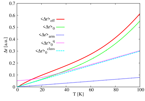
Figure 2: Calculated variation of the average internuclear distance as a function of temperature for Mn₂. $\langle\Delta r\rangle_{\rm eff}$ is the result computed using, in Eq. 17, the effective potential including all six lowest-lying states in Fig. 1, while $\langle\Delta r\rangle_{0}$ is only computed with the gsPES. $\langle\Delta r\rangle_{0}^{q}$ is the third-order approximation to the quantum result, as calculated using Eq. (16), and $\langle\Delta r\rangle_{0}^{\rm class}$ is its classical limit. $\langle\Delta r\rangle_{\rm arm}$ is the centrifugal term, common to all cases.

To build our averaged potential defined in Eq. II, we depart from the potential energy curves provided by Tzeli et al. Tzeli et al. (2008), computed from first principles with very accurate multireference variational calculations. We only consider the six almost-degenerate, lowest-lying states, displayed in Fig. 1. We have adjusted these curves to Morse functions, i.e.:

$$V(r)=D\left[e^{-2\alpha\frac{r-r_{e}}{r_{e}}}-2e^{-\alpha\frac{r-r_{e}}{r_{e}}}\right]+V_{\infty}\,.$$ (19)

By finding the best match for the parameters $D,\alpha,r_{e}$ and $V_{\infty}$, an almost perfect fit can be obtained with respect to the results of Tzeli et al. The plot clearly shows the reasons for choosing Mn₂ in this study: the lowest-lying states are extremely close to each other, and the potential well is very shallow.

The results are shown in Fig. 2. The two key curves are the ones denoted by $\langle\Delta r\rangle_{\rm eff}$ and $\langle\Delta r\rangle_{0}$, which are the results obtained with Eqs. (17) and (18), respectively. The difference due to the use of the effective potential instead of the ground state one is notable. It is larger than the resolution of modern experimental techniques, even in the lower-temperature range. One may then conclude that any assessment of the quality of a theoretical model based on a comparison to experimental results should consider the influence of these low-lying electronic excited states.

In Fig. 2, we also display the approximate quantum result given by Eq. (16), and denoted by $\langle\Delta r\rangle_{0}^{q}$. This quantum curve is only valid at low temperatures, since it stems from a perturbative truncation of the potential. We display it in order to demonstrate how the system behaves almost classically in most of the temperature range of the plot, thus justifying our classical treatment. Indeed, if we plot the classical limit ($\mu\to\infty$) of Eq. (16), denoted by $\langle\Delta r\rangle_{0}^{\rm class}$, it quickly becomes almost identical to $\langle\Delta r\rangle_{0}^{q}$. In this temperature region, our classical calculation, which does not truncate the potential curve, should be almost exact. Finally, for completeness, the curve $\langle\Delta r\rangle_{\rm arm}$ is the centrifugal term —the difference with the rest of the curves would be the vibrational contribution in each case.

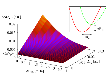
Figure 3: Variation of the average internuclear distance, at 300 K, for a fictitious dimer with two relevant PES, as schematically shown in the inset. The results are given as a function of the displacement of the excited PES with respect to the gsPES, in two directions: variation of the energy minimum $\Delta E_{10}$, and difference in the position of this minimum, $\Delta r_{e}$.

Beyond this particular example, a more general question has to be addressed when must one expect the electronic excited states to influence the thermally averaged internuclear distances —and therefore any experimental measurement of molecular geometry? A simple visual inspection of a few lowest lying excited PES, and a simple calculation with our thermally averaged PES should give us a quick answer. Two key parameters should be carefully examined: the “gap”, or difference between the gsPES and the closest excited ones, and how much the position of the minima of the two curves differ. This fact is illustrated in Fig. 3, where we have considered a fictitious dimer with two closely lying PES. The parameters of the gsPES correspond to the Hydrogen molecule, whereas the first excited PES is a rigid displacement in two directions: varying the minimum energy ($\Delta E_{10}$), and the position of the corresponding minimum ($\Delta r_{e}$).

The 2D plot displays in Fig. 3 $\langle\Delta r\rangle_{\rm eff}$ at room temperature (300 K). As the gap becomes large, the results converge towards $\langle\Delta r\rangle_{0}$, the thermal expansion entirely due to the gsPES. The plot shows how, for the results to differ significantly, the gap should not be larger than a few mHa —which is easily understood since, at 300 K, $k_{\rm B}T$ is approximately 1 mHa. But also note that, even if the gap is small, there is no change with respect to $\langle\Delta r\rangle_{0}$ if the positions of the minimum of the two curves do not differ ($\Delta r_{e}$ is small). In other words, if the two PES are merely a rigid vertical shift of each other, the thermally averaged PES is also a rigid vertical shift and nothing change.

III.2 Non-adiabatic effects on the reaction rate and the opening of ozone

Reaction-rate theory focuses on studying the behavior at long times of systems with different equilibrium states. This is a subject of great interest in many biological, chemical and physical problems. As noted by Arrhenius in 1889, Arrhenius (1889) the cornerstone of the theory is the $e^{-A/T}$ temperature dependence of the reaction rates. Such dependence can be understood in the framework of a transition-state theory where the system evolves as a function of a given reaction coordinate $q$ from the metastable state $A$ to the metastable state $C$ through an energy barrier $B$, being the activation constant related with the barrier energy $U=E_{B}-E_{A}$ (see Fig. 4).

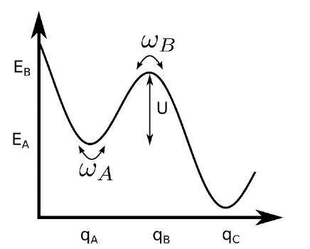
Figure 4: Sketch for the usual reaction rate problem, in terms of a generic reaction coordinate $q$: Two metastable states at $q_{A}$ and $q_{C}$ are connected by a barrier with height $U=E_{B}-E_{A}$ and maximum at $q_{B}$. The curvatures are also shown.

In general the reaction rate can be written as

$$r=k\,e^{-U/k_{\rm B}T}\,,$$ (20)

where the prefactor $k$ depends on the temperature $T$, the friction coefficient or ‘damping’ of the system, and the details of the potential energy function. An accurate estimation of this prefactor has been shown to be a formidable task and many articles have been devoted to this end —deserving an special mention the celebrated one by Kramers Kramers (1940). See also Refs.Pollak and Talkner, 2005; Hänggi et al., 1990; Melnikov, 1991.

As it has been shown in Ref. Alonso et al., 2010 and summarized in the previous sections, the inclusion of excited electronic levels becomes important at certain temperatures for obtaining suitable PESs of molecular systems, different from the gsBO one. The object of this section is to consider the effect of these excited states on the thermal-activation rate calculations.

Let us denote by $r_{\rm eff}$ the activation rate for the effective potential $V_{\rm eff}(q;T)$ in Eq. (II), and by $r_{0}$ the rate for the gsPES, $E_{0}(q)$ (both of them expressed as a function of the reaction coordinate $q$). The main effect of the inclusion of the new terms associated to the excited electronic states is a reduction of the energy barrier from $U_{0}=E_{0}(q_{B})-E_{0}(q_{A})$ to $U_{\rm eff}=V_{\rm eff}(q_{B}^{\rm eff})-V_{\rm eff}(q_{A}^{\rm eff})$. We will have in general $q_{A}^{\rm eff}\simeq q_{A}$ and $V_{\rm eff}(q_{A}^{\rm eff})\simeq E_{0}(q_{A})$, and thus the change in the energy barrier is given by the change at the potential maximum. Regarding the activation rate, in the simplest picture, we find that $r_{\rm eff}\sim e^{-U_{\rm eff}/k_{B}T}$ and $r_{\rm eff}/r_{0}\sim e^{-(U_{\rm eff}-U_{0})/k_{\rm B}T}$. Therefore, if $U_{\rm eff}-U_{0}$ is large enough, the effect of the energy barrier reduction on the activation rate will be important. In addition to this effect, it is also important to realize than the activation rate will also show a deviation from the expected $e^{-U/k_{\rm B}T}$ temperature dependence due to the fact that $U_{\rm eff}$ itself depends on $T$. With this in mind, the importance of the excited electronic states can be studied looking for deviations of $r(T)$ from its expected dependence.

A more detailed analysis must take into account the influence of the prefactor $k$ too. To this end, some approximations need to be done. Let us place our problem in the context of the large-barrier ($U/k_{\rm B}T\gg 1$) and strong-friction limit. In such a situation, we learnt from Kramers that,Kramers (1940)

$$r_{\rm KHD}=\frac{\omega_{A}}{\gamma}\sqrt{\frac{k_{\rm B}T}{2\pi}}\left\{\int_{q_{A}}^{q_{B}}{\rm e}^{U(q)/k_{\rm B}T}dq\right\}^{-1}\,,$$ (21)

where $U(q):=V(q)-V(q_{A})$, being $V(q)$ the appropriate potential. Here, $\omega_{A}$ is associated to the curvature of the potential at point $A$, $\gamma$ is the friction coefficient and KHD stands for Kramers high-damping limit.

This formula can be used directly to calculate the reaction rate by performing the integral numerically, and this is what we will do in this section. However, before doing that, let us introduce two simple approximations that are instructive and give some insights about the general features of the problem. For a large barrier, a narrow region around the maximum gives most of the contribution to the integral. In many cases we can use the so-called parabolic barrier approximationKramers (1940): $U_{\rm near\;B}\simeq U_{B}-\frac{1}{2}\omega_{B}^{2}(q-q_{B})^{2}$. Then

$$r_{\rm KHD}^{\rm pb}\simeq\frac{\omega_{A}\omega_{B}}{2\pi\gamma}e^{-U_{B}/k_{\rm B}T}\,.$$ (22)

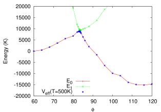
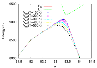
Figure 5: Calculated potential energy profiles for ozone. Top: $E_{0}(\phi)$, $E_{1}(\phi)$ and $V_{\rm eff}(\phi)$ at 500 K. State A lies at $\phi_{A}=60^{o}$ ($E_{0}(\phi_{A})=0$ K) and the barrier is located at approximately $\phi_{B}=83.4^{o}$ ($E_{0}(\phi_{B})=9094$ K). Bottom: Potential profiles close to the barrier. $E_{0}(\phi)$, $E_{1}(\phi)$ and $V_{\rm eff}(\phi)$ for $T=$100, 200, 300, 400 and 500 K.

In this situation, we have

$$\frac{r_{\rm eff}}{r_{0}}\simeq\frac{\omega_{B}^{\rm eff}(T)}{\omega_{B}}e^{-(U_{\rm eff}(T)-U_{0})/k_{\rm B}T}\,.$$ (23)

Now, if $V_{\rm eff}\sim E_{0}$ beyond the barrier and $V_{\rm eff}<E_{0}$ at the barrier, we expect $\omega_{B}^{\rm eff}<\omega_{B}$ (see also the end of Sec. III). Hence, the prefactor effect opposes the exponential one: The rate will typically diminish because of the changes in the prefactor, but it will typically increase due to the changes in the barrier. In any case, given its exponential dependence, the effect of the barrier reduction is expected to be dominant in most cases.

Special care must be taken if the region of the potential close to the barrier (i.e., the one that contributes significantly to the integral in Eq. (21)) cannot be accurately approximated by a parabolic function around its maximum. Another common approximation to compare with is given by a cusp barrier:

$$U_{\rm near\ B}\simeq\begin{cases}U_{B}+m_{1}(q-q_{B})&\quad\mathrm{if}\quad q\leq q_{B}\\ U_{B}-m_{2}(q-q_{B})&\quad\mathrm{if}\quad q>q_{B}\\ \end{cases}$$ (24)

where $m_{1},m_{2}>0$ are the slopes at each side of the barrier. In this case, the activation rate can be written as

$$r_{\rm KHD}^{\rm cb}\simeq\frac{\omega_{A}}{2\pi\gamma}\sqrt{\frac{2\pi}{k_{\rm B}T}}\,\lambda\,e^{-U_{B}/k_{\rm B}T}\,,$$ (25)

where $\lambda:=m_{1}m_{2}/(m_{1}+m_{2})$, and we have

$$\frac{r_{\rm eff}}{r_{0}}\simeq\frac{\lambda^{\rm eff}(T)}{\lambda}e^{-(U_{\rm eff}(T)-U_{0})/k_{\rm B}T}\,.$$ (26)

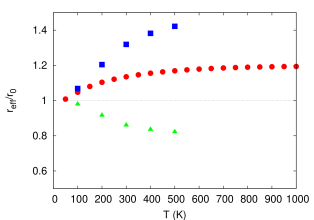
Figure 6: $r_{\rm eff}/r_{0}$ ratio as a function of $T$ (red circles) as computed numerically using Eq. (21). We also show the value of the exponential reduction factor $e^{\delta(T)/k_{\rm B}T}$ (blue squares) and the prefactor change $b(T)$ estimated from Eq. (27) (green triangles).

In conclusion, we can write in both cases

$$\frac{r_{\rm eff}}{r_{0}}\simeq b(T)\ e^{\delta(T)/k_{\rm B}T}\,,$$ (27)

where $\delta(T):=U_{0}-U_{\rm eff}(T)>0$ is the barrier reduction, and $b(T)$ accounts for the changes in the prefactor. For the simplest case where $E_{0}(q)$ and $V_{\rm eff}(q)$ show a maximum at the same coordinate $q_{B}$ (the position of the maximum is not affected by the new terms), it is easy to see that $e^{\delta(T)/k_{\rm B}T}\simeq(1+\ e^{-\Delta/k_{\rm B}T})$ with $\Delta:=E_{1}(q_{B})-E_{0}(q_{B})$, where we have only considered the first excited state $E_{1}$.

As a working case, we will consider now the case of the ring opening reaction of ozone, which has been previously studied in Ref. Alonso et al., 2010. Fig. 5 shows the potential profile for ozone as a function of the opening angle $\phi$ at different temperatures. Since this is enough for our purposes, we consider only the gsBO PES, $E_{0}(\phi)$, and the first excited state one, $E_{1}(\phi)$ —taken from Ref. Alonso et al., 2010, where they where computed using the CASSCF method (complete active-space self-consistent field).Roos (1987) The effective potential $V_{\rm eff}(\phi)$ is constructed with them. As we can clearly see in the bottom graph, the potential profile is modified by the inclusion of the new term corresponding to $E_{1}(\phi)$ only in a narrow region close to the barrier. Also, in this case, the potential barrier is close to 9000 K and thus $U/k_{\rm B}T\gg 1$ for the temperature range of interest, which justifies the basic approximations behind the formulae in this section. However, there exist a clear asymmetry between $E_{0}(\phi)$ and $E_{1}(\phi)$. As a consequence, the barrier location moves with $T$, and the barrier energy reduction $\delta(T)$ does not follow the expected $T$ dependence. In addition, as we can see in Fig. 5, neither the parabolic nor the linear cusp approximations will be suitable to fit the barrier profile close to the maximum. Hence, we have directly used Eq. (21) to numerically compute the $r_{\rm eff}/r_{0}$ ratio of the system. The results are presented in Fig. 6, where we can see that, in spite that the small barrier reduction observed, the activation rate changes up to a 20% upon the inclusion of the excited electronic states. This indicates that the non-adiabatic effects associated with low-lying states should be included in any analysis of this kind if one aims for high accuracy in the predictions. Besides, in the same Fig. 6, we also plot the contributions to the ratio $r_{\rm eff}/r_{0}$ coming from the changes both in the potential barrier heigth and shape. As expected the increase of the rate motivated by the barrier reduction is moderated by the prefactor change. The two effects work against each other, and the exponential dependence on the barrier overcomes the influence of the curvature.

IV Conclusions

In this work, we have shown that the ground-state PES, as defined in the Born–Oppenheimer approximation and typically used for many applications in chemistry, physics and materials science, is not the only electronic state that significantly contributes to the theoretical prediction and calculation of thermodynamic observables at non-zero temperature already for small molecular systems. Although this fact was probably expected by the reader, we provide actual numerical examples of relevant observables being significantly modified by the inclusion of thermally-activated low-lying excited electronic states in real systems at not-too-high temperatures: The average bond length of the Manganase dimer is shown to change in an amount which is accessible to modern experimental techniques, while the reaction rate of the ring opening of ozone is shown to change up to a 20%. Moreover, our compact effective potential, which includes any number of such states and which, despite its simplicity, is able to produce the correct Boltzmann weight for the electronic subsystem —a long sought property in the field of quantum-classical models.

Also, as discussed in section Sec. II, a general result when using our effective potential is that, in any avoided crossing situation, the curvature on the top of the barrier is smaller than the gsPES curvature. As shown in Ref. Bothma et al., 2010, if the curvature is smaller, the tunneling below the energy barrier will occur at lower temperature. Therefore, the inclusion of low-lying electronic states is important if one wants to adequately discriminate possible quantum-like behaviour of the nuclei from simple classical effects due to the direct influence of temperature on the potential —for example in biological systems.Bothma et al. (2010); Iyengar et al. (2008)

Additionally, although the effective potential used in this work has been derived in Ref. Alonso et al., 2010 assuming classical nuclei and equilibrated electrons, it could also be used as an external potential to perform calculations on quantum nuclei. This procedure would allow to study low temperatures, while still including a possible correction due to electronic excitations. Notice, however, that, although the use of the gsPES in the BO approximation as a potential for quantum nuclei can be rigorously justified (see, e.g., Eq. (17) in Ref. Doltsinis and D., 2002), in the case of the effective potential used in this work, its use in this manner is not justified in principle because of its intrinsic non-adiabatic origin.

Finally, it is also reasonable to expect that the use of our temperature dependent effective potential provides new insights that could lead to answer the intriguing question of the thermodynamical stability of some diatomic dications,Corral et al. (2011) an issue we plan to address in the next future.

References

- Born and Oppenheimer (1927) M. Born and J. R. Oppenheimer, “Zur Quantentheorie der Molekeln,” Ann. Phys.-Leipzig, 84, 457 (1927).
- Echenique and Alonso (2007) P. Echenique and J. L. Alonso, “A mathematical and computational review of Hartree–Fock SCF methods in quantum chemistry,” Mol. Phys., 105, 3057 (2007).
- Alonso et al. (2010) J. L. Alonso, A. Castro, P. Echenique, V. Polo, A. Rubio, and D. Zueco, “Ab initio molecular dynamics on the electronic Boltzmann equilibrium distribution,” New J. Phys., 12, 083064 (2010).
- Mazzola et al. (2012) G. Mazzola, A. Zen, and S. Sorella, “Finite temperature electronic simulations beyond the Born-Oppenheimer approximation,” arXiv:1205.4526 (2012).
- Zhu et al. (2005) C. Zhu, A. W. Jasper, and D. G. Truhlar, “Non-Born-Oppenheimer Liouville-von Neumann Dynamics. Evolution of a Subsystem Controlled by Linear and Population-Driven Decay of Mixing with Decoherent and Coherent Switching,” J. Chem. Theory Comput., 1, 527 (2005).
- Truhlar (2007) D. G. Truhlar, “Decoherence in Combined Quantum Mechanical and Classical Mechanical Methods for Dynamics as Illustrated for Non-Born–Oppenheimer Trajectories,” in Quantum Dynamics of Complex Molecular Systems, edited by D. A. Micha and I. Burghardt (Springer, Berlin, 2007) pp. 227–243.
- Schmidt et al. (2008) J. R. Schmidt, P. V. Parandekar, and J. C. Tully, “Mixed quantum-classical equilibrium: Surface hopping,” J. Chem. Phys., 129, 044104 (2008).
- Worth and Ceberbaum (2004) G. A. Worth and L. S. Ceberbaum, Annu. Rev. Phys. Chem., 55, 127 (2004).
- J. Martinez et al. (1996) T. J. Martinez, M. Ben-Nun, and R. D. Levine, J. Phys. Chem., 100, 7884 (1996).
- Nakamura (2002) H. Nakamura, Nonadiabatic Transitions: Concepts, Basic Theories and Applications (World Scientific, 2002).
- Baer (2006) M. Baer, Beyond Born-Oppenheimer: Conical Intersections and Electronic Nonadiabatic Coupling Terms (John Wiley & Sons, 2006).
- Prezhdo (1999) O. Prezhdo, J. Chem. Phys., 111, 8366 (1999).
- Alonso et al. (2011) J. L. Alonso, A. Castro, J. Clemente-Gallardo, J. C. Cuchí, P. Echenique, and F. Falceto, “Statistics and Nosé formalism for Ehrenfest dynamics,” J. Phys. A: Math. Theor., 44, 395004 (2011).
- Alonso et al. (2012) J. L. Alonso, J. Clemente-Gallardo, J. C. Cuchí, P. Echenique, and F. Falceto, “Ehrenfest dynamics is purity non-preserving: a necessary ingredient for decoherence,” arXiv:1205.0885 (2012).
- Bartell (1955) L. S. Bartell, “Effects of Anharmonicity of Vibration on the Diffraction of Electrons by Free Molecules,” J. Chem. Phys., 23, 1219 (1955a).
- Varga et al. (2010) Z. Varga, M. Hargittai, and L. S. Bartell, “On the thermal expansion of molecules,” Struct. Chem., 22, 111 (2010).
- Varga et al. (2011) Z. Varga, M. Hargittai, and L. S. Bartell, “On the thermal expansion of molecules: a sequel,” Struct. Chem., 22, 1065 (2011).
- Bartell (1979) L. S. Bartell, “Bond lengths of vibrationally hot AXn molecules. A simple treatment,” J. Chem. Phys., 70, 4581 (1979).
- Bartell et al. (1979) L. S. Bartell, S. K. Doun, and S. R. Goates, “Inference of vibrational anharmonicity in hot SF{$_6$}: An electron diffraction study,” J. Chem. Phys., 70, 4585 (1979).
- Goates and Bartell (1982) S. R. Goates and L. S. Bartell, “Electron diffraction studies of hot molecules. I. Observed and calculated thermal expansions of SF{$_6$}, CF{$_4$}, and SiF{$_4$},” J. Chem. Phys., 77, 1866 (1982a).
- Goates and Bartell (1982) S. R. Goates and L. S. Bartell, “Electron diffraction studies of hot molecules. II. “Anharmonic shrinkage effects” in SF{$_6$}, CF{$_4$}, and SiF{$_4$},” J. Chem. Phys., 77, 1874 (1982b).
- Bartell et al. (1984) L. S. Bartell, W. Vance, and S. R. Goates, “Electron diffraction studies of hot molecules. III. Stretching and bending anharmonicity in CF{$_3$}Cl,” J. Chem. Phys., 80, 3923 (1984).
- Hänggi et al. (1990) P. Hänggi, P. Talkner, and M. Borkovec, “Reaction-rate theory: fifty years after Kramers,” Rev. Mod. Phys., 62, 251 (1990).
- Fleming et al. (2011) D. G. Fleming, D. J. Arseneau, O. Sukhorukov, J. H. Brewer, S. L. Mielke, D. G. Truhlar, G. C. Schatz, B. C. Garrett, and K. A. Peterson, “Kinetics of the reaction of the heaviest hydrogen atom with h[sub 2], the [sup 4]he mu + h[sub 2] –> [sup 4]he mu h + h reaction: Experiments, accurate quantal calculations, and variational transition state theory, including kinetic isotope effects for a factor of 36.1 in isotopic mass,” J. Chem. Phys., 135, 184310 (2011).
- Bothma et al. (2010) J. P. Bothma, J. B. Gilmore, and R. H. McKenzie, “The role of quantum effects in proton transfer reactions in enzymes: quantum tunneling in a noisy environment?” New J. Phys., 12, 055002 (2010).
- Iyengar et al. (2008) S. S. Iyengar, I. Sumner, and J. Jakowski, “Hydrogen tunneling in an enzyme active site: a quantum wavepacket dynamical perspective,” J. Phys. Chem. B, 112, 7601 (2008).
- Mauri et al. (1993) F. Mauri, R. Car, and E. Tosatti, “Canonical Statistical Averages of Coupled Quantum-Classical Systems,” Europhys. Lett., 24, 431 (1993).
- Kapral and Ciccotti (1999) R. Kapral and G. Ciccotti, “Mixed quantum-classical dynamics,” J. Chem. Phys., 110, 8919 (1999).
- Nielsen et al. (2001) S. Nielsen, R. Kapral, and G. Ciccotti, “Statistical mechanics of quantum-classical systems,” J. Chem. Phys., 115, 5805 (2001).
-
(30)
Let us assume that the
probability distribution function of a hybrid quantum-classical system can
indeed be represented by a “parameterized” density matrix
, where the parameters are the classical variables.
Likewise, any observable can be represented by a parameterized operator
. The average of any observable can be computed as:
Then, the that maximizes the entropy, defined as
subject to the constraints and , is precisely given by Eq. (2.4) in the paper. . - Tzeli et al. (2008) D. Tzeli, U. Miranda, I. G. Kaplan, and A. Mavridis, “First principles study of the electronic structure and bonding of mn[sub 2],” J. Chem. Phys., 129, 154310 (2008).
- Bartell (1955) L. S. Bartell, “Effects of anharmonicity of vibration on the diffraction of electrons by free molecules,” J. Chem. Phys., 23, 1219 (1955b).
- Kuchitsu and Bartell (1962) K. Kuchitsu and L. S. Bartell, “Effect of anharmonic vibrations on the bond lengths of polyatomic molecules. i. model of force field and application to water,” J. of Chem. Phys., 36, 2460 (1962).
- Kuchitsu and Bartell (1961) K. Kuchitsu and L. S. Bartell, “Effects of anharmonicity of molecular vibrations on the diffraction of electrons. ii. interpretation of experimental structural parameters,” J. Chem. Phys., 35, 1945 (1961).
- Toyama et al. (1964) M. Toyama, T. Oka, and Y. Morino, “Effect of vibration and rotation on the internuclear distance,” J. Mol. Spectrosc., 13, 193 (1964), ISSN 0022-2852.
- Herschbach and Laurie (1962) D. R. Herschbach and V. W. Laurie, “Influence of vibrations on molecular structure determinations. i. general formulation of vibration—rotation interactions,” J. Chem. Phys., 37, 1668 (1962).
- Spiridonov et al. (2001) V. Spiridonov, N. Vogt, and J. Vogt, “Determination of molecular structure in terms of potential energy functions from gas-phase electron diffraction supplemented by other experimental and computational data,” Struct. Chem., 12, 349 (2001).
- Butayev et al. (1985) B. S. Butayev, V. P. Spiridonov, A. S. Saakjan, A. Y. Nasarenko, and A. G. Gershikov, “Effects of centrifugal distortion on the distance and amplitude parameters of diatomic molecules,” J. Mol. Struct., 119, 295 (1985).
- Wang and Chen (2004) B. Wang and Z. Chen, “Magnetic coupling interaction under different spin multiplets in neutral manganese dimer: Caspt2 theoretical investigation,” Chem. Phys. Lett., 387, 395 (2004), ISSN 0009-2614.
- Yamamoto et al. (2006) S. Yamamoto, H. Tatewaki, H. Moriyama, and H. Nakano, “A study of the ground state of manganese dimer using quasidegenerate perturbation theory,” J. Chem. Phys., 124, 124302 (2006).
- Arrhenius (1889) S. Arrhenius, Z. Phys. Chem. (Leipzig), 4, 226 (1889).
- Kramers (1940) H. Kramers, Physica (Utrecht), 7, 284 (1940).
- Pollak and Talkner (2005) E. Pollak and P. Talkner, Chaos, 15, 026116 (2005).
- Melnikov (1991) V. I. Melnikov, Phys. Rep., 209, 1 (1991).
- Roos (1987) B. O. Roos, “The complete active space self-consistent field method and its applications in electronic structure calculations,” Adv. Chem. Phys., 69, 399 (1987).
- Doltsinis and D. (2002) N. L. Doltsinis and M. D., J. Theor. Comput. Chem., 1, 319 (2002).
- Corral et al. (2011) I. Corral, A. Palacios, and M. Yanez, “Electronic structure and lifetimes of gax2+ (x = n, o, f) in the gas phase. unraveling stability trends,” Phys. Chem. Chem. Phys., 13, 18365 (2011).