Application of the Gaussian mixture model in pulsar astronomy – pulsar classification and candidates ranking for Fermi 2FGL catalog

Abstract

Machine learning, algorithms to extract empirical knowledge from data, can be used to classify data, which is one of the most common tasks in observational astronomy. In this paper, we focus on Bayesian data classification algorithms using the Gaussian mixture model and show two applications in pulsar astronomy. After reviewing the Gaussian mixture model and the related Expectation-Maximization algorithm, we present a data classification method using the Neyman-Pearson test. To demonstrate the method, we apply the algorithm to two classification problems. Firstly, it is applied to the well known period-period derivative diagram, where we find that the pulsar distribution can be modeled with six Gaussian clusters, with two clusters for millisecond pulsars (recycled pulsars) and the rest for normal pulsars. From this distribution, we derive an empirical definition for millisecond pulsars as $\frac{\dot{P}}{10^{-17}}\leq 3.23\left(\frac{P}{100\,\textrm{ ms}}\right)^{-2.34}$. The two millisecond pulsar clusters may have different evolutionary origins, since the companion stars to these pulsars in the two clusters show different chemical composition. Four clusters are found for normal pulsars. Possible implications for these clusters are also discussed. Our second example is to calculate the likelihood of unidentified Fermi point sources being pulsars and rank them accordingly. In the ranked point source list, the top 5% sources contain 50% known pulsars, the top 50% contain 99% known pulsars, and no known active galaxy (the other major population) appears in the top 6%. Such a ranked list can be used to help the future follow-up observations for finding pulsars in unidentified Fermi point sources.

1 Introduction

A common and important task in observational astronomy is to find or select a certain type of objects from a sample of candidates according to particular physical properties. Examples include selecting active galaxy candidates from a multi-color optical photometry survey, selecting good pulsar candidates from a large number of candidates produced in pulsar searches. Such tasks are time consuming, especially when the number of candidates is large. In this situation, computers can offer significant help when the selection rules can be derived based on prior experiences or physical considerations. However, for some applications, it is hard to determine the a priori criteria and one has to search for the selection criterion using the empirical knowledge embedded in the data themselves. For example, different types of sources usually form clusters in different regions of parameter space. When a large population of candidates is available, the clustering becomes statistically significant, and one can then use this to determine the selection criterion.

In order to build up the empirical selection criterion, we need to find a method to learn the knowledge from the data and apply this to generate the selection rules. Machine learning algorithms are designed to extract empirical knowledge from a sample of data, and improve its performance based on the knowledge it learnt. Machine learning algorithms also contain methods to classify data. There are already many successful applications of machine learning algorithms since the 1960s, some of which were recently used in the pulsar community (e.g. Eatough et al. 2010). We refer to Theodoridis & Koutroumbas (2009) for the details of such algorithms and their applications in broader fields. Clearly, machine learning and related classification algorithms can help to determine the criteria required to select desirable objects from a large sample of candidates in the context of observational astronomy.

This paper demonstrates the application of Gaussian mixture model (GMM) in the context of pulsar astronomy. The GMM, which we use here, is one type of un-supervised learning algorithms based on Bayesian decision theory (Press et al., 2007). It assumes that the data clusters in parameter space follow a superposition of several multivariate Gaussian distributions. The parameters of each cluster are determined from data using the Expectation-Maximization (EM) algorithm. We use two examples to show the application of GMM in pulsar astronomy. Our first example is to classify pulsars in the parameter space of pulsar period ($P$) and period derivative ($\dot{P}$), and the second example is to calculate the likelihood of a gamma-ray point source being a pulsar. Here gamma-ray point source parameters are from the Fermi gamma-ray Space Telescope Large Area Telescope 2-year Point Source Catalog (2FGL catalog, The-Fermi-LAT-Collaboration 2011b).

This article is organized as follows. We introduce the statistical technique, the GMM, in Section 2. We use two problems as examples to show properties and applications of GMM in Section 3. The first application in Section 3.1 is to find an empirical definition for millisecond pulsars (MSPs) from the period-period derivative ($P-\dot{P}$) distribution of known pulsars. The second application in Section 3.2 is to describe the 2FGL catalog point source distribution, to calculate the likelihood of a particular source being a pulsar, and to produce a pulsar candidate list for later confirmation observations. Conclusions and discussions are given in Section 4.

2 Gaussian Mixture Model And Likelihood Ranking

In this section, we introduce the basic concepts of GMM as well as related techniques to classify the data in parameter space.

The GMM is a probabilistic model to describe the distribution of data with clusters in the parameter space, where each cluster is assumed to follow the Gaussian distribution. For a total of $m$ clusters in a $n$-dimensional parameter space, the probability distribution $P({\boldsymbol{{x}}})$ of data ${\boldsymbol{{x}}}$ is given by a weighted summation of all $m$ Gaussian clusters, i.e.

$$P({\boldsymbol{{x}}})=\sum_{k=1}^{m}P_{k}P({\boldsymbol{{x}}}|{\boldsymbol{{\mu}}}_{k},{\boldsymbol{{\Sigma}}}_{k})\,,$$ (1)

where the mixture weight of the $k$-th Gaussian is $P_{k}$ and the distribution of each individual Gaussian cluster is

$$P({\boldsymbol{{x}}}|{\boldsymbol{{\mu}}}_{k},{\boldsymbol{{\Sigma}}}_{k})=\frac{\exp\left[-\frac{1}{2}({\boldsymbol{{x-\mu}}}_{k})\cdot{\boldsymbol{{\Sigma}}}_{k}^{-1}\cdot({\boldsymbol{{x-\mu}}}_{k})\right]}{(2\pi)^{n/2}\sqrt{|{\boldsymbol{{\Sigma}}}_{k}|}}\,.$$ (2)

$|{\boldsymbol{{\Sigma}}}_{k}|$ is the determinant of ${\boldsymbol{{\Sigma}}}_{k}$, the ${\boldsymbol{{\mu}}}_{k}$ and ${\boldsymbol{{\Sigma}}}_{k}$ are the mean vector and co-variance of the $k$-th Gaussian respectively.

The parameters of GMM, i.e. $P_{k}$, ${\boldsymbol{{\mu}}}_{k}$ and ${\boldsymbol{{\Sigma}}}_{k}$, can be determined from the data by an unsupervised machine learning technique, namely the Expectation-Maximization (EM) algorithm (Press et al., 2007), which assumes no prior knowledge about the clustering structures. For $N$ data points ${\boldsymbol{{x_{i}}}}$, where $i=1\ldots N$, the EM algorithm starts from an initial guess and learns GMM parameters from the data. The steps involved are:

• Guess starting values for ${\boldsymbol{{\mu}}}_{k},{\boldsymbol{{\Sigma}}}_{k}$, and $P_{k}$

• Expectation-step (E-step): calculate $P({\boldsymbol{{x}}}|{\boldsymbol{{\mu}}}_{k},{\boldsymbol{{\Sigma}}}_{k})$ and $P({\boldsymbol{{x}}})$ using Equations (1) and (2).

• Maximization-step (M-step): Update model parameters ${\boldsymbol{{\mu}}}_{k},{\boldsymbol{{\Sigma}}}_{k}$ using

  $${\boldsymbol{{\mu_{k,{\rm new}}}}} = \frac{\sum_{i=1}^{N}{\boldsymbol{{x}}}_{i}P_{k}P({\boldsymbol{{x}}}_{i}|{\boldsymbol{{\mu}}}_{k},{\boldsymbol{{\Sigma}}}_{k})/P({\boldsymbol{{x}}}_{i})}{\sum_{i=1}^{N}P_{k}P({\boldsymbol{{x}}}_{i}|{\boldsymbol{{\mu}}}_{k},{\boldsymbol{{\Sigma}}}_{k})/P({\boldsymbol{{x}}}_{i})}\,,$$ (3)

  $${\boldsymbol{{\Sigma_{k,{\rm new}}}}} = \frac{\sum_{i=1}^{N}({\boldsymbol{{x}}}_{i}-{\boldsymbol{{\mu}}}_{k})\otimes({\boldsymbol{{x}}}_{i}-{\boldsymbol{{\mu}}}_{k})P_{k}P({\boldsymbol{{x}}}_{i}|{\boldsymbol{{\mu}}}_{k},{\boldsymbol{{\Sigma}}}_{k})/P({\boldsymbol{{x}}}_{i})}{\sum_{i=1}^{N}P_{k}P({\boldsymbol{{x}}}_{i}|{\boldsymbol{{\mu}}}_{k},{\boldsymbol{{\Sigma}}}_{k})/P({\boldsymbol{{x}}}_{i})}\,,$$ (4)

  $$P_{k,{\rm new}} = \frac{1}{N}\sum_{i=1}^{N}P_{k}P({\boldsymbol{{x}}}_{i}|{\boldsymbol{{\mu}}}_{k},{\boldsymbol{{\Sigma}}}_{k})/P({\boldsymbol{{x}}}_{i})\,,$$ (5)

  where $i$ is the index for data points. $\otimes$ is the symbol for ‘outer product’, i.e. for any vectors ${\boldsymbol{{x}}}$ and ${\boldsymbol{{y}}}$, ${\boldsymbol{{x}}}\otimes{\boldsymbol{{y}}}$ is the matrix, of which the $\nu$-th row $\mu$-th column element is the product of the $\nu$-th element of ${\boldsymbol{{x}}}$ and the $\mu$-th element of ${\boldsymbol{{y}}}$.

• Repeat the EM steps, until the total likelihood $\Lambda$ converges, where

  $$\Lambda=\prod_{i=1}^{N}P({\boldsymbol{{x}}}_{i})\,.$$ (6)

It can be shown that the above iteration of the EM algorithm increases the total likelihood $\Lambda$, and the iterations always converge .

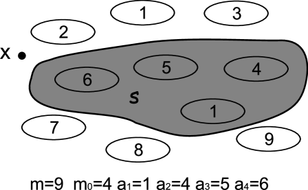
Figure 1: An illustration of the definition of the GMM and data clustering. The ${\boldsymbol{{x}}}$ indicates a data point. The index for each Gaussian is labeled. Here the total number of Gaussian clusters is $m=9$, where four of them belong to the subset $\cal S$ ($m_{0}=4$), as indicated by the shaded area, thus ${\boldsymbol{{x}}}\notin{\cal S}$

With the GMM and its parameters, one can infer the association of any data point ${\boldsymbol{{x}}}$ with these clusters. One can also ask if ${\boldsymbol{{x}}}$ belongs to a certain subset $\cal S$, which contains $m_{0}$ Gaussian clusters out of a total of $m$ Gaussian clusters. An illustration of the definitions is presented in Figure 1, where the indexes of Gaussian clusters in $\cal S$ are $a_{\rm k}$, and $k=1\dots m_{0}$. The question of association can be answered via the standard likelihood ratio test. The Neyman-Pearson lemma (Kassam, 1988) claims that the most powerful test for the binary hypotheses:

$$\left\{\begin{array}[]{c}\textrm{$H_{1}$: ${\boldsymbol{{x}}}$ belongs to subset $\cal S$\,;}\\ \textrm{$H_{0}$: ${\boldsymbol{{x}}}$ belongs to other clusters \,,}\end{array}\right.$$ (7)

is to compare the logarithmic likelihood ratio $\log R_{\cal S}$ against a statistical decision threshold $\eta$, i.e. choose $H_{0}$, if $\log R_{\cal S}\geq\eta$, otherwise choose $H_{1}$. According to the GMM, the logarithmic likelihood ratio $R_{\cal S}$ is

$$\log R_{\cal S}=\log\left(\frac{\sum_{k\in{\cal S}}P_{k}P({\boldsymbol{{x}}}|{\boldsymbol{{\mu}}}_{k},{\boldsymbol{{\Sigma}}}_{k})}{\sum_{k\notin{\cal S}}P_{k^{\prime}}P({\boldsymbol{{x}}}|{\boldsymbol{{\mu}}}_{k^{\prime}},{\boldsymbol{{\Sigma}}}_{k^{\prime}})}\frac{\sum_{k^{\prime}\notin{\cal S}}P_{k^{\prime}}}{\sum_{k\in{\cal S}}P_{k}}\right)\,,$$ (8)

where summation $\sum_{k\in{\cal S}}$ sums over the index $k$ for those clusters in the subset $\cal S$ and $\sum_{k\notin{\cal S}}$ sums over the complementary set of $\cal S$, i.e. those clusters not in the subset $\cal S$.

The number of Gaussian clusters $m$, as an input parameter, can be determined using statistical methods. In practice, one usually starts from $m=1$, and then increases $m$. As $m$ is increased, one can describe the data better. To avoid over-fitting, it is necessary to check the modelling using the multi-dimensional Kolmogorov-Smirnov test (K-S test). Similar to a 1-D K-S test, the multi-dimensional K-S test is used to test whether two data set differ significantly from each other or whether a data set differs from a known distribution. The statistic ($\cal D$) for K-S test is the maximal difference between the cumulative distribution of two data sets or between the data and the model. However, the cumulative distribution of multi-dimensional data is not well defined, thus it was proposed to compute such ‘cumulative distribution’ for any possible order and then calculate the $\cal D$. For example, in order to determine the maximal difference $\cal D$ between data and data or between data and distribution, it is necessary to check the cumulative probability for all of the four cases $(x<x_{i},y<y_{i}),(x<x_{i},y>y_{i}),(x>x_{i},y<y_{i})$, and $(x>x_{i},y>y_{i})$ for any data point $(x_{i},y_{i})$ belonging to the two dimensional data set ${\boldsymbol{{x}}}=(x_{i},y_{i}),i\in[1,N]$. For a multi-dimensional K-S test, the statistical threshold and p-values are usually calculated numerically via Monte-Carlo simulation, which generates the mock data sets and calculates the null-hypothesis distribution of $\cal D$ accordingly. We refer readers to Peacock (1983) and Fasano & Franceschini (1987) for more details of such tests.

In summary, the technique of using the GMM to describe a data distribution and to determine the data association is given in the following recipe:

1. Determine the parameter space and form the data vector ${\boldsymbol{{x}}}$ for the data set.

2. Guess the number of clusters $m$ and their initial parameters, i.e. ${\boldsymbol{{\mu}}}_{k}$ and ${\boldsymbol{{\sigma}}}_{k}$, where $k=1\dots m$.

3. Use the EM algorithm to find the true model parameters.

4. Check if GMM describes the data distribution well enough using the multi-dimensional Kolmogorov-Smirnov test. Increase the number of Gaussian clusters, if the test fails.

5. Once the model parameters are found, use Equation (8) to determine the data association.

We present two examples in next section to show its applications.

3 Application

3.1 Application to pulsar classification

As the first example, we apply GMM to the well-known pulsar $P-\dot{P}$ diagram to find a quantitative description for the pulsar distribution. We also seek the ‘empirical MSP definition’ here, especially because a precise definition for MSPs using their periods and period derivatives is not available yet.

The standard picture for pulsar evolution contains several major stages, i) the birth of pulsar in a supernova explosion, ii) the spin-down of pulsar due to radiation energy loss, iii) the pulsar death due to the decrease in radiation power, and possibly for some binary system, iv) the pulsar recycling by accretion induced spin-up. After birth in the supernova, the young pulsars usually have short periods and large period derivatives. They occupy the upper left part of the $P-\dot{P}$ diagram, and are frequently associated with supernova remnants. As the pulsars age, they slow down, while, for those pulsars with breaking index $n=2-\ddot{P}P/\dot{P}^{2}>2$, their $\dot{P}$ also decreases. The pulsars then enter the main population in the centre of the diagram, referred to as the normal pulsars. Eventually such spin-down causes the death of pulsars, i.e.  the radiation of pulsar ceases or becomes too weak to detect. Pulsars may also get recycled via the accretion process (Bhattacharya & van den Heuvel, 1991). The millisecond pulsars (MSPs), which occupy the lower left corner of the $P-\dot{P}$ diagram, are commonly believed to form due to such a spin-up of a normal pulsar via accretion materials from a companion stars. A continuum of pulsars from the MSP population to the normal pulsar population is already observed, where the intermediate population are referred to as mildly recycled pulsars. There are also pulsars occupying the upper right part of the $P-\dot{P}$ diagram. The origin and evolution of these high magnetic field pulsars is still unclear.

We use pulsar $P$ and $\dot{P}$ values from the ATNF pulsar catalogue (Manchester et al., 2005). The distribution of pulsars is plotted in Figure 2. The distribution of the whole pulsar population does not follow a Gaussian distribution, but we can approximate the overall distribution with multiple Gaussian clusters, i.e. the GMM is still valid for the modelling purposes. We apply the GMM in the $P-\dot{P}$ diagram, so our parameter vector ${\boldsymbol{{x}}}$ is

$${\boldsymbol{{x}}}=\log\left(\begin{array}[]{c}P\\ \dot{P}\end{array}\right)\,.$$ (9)

We directly apply the GMM to the data set. The EM algorithm for GMM is stable so the EM algorithm converges for most initial values, although the EM algorithm does not guarantee that it converges to the best global maximum of the total likelihood $\Lambda$. In order to attain the global maximum, initial GMM parameters are generated randomly from a uniform distribution covering the whole $P-\dot{P}$ diagram (in particular,we choose the range of $P$ from $10^{-4}$ to 20 s, and the range of $\dot{P}$ from $10^{-22}$ to $10^{-10}$). We then use these initial parameters in the EM algorithm. We repeat this process $10^{4}$ times to determine the best global model parameters giving the largest likelihood value. In this case, the probability to converge to the best model is more than 30% for all guesses. The GMM is tested using the multi-dimensional Kolmogorov-Smirnov test (Peacock, 1983; Fasano & Franceschini, 1987), for which the $p$-value is chosen to be 95%. To pass such test, we need six different Gaussian components in the GMM.

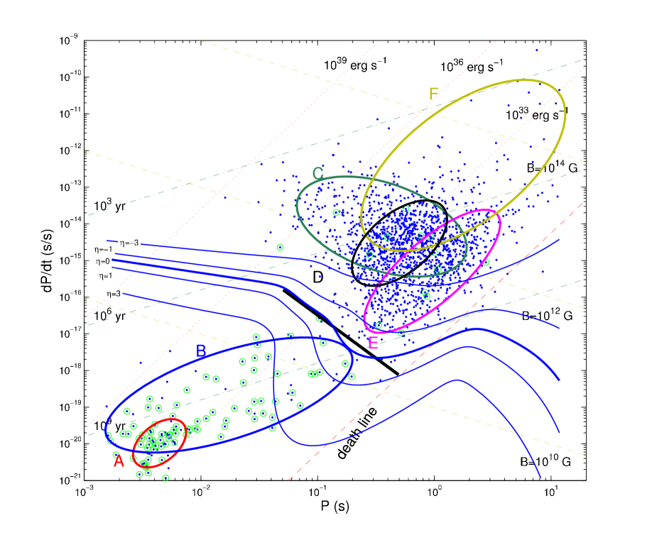
Figure 2: The pulsar $P$-$\dot{P}$ diagram. Elliptic curves are $2-\sigma$ contours for the six Gaussian clusters found by GMM. Dots are all detected pulsars from the ATNF catalogue, and those with circles are binaries. Blue curves with numerical labels on the left ends are contours for equal logarithmic likelihood $\log(R_{\cal S})$. The definition of MSP according to our model is $\log R_{\cal S}\leq 0$, which is plotted with thick blue line. The linear approximation of $\log R_{\cal S}=0$ with $50\,\textrm{ms}\leq P\leq 0.5\,\textrm{s}$ (i.e. Equation (10)) is plotted using a thick black straight line. Lines with equal magnetic field strength, spin-down power, characteristic age as well as the death line are also plotted. Data are from the ATNF pulsar catalogue (Manchester et al. 2005, http://www.atnf.csiro.au/research/pulsar/psrcat/).

Table 1: Numerical values of the GMM parameters for the pulsar distribution in the $P-\dot{P}$ space. The definitions are in Equations (1) and (2). The mixture weights, $P_{A}\dots P_{F}$, as probabilities, are dimensionless. The central vectors of clusters, ${\boldsymbol{{\mu}}}_{A}\dots\boldsymbol{{\mu}}_{F}$, have the same units with respect to ${\boldsymbol{{x}}}$, i.e. $(\log($s$)$, $\log($s/s$))$. The covariance matrices ${\boldsymbol{{\Sigma}}}_{A}\dots\boldsymbol{{\Sigma}}_{F}$ are in the linear space of ${\boldsymbol{{x}}}\bigotimes{\boldsymbol{{x}}}$, so their units are $\left(\begin{array}[]{c c}\log(\textrm{s})^{2}&\log(\textrm{s})\log(\textrm{s/s})\\ \log(\textrm{s})\log(\textrm{s/s})&\log(\textrm{s/s})^{2}\end{array}\right).$

Name	Value
$P_{A}$	0.0326
$P_{B}$	0.0403
$P_{C}$	0.2474
$P_{D}$	0.3170
$P_{E}$	0.3337
$P_{F}$	0.0290
${\boldsymbol{{\mu}}}_{A}$	$\left(\begin{array}[]{l l}$-$2.3541&$-$19.9847\end{array}\right)$
${\boldsymbol{{\mu}}}_{B}$	$\left(\begin{array}[]{l l}$-$1.7597&$-$18.6687\end{array}\right)$
${\boldsymbol{{\mu}}}_{C}$	$\left(\begin{array}[]{l l}$-$0.4502&$-$14.0749\end{array}\right)$
${\boldsymbol{{\mu}}}_{D}$	$\left(\begin{array}[]{l l}$-$0.2983&$-$14.5266\end{array}\right)$
${\boldsymbol{{\mu}}}_{E}$	$\left(\begin{array}[]{l l}$-$0.0179&$-$15.2945\end{array}\right)$
${\boldsymbol{{\mu}}}_{F}$	$\left(\begin{array}[]{l l}0.2477&$-$12.4064\end{array}\right)$
${\boldsymbol{{\Sigma}}}_{A}$	$\left(\begin{array}[]{l l}0.0172&0.0229\\ 0.0229&0.1451\end{array}\right)$
${\boldsymbol{{\Sigma}}}_{B}$	$\left(\begin{array}[]{l l}0.3732&0.3388\\ 0.3388&0.8204\end{array}\right)$
${\boldsymbol{{\Sigma}}}_{C}$	$\left(\begin{array}[]{l l}0.1764&$-$0.1382\\ $-$0.1382&0.6213\end{array}\right)$
${\boldsymbol{{\Sigma}}}_{D}$	$\left(\begin{array}[]{l l}0.0552&0.0886\\ 0.0886&0.4530\end{array}\right)$
${\boldsymbol{{\Sigma}}}_{E}$	$\left(\begin{array}[]{l l}0.1131&0.2524\\ 0.2524&0.9418\end{array}\right)$
${\boldsymbol{{\Sigma}}}_{F}$	$\left(\begin{array}[]{l l}0.2547&0.4106\\ 0.4106&1.8187\end{array}\right)$

We check the ‘robustness’ of GMM parameters using an algorithm similar to the bootstrap method. The original $P-\dot{P}$ data are re-sampled with replacements to form $10^{2}$ simulated data sets, i.e.  any data point has the same probability of being sampled at any time. The EM algorithm is then applied to these newly simulated data sets and check the stability of GMM parameters as a function of the total number of data points in each simulated data set. We find that there is no significant change in the structure of the Gaussian clusters, if we randomly remove less than 3% of the data. We also have checked the GMM parameter stability with respect to the Shklovskii effect (Shklovskii, 1970), an effect that increases the observed period derivative of the pulsar due to its transverse velocity. The differences between GMM parameters for pulsar distributions with and without correcting the Shklovskii effect are less than 1% (the corrected $\dot{P}$ values are also from the ATNF catalogue). Since the Shklovskii correction is not substantial for the GMM, we ignore it in the rest of the discussions. One needs to re-do the above analysis to further check the stability and robustness of the model parameters, when more pulsar data becomes available.

As plotted in Figure 2, in order to describe the pulsar distribution in the $P-\dot{P}$ diagram, six Gaussian clusters are required, the parameters of which are listed in Table 1. It is clear that two Gaussian clusters (components ‘A’ and ‘B’) are required for describing the MSP distribution and four clusters (components ‘C’, ‘D’,‘E’, and ‘F’) are required for normal pulsars. We calculate the likelihood ratio according to Equation (8), where the set $\cal S$ contains the two MSP clusters. We plot the equal likelihood ratio contours corresponding to $R_{\cal S}=\eta$ in Figure 2. Any of these curves divides the $P-\dot{P}$ diagram into two regions, one for MSPs and the other for normal pulsars. We can now empirically define MSPs as pulsars satisfying $R_{\cal S}\geq 0$. We can derive a linear approximation in $\log P$ to $R_{\cal S}=0$. In order to avoid having regions, where only very few pulsars are present, the linear approximation can be confined to the interesting range of $P$, i.e. the linear approximation is calculated for $P$ from $50$ ms to $0.5$ s as

$$\frac{\dot{P}}{10^{-17}}\leq 3.23\left(\frac{P}{100\,\textrm{ ms}}\right)^{-2.34}\,.$$ (10)

This can be seen as an empirical ‘definition’ for MSPs.

Individual Gaussian clusters may be artifacts, due to an intrinsic pulsar distribution that is non-Gaussian. In this case, multiple components are required to describe the distribution. Such non-Gaussian distribution may come from selection effects in pulsar searching or pulsar evolutionary mechanisms. However, we would like to mention a few interesting features here, which may agree with other evidence.

There are two possible MSP clusters. As shown in Figure 2, the principal axes with maximal eigenvalue for component ‘A’ is parallel to constant energy losing rate lines (defined by $\dot{E}=4\pi^{2}I\dot{P}P^{-3}=3.9\times 10^{46}\left({P}/{\textrm{ s}}\right)^{-3}{\dot{P}}$ erg) , while the principal axes with maximal eigenvalue of component ‘B’ is parallel to the equal characteristic age lines (defined by $\tau_{\rm c}=0.5\,P\dot{P}^{-1}$). Such different directions of eigenvectors may indicate that the MSPs have two different origins or evolutionary tracks, which is supported by the fact that that nearly all component-‘A’ pulsars are He-white dwarf binaries, while the major population in component ‘B’ are CO-white dwarf binaries (Tauris, 2011).

Component ‘B’ contains mildly recycled pulsars, which have larger period and higher magnetic field than other MSPs. According to the GMM, there is no statistical evidence for a separate cluster of mildly recycled pulsars in the $P-\dot{P}$ diagram. This may indicate a ‘smooth spectrum’ for the amount of accreted mass for fully recycled and mildly recycled MSPs, otherwise we would expect a more complex structure in component ‘B’.

There are possibly four normal pulsar clusters. One each for high magnetic field pulsars (component ‘F’), old pulsars close to the death line (component ‘E’), young pulsars (component ‘C’), and middle age pulsars (component ‘D’). Principal axes directions of these ellipses for middle age pulsars, old pulsars, and high magnetic field pulsar are nearly parallel (within $\sim 3^{\circ}$). Such agreement indicates certain common mechanisms among these pulsars, because the probability of three random Gaussian clusters having parallel principal axes within $3^{\circ}$ is by chance small as $(3/90)^{2}\simeq 10^{-3}$.

The young pulsar ellipse ‘C’ is clockwise rotated by $\sim 15^{\circ}$ with respect to the average principal axis directions of ellipses ‘D’, ‘E’, and ‘F’ . Such a rotation may come from the selection effect that it is easier to find bright pulsars. Bearing this selection effect in mind, this rotation may indicate that the old pulsars and the young pulsars have different radiation or evolution mechanisms, which is supported by both the timing and polarization properties. Timing results (Espinoza et al., 2011) show that pulsars with glitch behavior correlates with clusters ‘C’, while the polarization measurements (Weltevrede & Johnston, 2008) indicate that the polarization behaviors for high and low $\dot{E}$ pulsar are different.

We also notice that the ellipse for high magnetic field pulsars is quite extended instead of being localized to only high magnetic field pulsars. It covers regions of both young pulsars and middle age pulsars. This indicates potential links between the high magnetic field population and normal pulsars, for which, some observational evidence already suggests that high magnetic field pulsars may evolve from young pulsars (Lyne, 2004; Lin & Zhang, 2004; Espinoza et al., 2011).

3.2 Application to classification of Fermi point sources

We now apply the GMM to the 2FGL catalog to demonstrate the use of GMM to rank candidates according to likelihood. As already pointed out by Abdo et al. (2010) and The-Fermi-LAT-Collaboration (2011a), one can use the variability and the spectrum information to classify Fermi point sources. In the 2FGL catalog, the Variability_Index ($V\!I$) and Signif_Curve (significance of the fit improvement using a curved spectrum, $Sc$) are used to describe the variability and spectral shape. Figures 3 show that Fermi point sources form two distinctive classes, the pulsars and the active galaxies (AGs), where pulsars usually have smaller $V\!I$ but larger $Sc$ compared to AGs.

Although it is straightforward in classifying, one still needs to be careful using parameters $V\!I$ and $Sc$, since both $V\!I$ and $Sc$ correlate with the Test Statistics (see Abdo et al. 2010 for the definition). Such correlation smears clustering structures at low detection significance. One way to deal with this situation is by re-defining $V\!I$ and $Sc$ to reduce the correlation (The-Fermi-LAT-Collaboration, 2011a). Here, we take an alternative approach, in which the gamma-ray flux is included as an additional parameter to directly correct the correlation. In other words, instead of using only $V\!I$ and $Sc$, we use three variables, $V\!I$, $Sc$, and integral gamma-ray flux from 1 to 100 GeV, ‘Flux1000’ ($F_{1000}$) to classify data. Figures 3 show that pulsars and AGs have different dependence in gamma-ray flux, which helps us in data classification.

We now turn to details of our setup for the GMM. The parameter space we used in the GMM algorithm is spanned by $Sc$, base-10 logarithms of $V\!I$ and $F_{1000}$, i.e. the components of data vector ${\boldsymbol{{x}}}$ are:

$${\boldsymbol{{x}}}=\left(\begin{array}[]{c}\log F_{1000}\\ \log V\!I\\ Sc\end{array}\right)\,.$$ (11)

The distribution of ${\boldsymbol{{x}}}$ for the all 2FGL catalog sources is plotted in Figure 3. The GMM is then applied to the whole population to determine the model parameters. To test the robustness of the algorithm and to check if the result is sensitive to initial values, we run the EM algorithm with randomly generated initial values as in the previous example. We get three Gaussian clusters, where one of the Gaussian clusters overlaps with the AGs, one overlaps with pulsars, and one is for sources with low fluxes. The GMM parameters turn out to be insensitive to initial values. We note that extra Gaussian components are needed to model the details of the low flux branch to pass the multidimensional Kolmogorov-Smirnov test. Such a requirement is simply due to the fact that $Sc\geq 0$, where such a boundary needs more Gaussian components to approximate the distribution. We have also checked that including these extra components will not significantly alter our results of source classification, thus for simplicity we prefer to use only three Gaussian clusters here. The projected 3-$\sigma$ contours of clusters are shown in Figure 3. The GMM parameters, i.e. ${\boldsymbol{{\mu}}}$ and ${\boldsymbol{{\Sigma}}}$, are given in Table 2.

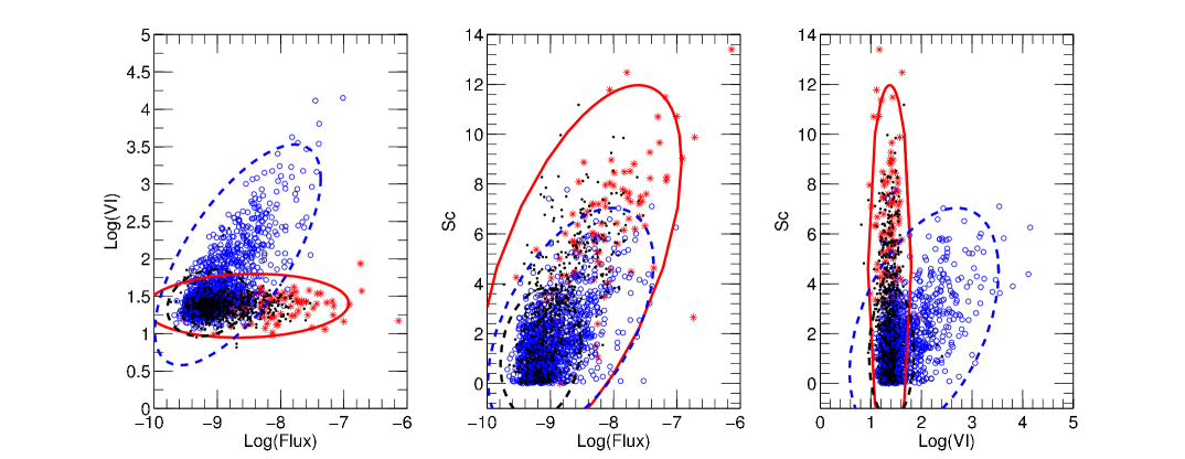
Figure 3: The projected Gaussian clusters and source distribution. Blue ‘$\circ$’ symbols are AGs, red ‘$*$’ symbols are pulsars, un-associated sources are plotted with black solid dots. The units we use for each axis is identical to that in the 2FGL catalog, where the $F_{1000}$ takes the unit of $\rm cm^{-2}\,s^{-1}$. The significance of curved spectrum and variability index are dimensionless according to the 2FGL catalog. There is a 3-D movie of this figure available at http://www.mpifr-bonn.mpg.de/staff/kjlee/gmm.html.

Table 2: GMM parameters for point source distribution in the 2FGL catalog. Similar to Table 1, the $P_{1}\dots P_{3}$ are dimensionless. The vectors ${\boldsymbol{{\mu}}}_{1}\dots\boldsymbol{{\mu}}_{3}$ have the same units with respected to ${\boldsymbol{{x}}}$, i.e. $\left(\log(\textrm{cm}^{-2}\textrm{s}^{-1}),\textrm{dimensionless},\textrm{dimensionless}\right)$. The matrices ${\boldsymbol{{\Sigma}}}_{1}\dots\boldsymbol{{\Sigma}}_{3}$ take units of $\left(\begin{array}[]{c c c}\log(\textrm{cm}^{-2}\textrm{s}^{-1})^{2}&\log(\textrm{cm}^{-2}\textrm{s}^{-1})&\log(\textrm{cm}^{-2}\textrm{s}^{-1})\\ \log(\textrm{cm}^{-2}\textrm{s}^{-1})&\textrm{dimensionless}&\textrm{dimensionless}\\ \log(\textrm{cm}^{-2}\textrm{s}^{-1})&\textrm{dimensionless}&\textrm{dimensionless}\end{array}\right)$

Name	Value
$P_{1}$	0.2856
$P_{2}$	0.2290
$P_{3}$	0.4855
${\boldsymbol{{\mu}}}_{1}$	$\left(\begin{array}[]{l l l}$-$8.5330&1.3732&4.6445\end{array}\right)$
${\boldsymbol{{\mu}}}_{2}$	$\left(\begin{array}[]{l l l}$-$8.6773&2.0533&2.4719\end{array}\right)$
${\boldsymbol{{\mu}}}_{3}$	$\left(\begin{array}[]{l l l}$-$9.1534&1.4110&1.2071\end{array}\right)$
${\boldsymbol{{\Sigma}}}_{1}$	$\left(\begin{array}[]{l l l}2.8686\textrm{e}$-$01&5.9415\textrm{e}$-$03&7.5103\textrm{e}$-$01\\ 5.9415\textrm{e}$-$03&2.0322\textrm{e}$-$02&1.9244\textrm{e}$-$03\\ 7.5103\textrm{e}$-$01&1.9244\textrm{e}$-$03&5.9513\textrm{e}$+$00\\ \end{array}\right)$
${\boldsymbol{{\Sigma}}}_{2}$	$\left(\begin{array}[]{l l l}1.9069\textrm{e}$-$01&1.4785\textrm{e}$-$01&3.3875\textrm{e}$-$01\\ 1.4785\textrm{e}$-$01&2.4183\textrm{e}$-$01&3.2970\textrm{e}$-$01\\ 3.3875\textrm{e}$-$01&3.2970\textrm{e}$-$01&2.3165\textrm{e}$+$00\\ \end{array}\right)$
${\boldsymbol{{\Sigma}}}_{3}$	$\left(\begin{array}[]{l l l}4.5017\textrm{e}$-$02&5.9696\textrm{e}$-$03&2.9135\textrm{e}$-$02\\ 5.9696\textrm{e}$-$03&2.2089\textrm{e}$-$02&3.3940\textrm{e}$-$03\\ 2.9135\textrm{e}$-$02&3.3940\textrm{e}$-$03&7.7004\textrm{e}$-$01\\ \end{array}\right)$

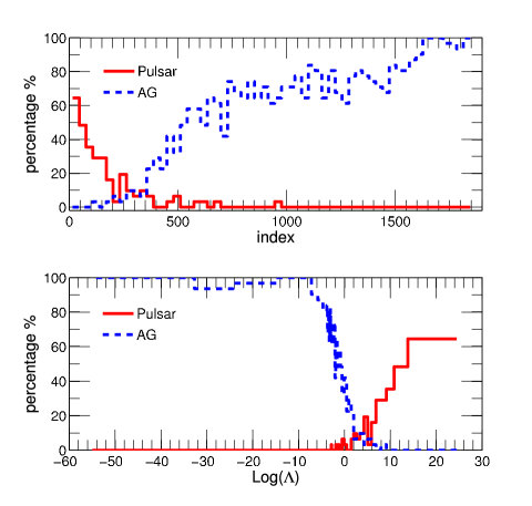
Figure 4: Upper panel: The proportion of pulsars and AGs as functions of ranking index. We bin all the 2FGL catalog sources into 60 bins according to the ranking index. The X-axis is the average index value, and the Y-axis is the proportion of pulsars/AGs in the bin. The solid line is for pulsars, while the dashed line is for AGs. One can see that our algorithm statistically ranks pulsars higher than AGs. Lower panel: The proportion of pulsars and AGs as functions of logarithms of pulsar likelihood. The X-axis is the average logarithm of pulsar likelihood, and the Y-axis is the proportion of pulsars/AGs in each bin. Due to our definition for the likelihood, the proportion of pulsars and AGs equals to each other are at $\log R_{\cal S}=0$, as expected.

Our pulsar likelihood is calculated using Equation (8) with ${\boldsymbol{{\mu}}}_{k}$ and ${\boldsymbol{{\Sigma}}}_{k}$ from Table 2. We identify the pulsar subset $\cal S$ as the pulsar cluster, the complementary set are the AG and low flux cluster. The reason we exclude the low flux cluster from subset $\cal S$ is to suppress candidates with low detection significances.

We sort the 2FGL catalog point sources according to the pulsar likelihood. The whole sorted source list can be found in the online supplement materials of this paper. The first 5 and the last 5 sources are given as examples in Table 3.

In order to verify the validity of our ranking technique, we checked the ranking index of known pulsars and other known sources in our list. To identify pulsars, we used the ‘Public List of LAT-Detected Gamma-Ray Pulsars’, which lists the pulsars that have been detected as pulsed gamma-ray sources with the Fermi LAT up to now. For AGs, the association information is from the 2FGL catalog, i.e. the ‘CLASS1’ entry. Such a comparison is legitimate, since we do not use any information about known pulsar and AG population in the process of finding the model parameters. The comparisons between the ranking results and known population are shown in Figure 4. We can see that the ranking technique separates the pulsar population and AG population. The proportion of pulsars decreases and the proportion of the AGs increases with the ranking index respectively. The top 5% sources contain 50% known pulsars, the top 50% contain 99% known pulsars, and no known active galaxy appears in the top 6%. As predictions, we list the potential pulsar candidates in Table 4, which according to our likelihood are highly pulsar-like objects with no associated sources in the 2FGL catalog. We hope future pulsar searching will benefit from this information.

Table 3: A sample of the source list sorted according to our likelihood. In this list, 2FGL name and corresponding 1FGL name of the sources are given. The source associations are from the 2FGL, and $\log(R_{\cal S})$ is our logarithmic likelihood.

Index	2FGL name	1FGL name	RA (J2000)	DEC (J2000)	Association	$\log R_{\cal S}$
1	2FGL J0633.9$+$1746	1FGL J0633.9$+$1746	06:33:55	$+$17:46:26	PSR J0633$+$1746	$55.8$
2	2FGL J0835.3$-$4510	1FGL J0835.3$-$4510	08:35:21	$-$45:10:45	PSR J0835$-$4510	$52.6$
3	2FGL J1801.3$-$2326e		18:01:22	$-$23:26:24	SNR G006.4$-$00.1	$38.2$
4	2FGL J1836.2$+$5926		18:36:16	$+$59:26:01	LAT PSR J1836$+$5925	$33.0$
5	2FGL J0007.0$+$7303	1FGL J0007.0$+$7303	00:07:06	$+$73:03:16	LAT PSR J0007$+$7303	$30.0$
…	…	…	…	…	…	…
1869	2FGL J0238.7$+$1637	1FGL J0238.6$+$1637	02:38:42	$+$16:37:26	AO 0235$+$164	$-112$
1870	2FGL J1229.1$+$0202	1FGL J1229.1$+$0203	12:29:06	$+$02:02:30	3C 273	$-119$
1871	2FGL J1512.8$-$0906	1FGL J1512.8$-$0906	15:12:50	$-$09:06:12	PKS 1510$-$089	$-139$
1872	2FGL J1224.9$+$2122	1FGL J1224.7$+$2121	12:24:54	$+$21:22:48	4C $+$21.35	$-176$
1873	2FGL J2253.9$+$1609	1FGL J2253.9$+$1608	22:53:59	$+$16:09:09	3C 454.3	$-181$

Table 4: A sample of pulsar candidates sorted according to the pulsar likelihood. The 2FGL name with ${\dagger}$ indicate that there is a known pulsar within the error ellipses of the pointing according to the ATNF pulsar catalogue. The SemiMajor and SemiMinor axes are the source positions at 68% confidence in units of degrees. The column ‘Class’ denotes the possible association of the source, where ‘SNR’ denotes supernova remnant, ‘GLC’ denotes globular cluster, and ‘SPP’ denotes special cases which may associated with SNR or pulsar wind nebula (The-Fermi-LAT-Collaboration, 2011b).

Index	2FGL name	1FGL name	RA	DEC	SemiMajor	SemiMinor	$\log R_{\cal S}$	Class
			J2000	J2000	$10^{-2}\,$deg	$10^{-2}\,$deg
1	2FGL J1801.3$-$2326e		18:01:22	$-$23:26:24	—	—	38.2	SNR
2	2FGL J1745.6$-$2858		17:45:42	$-$28:58:42	1.0	1.0	29.0	SPP
3	2FGL J1855.9$+$0121e		18:55:58	$+$01:21:18	—	—	27.5	SNR
4	2FGL J0617.2$+$2234e	1FGL J0617.2$+$2233	06:17:14	$+$22:34:47	—	—	27.1	SNR
5	2FGL J1906.5$+$0720	1FGL J1906.6$+$0716c	19:06:35	$+$07:20:33	3.5	2.9	18.2
6	2FGL J1923.2$+$1408e		19:23:16	$+$14:08:42	—	—	18.0	SNR
7	2FGL J1045.0$-$5941	1FGL J1045.2$-$5942	10:45:00	$-$59:41:31	1.5	1.4	17.7
8	2FGL J1704.9$-$4618		17:04:59	$-$46:18:14	15.9	11.1	16.6
9	2FGL J0848.7$-$4324		08:48:45	$-$43:24:24	9.4	6.9	16.5
10	2FGL J1738.9$-$2908		17:38:57	$-$29:08:24	15.1	6.6	15.7	SPP
11	2FGL J1819.3$-$1523	1FGL J1819.4$-$1518c	18:19:21	$-$15:23:29	7.4	5.5	15.5
12	2FGL J1747.3$-$2825c		17:47:24	$-$28:25:52	3.6	3.2	15.4
13	2FGL J1805.6$-$2136e		18:05:38	$-$21:36:42	—	—	15.4	SNR
14	†2FGL J1748.0$-$2447	1FGL J1747.9$-$2448	17:48:00	$-$24:47:04	2.3	2.2	14.8	GLC
15	2FGL J2018.0$+$3626		20:18:03	$+$36:26:54	3.7	3.1	14.3
16	2FGL J1839.0$-$0539		18:39:04	$-$05:39:21	1.7	1.6	14.2
17	2FGL J1901.1$+$0427		19:01:11	$+$04:27:27	7.1	5.7	14.1
18	2FGL J1748.6$-$2913	1FGL J1748.3$-$2916c	17:48:39	$-$29:13:52	4.1	3.5	13.8
19	2FGL J1932.1$+$1913	1FGL J1932.1$+$1914c	19:32:10	$+$19:13:25	4.2	3.8	13.8	SPP
20	2FGL J1847.2$-$0236	1FGL J1846.8$-$0233c	18:47:14	$-$02:36:40	7.0	4.6	13.4
21	2FGL J1856.2$+$0450c		18:56:14	$+$04:50:16	8.0	6.4	13.3
22	2FGL J0858.3$-$4333		08:58:20	$-$43:33:34	9.1	8.7	12.6
23	2FGL J1521.8$-$5735	1FGL J1521.8$-$5734c	15:21:50	$-$57:35:53	3.4	3.1	12.4	SPP
24	2FGL J1625.2$-$0020	1FGL J1625.3$-$0019	16:25:13	$-$00:20:04	3.5	3.2	12.2
25	2FGL J0224.0$+$6204	1FGL J0224.0$+$6201c	02:24:06	$+$62:04:35	3.5	3.1	12.2
26	2FGL J1857.8$+$0355c	1FGL J1857.9$+$0352c	18:57:53	$+$03:55:29	10.0	6.9	11.9
27	2FGL J1739.6$-$2726		17:39:40	$-$27:26:03	12.3	7.0	11.8
28	2FGL J1619.0$-$4650		16:19:04	$-$46:50:48	26.4	15.3	11.5
29	2FGL J1405.5$-$6121	1FGL J1405.1$-$6123c	14:05:30	$-$61:21:51	3.5	2.9	11.5
30	2FGL J0842.9$-$4721		08:42:58	$-$47:21:53	7.4	7.1	11.4	SPP
31	2FGL J1814.1$-$1735c	1FGL J1814.0$-$1736c	18:14:09	$-$17:35:31	4.9	4.3	11.0
32	2FGL J1636.3$-$4740c	1FGL J1636.4$-$4737c	16:36:22	$-$47:40:58	4.3	3.3	10.9
33	2FGL J2022.8$+$3843c		20:22:50	$+$38:43:21	8.2	7.7	10.6	SNR
34	2FGL J1714.5$-$3829	1FGL J1714.5$-$3830c	17:14:31	$-$38:29:32	2.8	2.3	10.5	SPP
35	2FGL J1056.0$-$5853		10:56:00	$-$58:53:16	8.4	7.2	10.5
36	2FGL J1911.0$+$0905	1FGL J1910.9$+$0906c	19:11:03	$+$09:05:38	1.6	1.5	10.4	SNR
37	2FGL J1638.0$-$4703c		16:38:03	$-$47:03:10	3.9	3.2	10.3
38	2FGL J1536.4$-$4949	1FGL J1536.5$-$4949	15:36:30	$-$49:49:45	1.7	1.6	10.2
39	2FGL J1628.1$-$4857c		16:28:11	$-$48:57:36	11.8	6.7	10.1	SPP
40	2FGL J1311.7$-$3429	1FGL J1311.7$-$3429	13:11:46	$-$34:29:19	2.1	2.0	10.1
41	2FGL J1650.6$-$4603c	1FGL J1651.5$-$4602c	16:50:36	$-$46:03:16	3.5	3.1	10.1
42	2FGL J1112.1$-$6040	1FGL J1112.1$-$6041c	11:12:07	$-$60:40:17	2.1	2.0	9.9	SPP
43	2FGL J0608.3$+$2037	1FGL J0608.3$+$2038c	06:08:20	$+$20:37:55	7.0	6.4	9.9
44	2FGL J1615.0$-$5051		16:15:02	$-$50:51:06	5.4	4.6	9.9	SPP
45	†2FGL J1740.4$-$3054c	1FGL J1740.3$-$3053c	17:40:25	$-$30:54:41	10.1	6.2	9.8	SPP
46	2FGL J0340.5$+$5307	1FGL J0341.5$+$5304	03:40:36	$+$53:07:52	9.0	7.6	9.7
47	2FGL J2033.6$+$3927	1FGL J2032.8$+$3928	20:33:39	$+$39:27:05	7.2	5.6	9.7
48	2FGL J1914.0$+$1436		19:14:05	$+$14:36:15	9.6	7.8	9.6
49	2FGL J1027.4$-$5730c		10:27:27	$-$57:30:39	5.4	4.7	9.6
50	2FGL J1843.7$-$0312c		18:43:43	$-$03:12:56	8.1	5.8	9.5

4 Conclusion and Discussion

In this paper, we reviewed the Gaussian mixture model and its application in data modelling and classification. As examples, we apply it to pulsar classification in the $P-\dot{P}$ diagram as well as modelling and ranking the 2FGL catalog point sources.

In the application of the GMM to model pulsar populations, we find that the pulsar distribution in the $P-\dot{P}$ diagram should be described by six Gaussian clusters. Based on the GMM, we present a rule to separate the MSP population from normal pulsar population. As caveats, the six Gaussian clusters from GMM algorithm may be artifacts due to the requirement of approximating a non-Gaussian distribution of pulsars. Such a non-Gaussian distribution can be induced by selection effects, pulsar evolution, star formation history, etc. However these six Gaussian components coincide with other observational evidence, e.g. chemical composition of companion, radiation and polarization properties, timing behaviors etc. Although it is still far from drawing any solid conclusion, those clusters found by the GMM algorithm may imply: i) There are two different MSP populations with different evolution scenarios, which is supported by the evidence that one cluster contains mainly CO-white dwarf companions and the other contains mainly He-white dwarfs companions. ii) There are two possible different groups of normal pulsars. iii) High magnetic field pulsars may come from the evolution of normal pulsars. iv) Although there are different formation channels, recycled pulsars appear to form a continuum in the $P-\dot{P}$ diagram. Hence the spectrum of accreted mass for both fully recycled and mildly recycled MSPs should be smooth, otherwise we would identify more clusters.

In the application to the 2FGL catalog, we use a 3-D parameter space spanned by $V\!I$, $Sc$, and $F_{1000}$. We found that the distribution can be well described by three Gaussian clusters, two of which correspond to pulsar and AG populations. The remaining cluster contains sources with lower detection significance. Using the GMM, we calculate the pulsar likelihood for each source and sort the 2FGL catalog accordingly. In the sorted list, we find that the top 5% sources contain 50% known pulsars, the top 50% contain 99% known pulsars, and no known active galaxy appears in the top 6%. Clearly this algorithm has the ability to prioritize the follow-up searching observation scheme to find new pulsars. The statistical behavior of the sorted list is given in Figure 4 and a sample with the first and the last 5 sources of the sorted list is presented in Table 3. In Table 4, we also present a list of un-associated 2FGL catalog sources with high pulsar likelihood for future pulsar searching projects.

We include the gamma-ray flux as one dimension of our parameter space, although most discrimination comes from $V\!I$ and $Sc$. The reason to do so is that both $V\!I$ and $S\!c$ correlate with the Test Statistics. By introducing the gamma-ray flux, we can, to a certain degree, correct such a correlation. Instead of Flux1000 (the integral flux from 1 to 100 GeV), we have also tried using other flux measurements available in the 2FGL catalog. In particular, we have experimented using Energy_Flux100 (the energy flux from 100 MeV to 100 GeV obtained by spectral fitting), which yields a ranking result with a slightly lower detection rate compared to the result using Flux1000. We have tried with four dimensional GMMs. In these experiments, various photon flux, energy flux, Test Statistics of different energy bands, and Galactic coordinates were tried as the forth dimension. The classification results show little differences. This is mainly due to the fact that most other variables available in the 2FGL catalog are correlated with the Flux1000, and thus do not provide much extra information to improve the classification.

There are alternatives to the un-supervised machine learning techniques, where one uses supervised machine learning (The-Fermi-LAT-Collaboration, 2011a). One particular benefit of being un-supervised is that, since we use no prior information of source associations in our ranking algorithm, we can investigate the statistics quality of the algorithm easily by comparing the results with known pulsar and AG populations, as shown in Figure 4.

We note that the GMM algorithm detects three clusters in the $F_{1000}$-$V\!I$-$Sc$ parameter space, one of which is in the confused region with low gamma-ray fluxes. Such component is likely to be an artifact due to the low signal-to-noise statistic.

5 Acknowledgement

We gratefully acknowledge support from ERC Advanced Grant “LEAP”, Grant Agreement Number 227947 (PI Michael Kramer). Y. L. Yue is supported by the National Natural Science Foundation of China (grant 11103045), the National Basic Research Program of China (grant 2012CB821800) and the Young Researcher Grant of National Astronomical Observatories, Chinese Academy of Sciences. We thank Ramesh Karuppusamy and Thomas Tauris for reading the manuscript and their very helpful comments. We also appreciate the valuable inputs and help from the anonymous referee.

References

- Abdo et al. (2010) Abdo A. A., et al., 2010, ApJS, 188, 405
- Bhattacharya & van den Heuvel (1991) Bhattacharya D., van den Heuvel E. P. J., 1991, Phy. Rep., 203, 1
- Eatough et al. (2010) Eatough R. P., et al., 2010, MNRAS, 407, 2443
- Espinoza et al. (2011) Espinoza C. M., Lyne A. G., Kramer M., Manchester R. N., Kaspi V. M., 2011, ApJL, 741, L13
- Espinoza et al. (2011) Espinoza C. M., Lyne A. G., Stappers B. W., Kramer M., 2011, MNRAS, 414, 1679
- Fasano & Franceschini (1987) Fasano G., Franceschini A., 1987, MNRAS, 225, 155
- Kassam (1988) Kassam S. A., 1988, Signal Detection in Non-Gaussian Noise. Springer Verlag, New York
- Lin & Zhang (2004) Lin J. R., Zhang S. N., 2004, ApJL, 615, L133
- Lyne (2004) Lyne A. G., 2004, in F. Camilo & B. M. Gaensler ed., Young Neutron Stars and Their Environments Vol. 218 of IAU Symposium, From Crab Pulsar to Magnetar?. p. 257
- Manchester et al. (2005) Manchester R. N., Hobbs G. B., Teoh A., Hobbs M., 2005, AJ, 129, 1993
- Peacock (1983) Peacock J. A., 1983, MNRAS, 202, 615
- Press et al. (2007) Press W. H., Teukolsky S., Vetterling W. T., Flannery B. P., 2007, Numerical recipes: the art of scientific computing. Cambridge University Press, Cambridge, UK
- Shklovskii (1970) Shklovskii I. S., 1970, Sov. Astron., 13, 562
- Tauris (2011) Tauris T. M., 2011, in Proceedings of the workshop “Evolution of Compact Binaries”, 6-11 March 2011, Viña del Mar, Chile ASP Conf. Series, Five and a half roads to form a millisecond pulsar
- The-Fermi-LAT-Collaboration (2011a) The-Fermi-LAT-Collaboration 2011a, preprint (astro-ph/11081202)
- The-Fermi-LAT-Collaboration (2011b) The-Fermi-LAT-Collaboration 2011b, preprint (astro-ph/11081435)
- Theodoridis & Koutroumbas (2009) Theodoridis S., Koutroumbas K., 2009, Pattern recognition. Academic Press, Burlington, MA London
- Weltevrede & Johnston (2008) Weltevrede P., Johnston S., 2008, MNRAS, 391, 1210