Analytic solution for the buckling of a short cylindrical shell.
Why old tires are still being preferred as dock bumpers in harbours

Abstract

The profile of a cylindrical shell in the post–buckling regime of deformation is calculated exactly, for any load and axial deformation, and is shown to be a Jacobi elliptic sine function. Cylindrical symmetry is assumed from the beginning. Results shed light on why old tires are so effective as dock and tugboat bumpers from long ago to nowadays, proving to be safe for berthing even the largest freighters. As no technical analysis of this capacity has been published yet, it seems opportune to apply the mathematical solution to explain this long lasting enigma. The reaction force and stored energy of an axially compressed cylindrical shell, as a tire tread is, exhibit ideal behaviour for a safety shock energy absorber. Most energy absorption takes place after buckling, which bends the cylindrical mantle and increases its circumference, inducing strong tensile forces that contribute to stabilize the buckled structure.

1 Introduction

There is a great deal of work done on the critical conditions for the buckling of narrow or thin walled solids of a variety of shapes, and on the subsequent evolution of the collapsing element [1]. Buckling is generally the controlling failure mode of thin shell structures and long narrow structural elements, hence the study of the elastic instabilities of shells is a most important subject of materials mechanics and engineering design. There is an extensive list of books, review articles and conference proceedings providing a wealth of information on the strength, mechanical stability and buckling behavior of thin shell structures [2]. However, either explicitly or not, most of these studies have associated the idea of buckling as a catastrophic collapse of the critically strained thin walled or narrow element. Also, the mathematical treatments are often intended to be as general as possible [3, 4, 5, 6, 7], which precludes the obtention of closed–form practical formulas of use in specific practical situations, and able of being tabulated in manuals [1].

This communication deals with a mechanical model for a very particular technical application in which buckling is not an undesired effect, but a highly beneficial one. The use of old tires as dock bumpers has been an old tradition in most harbours. Although they are now being replaced by specially fabricated marine fenders, ship captains appreciate the behaviour of old tires in docking because, for instance, they provide a characteristic smooth absorption of the ship kinetic energy with total absence of spring back at the end of the operation. The question of why old tires are still being preferred as dock protections, even for the docking of large cargo vessels, is an enigma whose precise solution is the subject of what follows.

The reaction force and energy absorption effect of an axially compressed tire is attributed entirely to the elastic deformation of the tread, which is modeled here as a cylindrical shell whose radius $R$ is greater than its axial length $L_{0}$, both magnitudes measured in the unstrained condition, as shown schematically in Fig. 1. In opposition to small tires, whose treads are often initially slightly barreled, big ones are essentially cylindrical when unloaded. Though small, the shell thickness $e$ is assumed large enough to preclude the formation of patterns of complex geometry upon deformation. The applied opposed forces of strength $P$ are parallel to the symmetry $z$–axis and are uniformly distributed along the edges of the cylindrical mantle. It is also assumed that the edges of the elastic cylinder are not deformed because they rest on rigid plane surfaces and the friction forces are strong enough to prevent sliding. Hooke’s law is assumed to hold in a first approach. Although rubber elastic properties exhibit deviations from linear response, the main conclusions will not be much affected by this.

Instead of dealing with the model in the most general way, facing all the complex deformation modes a cylindrical shell may display [3, 4, 5, 6, 7], the mathematical approach is kept as simple as possible by allowing only barrel shaped deformations. The equilibrium equations of the model incorporate from the very beginning just the deformation modes one can observe in an axially compressed tire, and discards any other because the main objective is to understand the ability of tires as shock energy absorbers.

The mechanical analysis shows that, in a short first stage, the cylindrical shell undergoes a uniform compressive strain along the $z$–axis, conserving strictly its cylindrical shape and opposing a reaction force proportional to the strain up to a maximal load $P_{B}$. The maximum strain reached in this first deformation regime is indicated in Fig. 1(a) by a discontinuous line. Compression beyond this limit makes the shell to start buckling, and the cylindrical mantle progressively acquires a barrel shape, as in Fig. 1(b). In this second regime the reaction force diminishes monotonically with strain, but conserving always a significant strength. The development of the barrel profile involves stretching of the tread circumference, which demands strong tensile forces that contribute to stabilize the buckled structure. As a shock energy absorber, the system exhibits the advantages of having a maximum reaction force, which can be designed to warrant no damage to the colliding bodies, together with a large energy absorption capability, particularly in the buckled strain regime.

Figure 1: Model for the tread of a pneumatic tire as a cylindrical shell. (a) Unstrained condition (solid lines) and critical axial strain for buckling (discontinuous lines). (b) Buckled strain regime by the action of compressive axial forces homogeneously distributed on the shell edges.

2 Buckled strain regime of the cylindrical shell of finite thickness

2.1 Equilibrium of the internal forces

Fig. 2 shows the cylindrical shell in the strain regime in which it adopts a barrel shaped profile by effect of the axial load $P$ (equivalent to the reaction force at equilibrium, or quasi–equilibrium). The cylindrical coordinate system has its $z$–axis along the main symmetry axis and the origin $O$ at the center of the deformed shell, which extends from $z=-l/2$ to $z=l/2$. Distance $r$ is the radius of the shell for a given $z$, so that function $r(z)-R$ determines the profile of the strained shell. The azimuthal coordinate $\phi$ is the usual one in cylindrical coordinates, and is not shown in Fig. 2 for the sake of clarity.

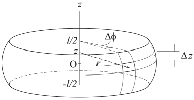
Figure 2: The strained cylindrical shell, showing schematically an elementary sector defined by the coordinates $r$, $\phi$ and $z$ ($\phi$ is implicit), and by the variations $\Delta\phi$ and $\Delta z$.

The equilibrium equations are derived from the analysis of the forces operating on an elementary sector of the shell, schematically represented in Fig. 2. The method is preferred over simply writing the equations of the theory of elasticity and applying boundary conditions because is simpler and provides better physical insight. The advantages of the procedure are discussed in the final subsection of this section.

Fig. 3 displays a diagram of the material element and the forces applied on it. Forces in the plane $\phi=\text{constant}$, containing the $z$–axis, are compressive forces of strength $F_{c}(z+\Delta z)$ and $F_{c}(z)$. The forces in the plane $z=\text{constant}$, normal to the $z$–axis, are tensile forces because stretch the shell contour in its plane, and their strength is denoted $F_{\phi}(z)$. Solutions with cylindrical symmetry were implicitly assumed because no dependence of the forces on $\phi$ was considered.

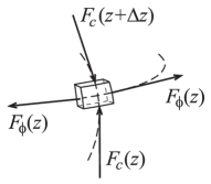
Figure 3: The elementary sector of Fig. 2 and the compressive and tensile forces $F_{c}$ and $F_{\phi}$ exerted on it.

Fig. 4(a) is a projection on the plane $z=\text{constant}$ of the system of Fig. 3 showing the forces operating in this plane, and Fig. 4(b) shows the vector composition of them. Hence, the tensile forces give a sum of strength

$$2F_{\phi}(z)\,\sin(\Delta\phi/2)\rightarrow F_{\phi}(z)\Delta\phi\;\,\text{if}\;\,\Delta\phi\approx 0,$$ (1)

contained in the plane $z=\text{constant}$ and pointing towards the central $z$–axis.

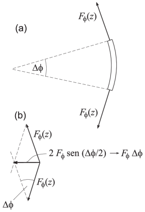
Figure 4: (a) The graphic scheme of Fig. 3 projected on the plane $z=\text{constant}$. (b) Force diagram in the plane $z=\text{constant}$.

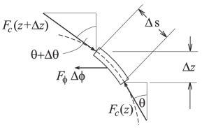
Figure 5: Forces in the plane $\phi=\text{constant}$. Compressive forces $F_{c}(z+\Delta z)$ and $F_{c}(z)$ are tangent to the curve $r(z)-R$ representing the shell profile, and subtend angles $\theta+\Delta\theta$ and $\theta$ with the $z$–axis, respectively. The force $F_{\phi}(z)\Delta\phi$ is obtained in Fig. 4 from the tensile forces in the plane $z=\text{constant}$. The discontinuous line represents the shell profile.

Forces in the plane $\phi=\text{constant}$ are shown in Fig. 5. They are the two compresive forces of strength $F_{c}(z+\Delta z)$ and $F_{c}(z)$ operating in the two opposite edges, and the third one is the resultant of the tensile forces in the plane $z=\text{constant}$, whose strength is $F_{\phi}(z)\Delta\phi$. The former two forces are tangent to the curve $r(z)-R$ determining the shell profile in the corresponding application points, and subtend angles $\theta+\Delta\theta$ and $\theta$ with the $z$–axis, respectively.

Equilibrium demands

$$-F_{c}(z+\Delta z)\cos(\theta+\Delta\theta)+F_{c}(z)\cos\theta=0,$$ (2)

$$F_{c}(z+\Delta z)\,\sin(\theta+\Delta\theta)-F_{c}(z)\,\sin\theta=-F_{\phi}\Delta\phi.$$ (3)

From Eq. (2) one can infer that the $z$–component of the forces does not depend on $z$, and hence they can be identified with the external force $P\Delta\phi/(2\pi)$ applied on the edge of the shell fringe defined by $\Delta\phi$. The argument is graphically shown in Fig. 6 and yields

$$F_{c}(z+\Delta z)\cos(\theta+\Delta\theta)=F_{c}(z)\cos\theta=\frac{P}{2\pi}\Delta\phi.$$ (4)

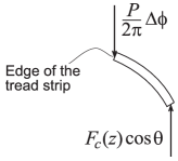
Figure 6: Equilibrium of a shell fringe of finite size in the $z$–direction. The $z$–component $F_{c}(z)\cos\theta$ of the force is $P\Delta\phi/(2\pi)$ for any $z$ in $[-l/2,l/2]$.

2.2 Differential equation for the shell profile function $r(z)-R$

Recalling Eqs. (4) one can divide the first term in the right hand side of Eq. (3) by $F_{c}(z+\Delta z)\cos(\theta+\Delta\theta)$, the second one by $F_{c}(z)\cos\theta$, and the right hand side by $P\Delta\phi/(2\pi)$. It gives

$$\tan(\theta+\Delta\theta)-\tan\theta=-\frac{2\pi F_{\phi}}{P}.$$ (5)

Force $F_{\phi}$ can be expressed as

$$F_{\phi}=\sigma_{\phi\phi}e\Delta s,$$ (6)

where $\sigma_{\phi\phi}$ is the normal stress in the azimuthal direction, $e$ is the shell thickness and $\Delta s$ the length of the shell element shown in Fig. 5, and whose value is

$$\Delta s=\sqrt{1+\left(\frac{dr}{dz}\right)^{2}}\,\Delta z.$$ (7)

.

Replacing $\tan\theta=dr/dz$ and combining Eqs. (5), (6) and (7) one obtains that, in the limit $\Delta z\rightarrow 0$,

$$\frac{d^{2}r}{dz^{2}}=-\frac{2\pi e\sigma_{\phi\phi}}{P}\sqrt{1+\left(\frac{dr}{dz}\right)^{2}}.$$ (8)

On the other hand, the normal stresses $\sigma_{rr}$, $\sigma_{\phi\phi}$ and $\sigma_{zz}$ satisfy Hooke’s law

$$\varepsilon_{\phi\phi}=\frac{r-R}{R}=\frac{1}{E}(\sigma_{\phi\phi}-\nu\sigma_{rr}-\nu\sigma_{zz}),$$ (9)

where $E$ and $\nu$ are the Young coefficient and Poisson ratio of the material the shell is made of. Substituting

$$\sigma_{zz}=-\frac{P}{2\pi re}\cos\theta,$$ (10)

$\cos\theta=[1+(dr/dz)^{2}]^{-1/2}$ and

$$\sigma_{rr}=-\frac{F_{\phi}\Delta\phi}{r\Delta\phi\Delta z}=-\sigma_{\phi\phi}\frac{e}{r}\sqrt{1+\bigg{(}\frac{dr}{dz}\bigg{)}^{2}}$$ (11)

in Eq. (9), and solving for $\sigma_{\phi\phi}$, it is obtained that

$$\sigma_{\phi\phi}=\frac{1}{1+\nu\dfrac{e}{r}\sqrt{1+\bigg{(}\dfrac{dr}{dz}\bigg{)}^{2}}}\left(E\,\frac{r-R}{R}-\frac{\nu P}{2\pi er\sqrt{1+\bigg{(}\dfrac{dr}{dz}\bigg{)}^{2}}}\right).$$ (12)

Combining Eqs. (12) and (8) one finally obtains

$$\frac{d^{2}r}{dz^{2}}=-\dfrac{\dfrac{2\pi eE}{RP}(r-R)\sqrt{1+\bigg{(}\dfrac{dr}{dz}\bigg{)}^{2}}-\dfrac{\nu}{r}}{1+\nu\dfrac{e}{r}\sqrt{1+\bigg{(}\dfrac{dr}{dz}\bigg{)}^{2}}}\,.$$ (13)

The differential equation (13) gives the profile $r(z)$ of the cylindrical shell deformed by the axial load $P$ when the proper physical conditions are imposed to the solutions. The most evident conclusion one can infer from Eq. (13) is that the load $P$ cannot be null. Hence it corresponds to a deformation regime occurring for high enough loads.

The unloaded cylindrical shell has a length $L$ in the axial direction, which reduces to a smaller length $l$ by the applied load $P$. The length reduction originates from the elastic compressive strain of the deformed mantle and by the shape deformation itself projected in the $z$–direction. If the elastic strain can be neglected when compared with the effect of the shell deformation, the length of the curved path adopted by the deformed shell will conserve its original value $L$. Hence the physical solutions of Eq. (13) must satisfy

$$L=\int_{-l/2}^{l/2}dz\,\sqrt{1+\left(\frac{dr}{dz}\right)^{2}}.$$ (14)

2.3 Present theoretical approach versus theory of elasticity

The equation for the shell profile was derived in the preceding subsections from analysing the equilibrium of the forces exerted on a representative elementary sector of the material medium, introducing from the beginning the symmetry constraints. For our present purposes, this procedure is much simpler and practical than the more standard approach of readily introducing the system boundary conditions into the general formalism of the theory of elasticity. This is because the latter approach oblige us to face complex problems we are not interested in. In the theory of elasticity the free surfaces of the shell are defined as surfaces where the stresses vanish, and the theory furnishes the equations for calculating the detailed structure of the stresses occurring in between. A recent paper by Zozulya and Zhang [8] provides a good example of this kind of precise calculation of the deformation of cylindrical shells, together with a detailed account of the stress fields inside the material. The cost paid for such a complete solution is the introduction of numerical methods from the very start.

However, it is not necessary here to know about the precise profiles of the outer and inner surfaces of the shell, or how vary the stresses inside. The forces $F_{c}(z)$ and $F_{\phi}(z)$ in Fig. 3 account for the integrated effect of these stresses, and their equilibrium condition proves to be enough for determining the equation for the mean shell profile, which has the advantage of being closed–form.

3 The profile equation in the buckling regime of deformation and its solution

The trivial solution $r=\text{constant}$ reduces Eq. (13) to

$$E\frac{r-R}{R}=\nu\frac{P}{2\pi re}\qquad(r=\text{constant}),$$ (15)

which can be interpreted as the Poisson effect on the shell circular perimeter $2\pi r$ accompanying the homogeneous axial strain produced by the applied compressive stress $P/(2\pi re)$. This uniform solution, which is expected to be stable up to a critical load $P_{B}$, preserves the cylindrical shape and produces only small geometrical variations, even for big loads, because $E$ is usually very large (0.01–500 GPa). The buckled non trivial solutions of Eq. (13) involve much larger deformations. In the post–buckling regime $r$ assumes values in the interval $R<r\leq R+L/2$ when $l$ varies from $l=L$ to $l=0$. The second term $\nu/r$ in the numerator of the right hand side of Eq. (13) is comparable with the first one only when $|r-R|/R\ll 1$. As long as $r$ departs from $R$ beyond the range of the purely elastic distortions, the term $\nu/r$ becomes negligibly small when compared with the one proportional to $E$. Hence it is advisable to distinguish between elastic strains and geometric changes and write

$$\frac{d^{2}r}{dz^{2}}=-\frac{2\pi eE}{PR}(r-R)\sqrt{1+\left(\frac{dr}{dz}\right)^{2}}\quad\text{(buckling regime)}.$$ (16)

Ec. (16) also assumes a thin enough shell to neglect the second term in the denominator of the right hand side of Ec. (13). Although this non-linear equation is not listed in the specialized treatises on elliptic functions and integrals [9, 10], it will be shown next that its exact solution is a Jacobi elliptic sine function, which holds for any load and deformation state, including the limit in which the shell has been completely flattened by the applied force.

Defining

$$y(z)=r(z)-R,\quad p=\frac{2\pi eE}{PR},\quad R=\text{constant},$$ (17)

Eq. (16) reads

$$y^{\prime\prime}=-py\sqrt{1+y^{\prime 2}},$$ (18)

and the substitution

$$y(z)=\frac{1}{\sqrt{p}}\,u(\sqrt{p}\,z)$$ (19)

turns it into

$$u^{\prime\prime}=-u\sqrt{1+u^{\prime 2}}.$$ (20)

Multiplying both sides of this equation by $u^{\prime}$ yields the integrable form

$$\frac{u^{\prime\prime}u^{\prime}}{\sqrt{1+u^{\prime 2}}}=-uu^{\prime},$$ (21)

which can be solved to give

$$\sqrt{1+u^{\prime 2}}=-\frac{1}{2}u^{2}+\frac{1}{2}u_{0}^{2}+1,$$ (22)

where $u_{0}=u(0)$. Because of the symmetry with respect to the origin, $u(\sqrt{p}\,z)$ must have its maximum at $z=0$ and the integration constant was chosen so that $u^{\prime}(0)=0$. Denoting now

$$\zeta=\sqrt{p}\,z,\quad v(\zeta)=\frac{u(\zeta)}{u_{0}},\quad k^{2}=\frac{(u_{0}/2)^{2}}{1+(u_{0}/2)^{2}}\,,$$ (23)

Eq. (22) can be rewritten as

$$\frac{dv}{d\zeta}=\sqrt{(1-v^{2})\bigg{(}1+\frac{u_{0}^{2}}{4}-\frac{u_{0}^{2}}{4}\,v^{2}\bigg{)}}\,,$$ (24)

or

$$\sqrt{1-k^{2}}\,\frac{dv}{d\zeta}=\sqrt{(1-v^{2})(1-k^{2}v^{2})}\,.$$ (25)

Inverting this equation and integrating with respect to $v$ one has

$$\frac{1}{\sqrt{1-k^{2}}}(\zeta+\zeta_{1})=\int_{\displaystyle\,0}^{\displaystyle\,v}\frac{dv}{\sqrt{(1-v^{2})(1-k^{2}v^{2})}}=F(v,k),$$ (26)

where $F(v,k)$ is the incomplete elliptic integral of the first kind with modulus $k$, ($0\leq k\leq 1$) [9, 10], and $\zeta_{1}$ is an integration constant. The same symbol was used for the integration variable and the upper integration limit to simplify the notation.

The inverse function of the incomplete elliptic integral $F(v,k)$ is known as the Jacobi elliptic sine function sn. Hence Eq. (26) is equivalent to

$$v=\text{sn }\bigg{(}\frac{\zeta+\zeta_{1}}{\sqrt{1-k^{2}}}\,,k\bigg{)}=\text{sn }\bigg{(}\sqrt{\frac{p}{1-k^{2}}}\,(z+z_{1}),k\bigg{)}.$$ (27)

Function $\text{sn }(x,k)$ takes values in the interval $[-1,1]$ and is periodic in $x$ with period $4K(k)$, where $K(k)=F(1,k)$ is the complete elliptic integral of the first kind. Also, $\text{sn }(0,k)=\text{sn }(2K,k)=0$ and $\text{sn }(K,k)=1$. The Jacobi sine function is symmetric with respect to $x=K$ and has a maximum there.

Therefore, the solution satisfying the boundary conditions $y(\pm l/2)=0$ is such that

$$\sqrt{\frac{p}{1-k^{2}}}=\frac{2K(k)}{l}\quad\text{and}\quad z_{1}=\frac{l}{2}.$$ (28)

Taking $\sqrt{p}$ and $z_{1}$ from these equations, and recalling the third of Eqs. (23), which gives $u_{0}/2=k/\sqrt{1-k^{2}}$, one has that the profile of the buckled cylindrical shell is given by

$$y(z)=r(z)-R=\frac{k}{(1-k^{2})K(k)}\,\text{sn }\bigg{[}\frac{2K(k)}{l}\bigg{(}z+\frac{l}{2}\bigg{)},k\bigg{]}.$$ (29)

Combining the first Eq. (28) with the definition (17) of the constant $p$, a relation between the applied force $P$ and $k$ follows

$$P=\frac{\pi eEl^{2}}{2R(1-k^{2})K^{2}(k)}.$$ (30)

Therefore, it rests just to determine the meaning of $k$ to have a complete solution of our problem. In the next subsection it will be shown that $k^{2}$ is essentially the relative axial deformation $\varepsilon=(L-l)/L$ of the cylindrical shell. The elliptic integral $K(k)$ can be calculated quite easily from the defining integral or the series

$$K(k)=\frac{\pi}{2}\bigg{[}1+\sum_{n=1}^{\infty}\bigg{(}\frac{(2n-1)!!}{2^{n}n!}\bigg{)}^{2}k^{2n}\bigg{]}.$$ (31)

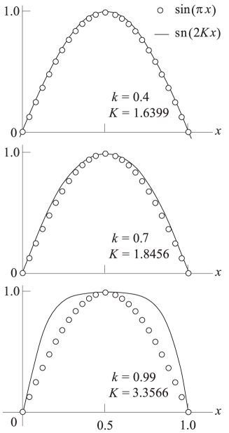
Figure 7: The Jacobi elliptic sine function (solid lines) for three values of the modulus $k$, compared with the trigonometric sine function (circles). For $k<0.7$ the two functions are very similar. At $k>0.7$ the elliptic function is sensibly broader and goes to a square wave in the limit $k=1$. Physically, $k=1$ corresponds to the situation in which the cylindrical mantle has been completely flattened by the applied force $P$ and $l=0$.

Fig. 7 shows the Jacobi sine function $\text{sn }(2Kx,k)$ for three values of $k$. The graphs makes apparent that the Jacobi elliptic function goes from $\sin(\pi x)$ to a square wave when the modulus $k$ goes from 0 to 1. The latter situation corresponds to the final collapse of the cylindrical mantle, when $l=0$.

3.1 The equation for the modulus $k$

When $R=\text{constant}$ one has $r^{\prime}(z)=y^{\prime}(z)=u^{\prime}(\sqrt{p}\,z)$, hence $(1+r^{\prime 2})^{1/2}$ can be replaced by $(1+u^{\prime 2})^{1/2}$ in the general condition expressed by Eq. (14). Making this and then substituting Eq. (22),

$$L=\int_{-l/2}^{l/2}\sqrt{1+u^{\prime 2}}\,dz=-\frac{1}{2}\int_{-l/2}^{l/2}u^{2}(\sqrt{p}\,z)\,dz+\frac{1}{2}u_{0}^{2}l+l.$$ (32)

Recalling now

$$u(\sqrt{p}\,z)=u_{0}\,\text{sn }\bigg{[}\frac{2K}{l}\bigg{(}z+\frac{l}{2}\bigg{)},k\bigg{]},\quad u_{0}=\frac{2k}{\sqrt{1+k^{2}}},$$ (33)

Eq. (32) can be written as

$$\frac{L-l}{l}=\frac{2k^{2}}{1-k^{2}}\left(1-\frac{1}{2K(k)}\int_{0}^{2K(k)}\text{ sn}^{2}\,(\zeta,k)\,d\zeta\right).$$ (34)

The integral appearing in this equation has been solved in terms of the elliptic functions and one has the mathematical identity [9]

$$\int\,\text{sn}^{2}\,\zeta\,d\zeta=\frac{1}{k^{2}}[u-E(\text{am }\zeta,k)],$$ (35)

where $E(\phi,k)$, $0\leq\phi\leq\pi/2$, is the second kind incomplete elliptic integral with modulus $k$. In the usual notation of the theory of elliptic integrals the amplitude am means $\text{am }\zeta=\arcsin(\text{sn }\zeta)$. Care must be taken in replacing properly the integration limits in the indefinite integral (35) because $0\leq\text{am }\zeta\leq\pi/2$, and $\text{am }K=\pi/2$. Therefore, $2K$ is outside the domain in which the amplitude function is defined. To overcome this difficulty one can take advantage of the symmetry of $\text{sn }(x,k)$ with respect to $x=K$ and write

$$\int_{0}^{2K}\,\text{sn}^{2}\,\zeta\,d\zeta=2\int_{0}^{K}\,\text{sn}^{2}\,\zeta\,d\zeta=\frac{2}{k^{2}}[K-E(\pi/2,k)]$$ (36)

replacing $\text{am }K=\pi/2$. $E(\pi/2,k)=E(k)$ is the complete elliptic integral of the second kind, modulus $k$, defined by the integral [9]

$$E(k)=\int_{0}^{\pi/2}\sqrt{1-k^{2}\sin^{2}\phi}\,d\phi,$$ (37)

or the series

$$E(k)=\frac{\pi}{2}\bigg{[}1-\sum_{n=1}^{\infty}\bigg{(}\frac{(2n-1)!!}{2^{n}n!}\bigg{)}^{2}\frac{k^{2n}}{2n+1}\bigg{]}.$$ (38)

The term $D(k)=(1/k^{2})[K(k)-E(k)]$ can be evaluated either by combining the power series (31) and (38) as

$$D(k)=\frac{K(k)-E(k)}{k^{2}}=\frac{\pi}{2}\sum_{n=0}^{\infty}\frac{2(n+1)}{2n+1}\bigg{(}\frac{(2n+1)!!}{2^{n+1}(n+1)!}\bigg{)}^{2}k^{2n},$$ (39)

or solving the integral

$$D(k)=\int_{0}^{\pi/2}\frac{\sin^{2}\phi\,d\phi}{\sqrt{1-k^{2}\sin^{2}\phi}}\,,$$ (40)

which follows directly from the definitions of $K(k)$ and $E(k)$.

Eq. (34) then becomes

$$\frac{\varepsilon}{1-\varepsilon}=\frac{2k^{2}}{1-k^{2}}\left(1-\frac{D(k)}{K(k)}\right),\quad\varepsilon=\frac{L-l}{L},$$ (41)

which determines exactly the modulus $k$ as a function of only the relative axial compression $\varepsilon=(L-l)/L$. The function $k=f(\varepsilon)$ does not depend on the characteristics of the cylindrical shell and is shown in Fig. 8. The amazingly simple approximate rule

$$k^{2}\approx\varepsilon$$ (42)

holds over the whole range of $\varepsilon$ with a 5% maximum error.

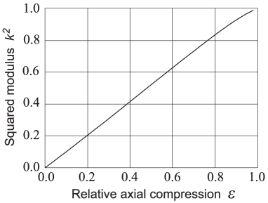
Figure 8: The squared modulus $k^{2}$ and the relative axial compression $\varepsilon=(L-l)/L$, as given by Eq. (41).

4 Critical load and reaction force

The deformation regime studied in the preceding sections takes place for a constant non–vanishing axial load $P$, given by Eq. (30). This is because it was assumed from the very beginning that loading curves the cylindrical shell profile and Eqs. (29), (30) and (41) hold at buckling and in the post–buckling regime of deformation. The variable $\varepsilon$ measures only the deformation induced relative displacement of the edges along the axial direction, and the much smaller elastic distortions have been neglected. The force

$$P=\frac{\pi eEL^{2}(1-\varepsilon)^{2}}{2R(1-k^{2})K^{2}(k)}$$ (43)

has an absolute maximum $P_{B}$ at $\varepsilon=k=0$. Recalling $K(0)=\pi/2$, the maximal reaction force reads

$$P_{B}=\frac{2eEL^{2}}{\pi R},$$ (44)

and one can write

$$\frac{P(\varepsilon)}{P_{B}}=\frac{\pi^{2}}{4}\frac{(1-\varepsilon)^{2}}{(1-k^{2})K^{2}(k)}.$$ (45)

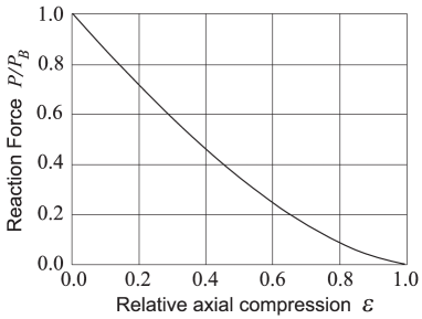
Figure 9: Reaction force $P$ relative to the maximum $P_{B}$ as a function of axial compression $\varepsilon=(L-l)/L$ , as given by Eq. (45).

Fig. 9 shows $P/P_{B}$, which according to Eqs. (45) and (41) is an universal function of $\varepsilon$. Fig. 10 displays the energy stored by the shell in the post–buckling deformation regime, obtained integrating Eq. (45) with respect to $\varepsilon$.

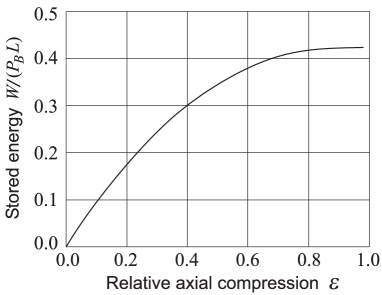
Figure 10: Energy absorbed by the cylindrical shell in the post–buckling deformation regime, in units of $P_{B}L$ and for any relative axial compression $\varepsilon$.

5 Homogeneous and buckled deformation regimes

The problem we are interested in is a deformation in which the cylindrical shell is gradually compressed along its main symmetry axis. In a first stage the compression is elastic and conserves the cylindrical shape. The relative displacement $x$ of the edges is given by Hookes’s law

$$\frac{P}{2\pi Re}=E\frac{x}{L_{0}},$$ (46)

where $L_{0}$ is the original length of the unstrained cylinder. Once the elastic distortion $x$ takes a critical value $x_{B}$, such that the applied force $P$ reaches the threshold strength $P_{B}$, the cylinder buckles and Eq. (43) starts holding, instead of Eq. (46). At the critical deformation $x_{B}$ the surface just starts to acquire the barrel shape, the two deformation regimes coexist and Eqs. (43) and (46) are both valid for $L=L_{0}-x_{B}$ and $\varepsilon=0$ (notice that $L$ stands for the the shell length when buckling is just initiated). Thus the axial deformation $x_{B}$ at which the buckling regime sets in can be obtained from combining Eqs. (44) and (46) to eliminate $P_{B}$. This yields

$$\frac{x_{B}}{L_{0}}=1+\left(\frac{\pi R}{\sqrt{2}L_{0}}\right)^{2}-\frac{\pi R}{\sqrt{2}L_{0}}\sqrt{\left(\frac{\pi R}{\sqrt{2}L_{0}}\right)^{2}+2},$$ (47)

which is the equation for the critical elastic strain $x_{B}/L_{0}$. The critical load is

$$P_{B}=2\pi ReE\,\bigg{[}1+\left(\frac{\pi R}{\sqrt{2}L_{0}}\right)^{2}-\frac{\pi R}{\sqrt{2}L_{0}}\sqrt{\left(\frac{\pi R}{\sqrt{2}L_{0}}\right)^{2}+2}\bigg{]}.$$ (48)

6 Conclusions relative to the marine application

To illustrate why vehicle old tires are functional as dock dampers in the light of the preceding equations, consider a 27”$\times$ 47” tire, originally designed for heavy mining trucks. The dimensions of the tread are $L_{0}=0.75\,\text{m}$, $R=1.25\,\text{m}$ and $e=0.10\,\text{m}$. Young’s effective modulus for tire rubber with added reinforcements can be estimated as $E=10\text{ MPa}$. The purpose of this calculation is fundamentally illustrative, to acquire a feeling of the magnitudes involved. Replacing these constants in Eqs. (47) and (48) one has that

$$x_{B}=2.55\,\text{cm}\quad P_{B}=267\,\text{kN}=27.3\,\text{ton}.$$ (49)

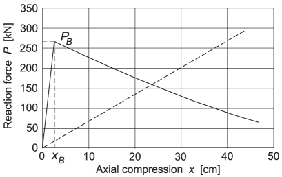
Figure 11: Axial reaction force $P$ exerted by a tire with tread dimensions $L_{0}=0.75\,\text{m}$, $R=1.25\,\text{m}$ and $e=0.10\,\text{m}$, and effective Young’s modulus $E=10\,\text{MPa}$, as a function of the axial compression $x$. The broken line shows the behaviour of a spring or any other strictly elastic medium chosen to yield a maximum force comparable with the tire.

Thus, when the tire is progresively compressed, the reaction force grows linearly with strain up to the critical strength $P_{B}=267\,\text{kN}$ at $x_{B}=2.55\,\text{cm}$, with the tread conserving its cylindrical shape. As compression continues, the tread curves and the radius turns dependent on $z$ according to Eq. (29). Fig. 11 shows the behaviour of the reaction $P$ of the strained tire in the two regimes, the linear and the buckled one (solid line). In the latter regime force $P$ obeys Eq. (45) with $L=L_{0}-x_{B}$. The broken line is the force exerted by a strictly elastic system, like a spring matrix, introduced here for the sake of comparison.

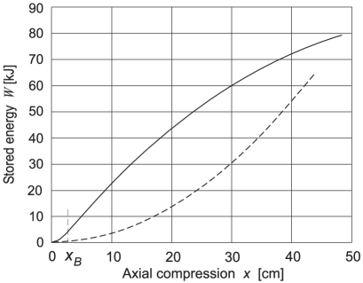
Figure 12: The solid curve represents the energy absorbed by the tire of Fig. 11 when compressed in a distance $x$. The broken curve is the same magnitude for the strictly elastic system. The smaller capacity of the latter for compressions in the range between 0 and 40 cm is apparent.

The stopping power of the tire when used as a dock bumper device is given by the area $W(x)$ under the curve of the reaction force. The solid line in Fig. 12 shows the curve of the energy stored $W(x)$ by the tire as a function of the compressive displacement $x$. The broken line displays the same magnitude for the purely elastic shock energy absorber.

Figs. 11 and 12 show the features that make tires good dock bumpers:
(a) The reaction force has a well defined maximum $P_{B}$, which ensures that the energy absorption device will not damage the colliding structures.
(b) Once the maximum reaction is reached, the reaction $P$ decreases smoothly with the displacement $x$, and energy storage $W(x)$ keeps high. This is the physical magnitude determining the stopping power of the device.
(c) Function $W(x)$ increases monotonically and rapidly with $x$, particularly for small values of $x$. This means that the stopping action of the axially compressed tire rapidly increases and keeps high at any strain, even for small ones. The superiority of the cylindrical shell (solid line) over a strictly elastic system (broken line) is shown quite dramatically in Fig. 12. The latter reaches an acceptable stopping ability at the cost of increasing the reaction force to a dangerous level.
(d) As $x$ takes relatively large values, the reaction force $P$ of the cylindrical bumper decreases to a fraction of its initial strength, reducing this way its ability to produce rebound. The elastic bumper produces the opposite effect.

Think for instance of a ship of mass $m=55,500\,\text{ton}$ being pushed by the tugs to approach normally the dock at a speed $v=0.24\,\text{knot}=0.1234\,\text{m/s}$ (a rather high speed). The kinetic energy of the ship is then $423\,\text{kJ}$. Assuming a safe tire compression of 0.4 m, the graph in Fig. 12 shows that each tire can store $W(0.40\,\text{m})=72.5\,\text{kJ}$, and then a minimum of six units would be necessary for safely docking the vessel. On the other hand, the ship side is specified to support a maximal load of $147\,\text{kN/m}^{2}$. The peak pressure the tires can exert on the ship side is $P_{B}/(\pi R^{2})=54.4\,\text{kN/m}^{2}$, which is close to 1/3 the specified maximum.

References

- [1] Young, W., Budynas, R.G., Budynas, R., Sadegh, A.: Roark’s Formulas for Stress and Strain, 8th. edition. McGraw–Hill, New York (2011).
- [2] Teng, J.G.: Buckling of thin shells: Recent advances and trends. Appl. Mech. Rev. 49 263–274 (1996).
- [3] Hunt, G.W., Lord, G.J., Peletier, M.A.: Cylindrical shell buckling: a characterization of localization and periodicity. Discrete and Continuous Dynamical Systems–Series B 4 505–518 (2003).
- [4] Paschero, M., Hyer, M.W.: Axial buckling of an orthotropic circular cylinder: Application to orthogrid concept. Int. J. Sol. Structures 46 2151–2171 (2009).
- [5] Pinna, R., Ronalds, B.F.: Buckling and postbuckling of cylindrical shells with one end pinned and the other end free. Thin-Walled Structures 41 507-527 (2003).
- [6] Simitses, G.J.: Buckling and postbuckling of imperfect cylindrical shells: A rewiew. Appl. Mech. Rev. 39 1517–1524 (1986).
- [7] Wullschleger, L., Meyer-Piening, H. R.: Buckling of geometrically imperfect cylindrical shells–definition of a buckling load. Int. J. Non-Linear Mech. 37 645–657 (2002).
- [8] Zozulya, V.V., Zhang, Ch.: A high order theory for functionally graded axisymmetric cylindrical shells. Int. J. Mech. Sci. 60 12 22 (2012).
- [9] Gradshteyn, I.S., Ryzhik, I.M.: Table of Integrals, Series, and Products, 7th edition. Academic Press, Burlington–San Diego–London (2007).
- [10] Byrd, P.F., Friedman, M. D.: Handbook of Elliptic Integrals for Engineers and Scientists, 2nd edition. Springer–Verlag, New York–Heidelberg–Berlin (1971).