Branching fraction measurement of $B^{+}\rightarrow\omega\ell^{+}\nu$ decays

Abstract

We present a measurement of the $B^{+}\rightarrow\omega\ell^{+}\nu$ branching fraction based on a sample of 467 million $B\kern 1.79993pt\overline{\kern-1.79993ptB}{}$ pairs recorded by the BABAR detector at the SLAC PEP-II $e^{+}e^{-}$ collider. We observe $1125\pm 131$ signal decays, corresponding to a branching fraction of ${\cal B}(B^{+}\rightarrow\omega\ell^{+}\nu)=(1.21\pm 0.14\pm 0.08)\times 10^{-4}$, where the first error is statistical and the second is systematic. The dependence of the decay rate on $q^{2}$, the invariant mass squared of the leptons, is compared to QCD predictions of the form factors based on a quark model and light-cone sum rules.

I Introduction

Most theoretical and experimental studies of exclusive $B\rightarrow X_{u}\ell\nu$ decays have focused on $B\rightarrow\pi\ell\nu$ decays, while $B\rightarrow\rho\ell\nu$ and $B^{+}\rightarrow\omega\ell^{+}\nu$ chg decays involving the vector mesons $\rho$ and $\omega$ have received less attention. Here $\ell$ is an electron or muon, and $X$ refers to a hadronic state, with the subscript $c$ or $u$ signifying whether the state carries charm or is charmless. Measurements of the branching fraction of $B\rightarrow\rho\ell\nu$ are impacted by an irreducible $B\rightarrow X_{u}\ell\nu$ background, typically the dominant source of systematic uncertainty. In studies of $B^{+}\rightarrow\omega\ell^{+}\nu$ that background can be suppressed to a larger degree, since the $\omega$ width is about 15 times smaller than that of the $\rho$. Extractions of the CKM matrix element $|V_{ub}|$ from $B^{+}\rightarrow\omega\ell^{+}\nu$ and $B\rightarrow\rho\ell\nu$ decay rates have greater uncertainties than those from $B\rightarrow\pi\ell\nu$, due to higher backgrounds and more complex form-factor dependencies. The persistent discrepancy between $|V_{ub}|$ measurements based on inclusive and exclusive charmless decays is a motivation for the study of different exclusive $B\rightarrow X_{u}\ell\nu$ decays J. Beringer et al. (2012); D. Asner et al. (2010).

Measurements of $\cal B$($B^{+}\rightarrow\omega\ell^{+}\nu$) have been reported by Belle C. Schwanda et al. (2004); I. Adachi et al. (2008); a measurement by BABAR has been performed on a partial dataset B. Aubert et al. (2009). In this analysis we use the full BABAR dataset to measure the total branching fraction $\cal B$($B^{+}\rightarrow\omega\ell^{+}\nu$) and partial branching fractions $\Delta{\cal B}(B^{+}\rightarrow\omega\ell^{+}\nu)/\Delta q^{2}$ in five $q^{2}$ intervals, where $q^{2}$ refers to the momentum transfer squared to the lepton system.

The differential decay rate for $B^{+}\rightarrow\omega\ell^{+}\nu$ is given by Richman and Burchat (1995)

$$\frac{{\rm d}\Gamma(B^{+}\rightarrow\omega\ell^{+}\nu)}{{\rm d}q^{2}}=|V_{ub}|^{2}\,\frac{G^{2}_{F}\,q^{2}\,p_{\omega}}{96\pi^{3}m_{B}^{2}c_{V}^{2}}$$

$$\times{}\bigg{[}|H_{0}|^{2}+|H_{+}|^{2}+|H_{-}|^{2}\bigg{]}\ ,$$ (1)

where $p_{\omega}$ is the magnitude of the $\omega$ momentum in the $B$ rest frame, $m_{B}$ is the $B$ mass, and $G_{F}$ is the Fermi coupling constant. The isospin factor $c_{V}$ is equal to $\sqrt{2}$ for $B^{+}\rightarrow\omega\ell^{+}\nu$ Ball and Zwicky (2005a). As described in a related BABAR paper P. del Amo Sanchez et al. (2011), the three helicity functions $H_{0}$, $H_{+}$, and $H_{-}$ can be expressed in terms of two axial vector form factors $A_{1}$ and $A_{2}$ and one vector form factor $V$, which describe strong interaction effects,

$$H_{\pm}(q^{2})=(m_{B}+m_{\omega})\bigg{[}A_{1}(q^{2})\mp\frac{2m_{B}\,p_{\omega}}{(m_{B}+m_{\omega})^{2}}V(q^{2})\bigg{]}\ ,$$

$$H_{0}(q^{2})=\frac{m_{B}+m_{\omega}}{2m_{\omega}\sqrt{q^{2}}}\times\bigg{[}(m_{B}^{2}-m_{\omega}^{2}-q^{2})A_{1}(q^{2})$$

$$-\frac{4m_{B}^{2}\,p_{\omega}^{2}}{(m_{B}+m_{\omega})^{2}}A_{2}(q^{2})\bigg{]}.$$

We compare the measured $q^{2}$ dependence of the decay rate with form factor predictions based on light-cone sum rules (LCSR) Ball and Zwicky (2005a) and the ISGW2 quark model Scora and Isgur (1995). We also use these form factor calculations and the measured branching fraction to extract $|V_{ub}|$.

II Detector, Data Set, and Simulation

The data used in this analysis were recorded with the BABAR detector at the PEP-II $e^{+}e^{-}$ collider operating at the $\mathchar 28935\relax{(4S)}$ resonance. We use a data sample of 426 $\mbox{\,fb}^{-1}$, corresponding to ($467\pm 5$) million produced $B\kern 1.79993pt\overline{\kern-1.79993ptB}{}$ pairs. In addition, we use 44 $\mbox{\,fb}^{-1}$ of data collected 40 $\mathrm{\,Me\kern-1.00006ptV}$ below the $B\kern 1.79993pt\overline{\kern-1.79993ptB}{}$ production threshold. This off-resonance sample is used to validate the simulation of the non-$B\kern 1.79993pt\overline{\kern-1.79993ptB}{}$ contributions whose principal source is $e^{+}e^{-}$ annihilation to $q\overline{q}$ pairs, where $q=u,d,s,c$.

The PEP-II collider and BABAR detector have been described in detail elsewhere B. Aubert et al. (2002a). Charged particles are reconstructed in a five-layer silicon tracker positioned close to the beam pipe and a forty-layer drift chamber. Particles of different masses are distinguished by their ionization energy loss in the tracking devices and by a ring-imaging Cerenkov detector. Electromagnetic showers from electrons and photons are measured in a finely segmented CsI(Tl) calorimeter. These detector components are embedded in a $1.5$ $\mathrm{T}$ magnetic field of a superconducting solenoid; its steel flux return is segmented and instrumented with planar resistive plate chambers and limited streamer tubes to detect muons that penetrate the magnet coil and steel.

We use Monte Carlo (MC) techniques Lange (2001); T. Sjöstrand (1994) to simulate the production and decay of $B\kern 1.79993pt\overline{\kern-1.79993ptB}{}$ and $q\overline{q}$ pairs and the detector response S. Agostinelli et al. (2003), to estimate signal and background efficiencies and resolutions, and to extract the expected signal and background distributions. The size of the simulated sample of generic $B\kern 1.79993pt\overline{\kern-1.79993ptB}{}$ events exceeds the $B\kern 1.79993pt\overline{\kern-1.79993ptB}{}$ data sample by about a factor of three, while the MC samples for inclusive and exclusive $B\rightarrow X_{u}\ell\nu$ decays exceed the data samples by factors of 15 or more. The MC sample for $q\overline{q}$ events is about twice the size of the $q\overline{q}$ contribution in the $\mathchar 28935\relax{(4S)}$ data.

The MC simulation of semileptonic decays uses the same models as in a recent BABAR analysis P. del Amo Sanchez et al. (2011). The simulation of inclusive charmless semileptonic decays $B\rightarrow X_{u}\ell\nu$ is based on predictions of a heavy quark expansion Fazio and Neubert (1999) for the differential decay rates. For the simulation of $B\rightarrow\pi\ell\nu$ decays we use the ansatz of Becirevic and Kaidalov (2000) for the $q^{2}$ dependence, with the single parameter $\alpha_{BK}$ set to the value determined in a previous BABAR analysis B. Aubert et al. (2007). All other exclusive charmless semileptonic decays $B\rightarrow X_{u}\ell\nu$, including the signal, are generated with form factors determined by LCSR Ball and Zwicky (2005a, b). For $B\rightarrow D\ell\nu$ and $B\rightarrow D^{*}\ell\nu$ decays we use parameterizations of the form factors Isgur and Wise (1989); I. Caprini and Neubert (1998) based on heavy quark effective theory; for the generation of the decays $B\rightarrow D^{**}\ell\nu$, we use the ISGW2 model Scora and Isgur (1995).

III Candidate Selection

In the following, we describe the selection and kinematic reconstruction of signal candidates, the definition of the various background classes, and the application of neural networks to further suppress these backgrounds.

The primary challenge in studying charmless semileptonic $B$ decays is to separate signal decays from Cabibbo-favored $B\rightarrow X_{c}\ell\nu$ decays, which have a branching fraction approximately 50 times larger than that of $B\rightarrow X_{u}\ell\nu$. A significant background also arises due to multi-hadron continuum events.

Based on the origin of the candidate lepton we distinguish three categories of events: 1) Signal candidates with a charged lepton from a true $B^{+}\rightarrow\omega\ell^{+}\nu$ decay; 2) $B\kern 1.79993pt\overline{\kern-1.79993ptB}{}$ background with a charged lepton from all non-signal $B\kern 1.79993pt\overline{\kern-1.79993ptB}{}$ events; 3) Continuum background from $e^{+}e^{-}\rightarrow q\bar{q}$ events. The $\omega$ meson is reconstructed in its dominant decay, $\omega\rightarrow\pi^{+}\pi^{-}\pi^{0}$. For each of the three categories of events we distinguish correctly reconstructed $\omega\rightarrow\pi^{+}\pi^{-}\pi^{0}$ decays (true-$\omega$) from combinatorial-$\omega$ candidates, for which at least one of the reconstructed pions originates from a particle other than the $\omega$.

III.1 Preselection

Signal candidates are selected from events with at least four charged tracks, since a $B^{+}\rightarrow\omega\ell^{+}\nu$ decay leaves three tracks and the second $B$ in the event is expected to produce at least one track. The magnitude of the sum of the charges of all reconstructed tracks is required to be less than two, helping to reject events with at least two undetected particles.

The preselection places requirements on the reconstructed lepton, $\omega$ meson, and neutrino from the $B^{+}\rightarrow\omega\ell^{+}\nu$ decay. At this stage in the analysis we allow for more than one candidate per event.

The lepton is identified as either an electron or muon. The electron identification efficiency is greater than 90% and constant as a function of momentum above 1 $\mathrm{\,Ge\kern-1.00006ptV}$, while the muon identification efficiency is between 65%–75% for momenta of 1.5–3 $\mathrm{\,Ge\kern-1.00006ptV}$. The pion misidentification rates are about 0.1% for the electron selector and 1% for the muon selector. The lepton is required to have a momentum in the center-of-mass (c.m.) frame greater than 1.6 $\mathrm{\,Ge\kern-1.00006ptV}$. This requirement significantly reduces the background from hadrons that are misidentified as leptons, and also removes a large fraction of true leptons from secondary decays or photon conversions and from $B\rightarrow X_{c}\ell\nu$ decays. The acceptance of the detector for leptons covers momentum polar angles in the range $0.41\leq\theta\leq 2.54\rm\,rad$.

For the reconstruction of the decay $\omega\rightarrow\pi^{+}\pi^{-}\pi^{0}$, we require that the candidate charged pions are not identified as leptons or kaons. The reconstructed $\omega$ mass must be in the range $680<m_{3\pi}<860\mathrm{\,Me\kern-1.00006ptV}$, and the $\pi^{0}$ candidate is required to have an invariant mass of $115<m_{\gamma\gamma}<150\mathrm{\,Me\kern-1.00006ptV}$. To reduce combinatorial $\omega$ background, we require minimum momenta for the three pion candidates, $p_{\pi^{\pm}}>200$ $\mathrm{\,Me\kern-1.00006ptV}$ and $p_{\pi^{0}}>400$ $\mathrm{\,Me\kern-1.00006ptV}$, and also energies of at least 80 $\mathrm{\,Me\kern-1.00006ptV}$ for photons from the $\pi^{0}$ candidate.

The charged lepton candidate is combined with an $\omega$ candidate to form a so-called $Y$ candidate. The charged tracks associated with the $Y$ candidate are fitted to a common vertex $Y_{\rm vtx}$. This vertex fit must yield a $\chi^{2}$ probability Prob$(\chi^{2},Y_{\rm vtx})>0.1$. To further reduce backgrounds without significant signal losses, we impose two-dimensional restrictions on the momenta of the lepton and $\omega$. Each $Y$ candidate must satisfy at least one of the following conditions on the c.m. momentum of the lepton and $\omega$: $p^{*}_{\omega}>1.3\mathrm{\,Ge\kern-1.00006ptV}$, or $p^{*}_{\ell}>2.0\mathrm{\,Ge\kern-1.00006ptV}$, or $p^{*}_{\ell}+p^{*}_{\omega}>2.65\mathrm{\,Ge\kern-1.00006ptV}$, where quantities with an asterisk refer to the c.m. frame. These requirements reject background candidates that are inconsistent with the phase space of the signal decay. The condition $|\cos\theta_{\rm BY}|\leq 1.0$, where $\cos\theta_{\rm BY}=(2E^{*}_{B}E^{*}_{Y}-M_{B}^{2}-M_{Y}^{2})/(2p^{*}_{B}\ p^{*}_{Y})$ is the cosine of the angle between the momentum vectors of the $B$ meson and the $Y$ candidate, should be fulfilled for a well-reconstructed $Y$ candidate originating from a signal decay B. H. Behrens et al. (2000). The energy $E^{*}_{B}$ and momentum $p^{*}_{B}$ of the $B$ meson are not measured event by event. Specifically, $E^{*}_{B}=\sqrt{s}/2$, where ${\sqrt{s}}$ is the c.m. energy of the colliding beams, and the $B$ momentum is derived as $p^{*}_{B}=\sqrt{E^{*2}_{B}-m^{2}_{B}}$. To allow for the finite resolution of the detector, we impose the requirement $-1.2<\cos\theta_{\rm BY}<1.1$.

The neutrino four-momentum is inferred from the missing energy and momentum of the whole event: $(E_{\rm miss},\vec{p}_{\rm miss})=(E_{e^{+}e^{-}},\vec{p}_{e^{+}e^{-}})-(\sum_{i}{E_{i}},\sum_{i}{\vec{p}_{i}})$, where $E_{e^{+}e^{-}}$ and $\vec{p}_{e^{+}e^{-}}$ are the energy and momentum of the colliding beam particles, and the sums are performed over all tracks and all calorimeter clusters without an associated track. If all tracks and clusters in an event are well-measured, and there are no undetected particles besides a single neutrino, then the measured distribution of the missing mass squared, $m^{2}_{\rm miss}=E_{\rm miss}^{2}-{p}_{\rm miss}^{2}$, peaks at zero. We require the reconstructed neutrino mass to be consistent with zero, $|m_{\rm miss}^{2}/(2E_{\rm miss})|<2.5\mathrm{\,Ge\kern-1.00006ptV}$, and the missing momentum to exceed 0.5 $\mathrm{\,Ge\kern-1.00006ptV}$. The polar angle of the missing momentum vector is also required to pass through the fiducial region of the detector, $0.3<\theta_{\rm miss}<2.2\rm\,rad$.

Other restrictions are applied to suppress $q\bar{q}$ background, which has a two-jet topology in contrast to $B\kern 1.79993pt\overline{\kern-1.79993ptB}{}$ events with a more uniform angular distribution of the tracks and clusters. Events must have $R_{2}\leq 0.5$, where $R_{2}$ is the second normalized Fox-Wolfram moment Fox and Wolfram (1979), determined from all charged and neutral particles in the event. We also require $\cos\Delta\theta_{\rm thrust}\leq 0.9$, where $\Delta\theta_{\rm thrust}$ is the angle between the thrust axis of the $Y$ candidate’s decay particles and the thrust axis of all other detected particles in the event. We require $L_{2}<3.0\mathrm{\,Ge\kern-1.00006ptV}$, with $L_{2}=\sum_{i}p^{*}_{i}{\cos}^{2}\theta^{*}_{i}$, where the sum runs over all tracks in the event excluding the $Y$ candidate, and $p^{*}_{i}$ and $\theta^{*}_{i}$ refer to the c.m. momenta and the angles measured with respect to the thrust axis of the $Y$ candidate.

We reject candidates that have a charged lepton and a low-momentum charged pion consistent with a $B^{0}\rightarrow D^{*-}\ell^{+}\nu$, $D^{*-}\rightarrow\kern 1.99997pt\overline{\kern-1.99997ptD}{}^{0}\pi^{-}_{\rm slow}$ decay as described in B. Aubert et al. (2002b).

The kinematic consistency of the candidate decay with a signal $B$ decay is ascertained by restrictions on two variables, the beam-energy substituted $B$ mass $m_{\rm ES}$, and the difference between the reconstructed and expected energy of the $B$ candidate $\Delta E$. In the laboratory frame these variables are defined as $m_{\rm ES}=\sqrt{(s/2+\vec{p}_{B}\cdot\vec{p}_{e^{+}e^{-}})\,^{2}/E_{e^{+}e^{-}}^{2}-p_{B}^{2}}$ and $\Delta E=(P_{e^{+}e^{-}}\cdot P_{B}-s/2)/\sqrt{s}$, where $P_{B}=(E_{B},\vec{p}_{B})$ and $P_{e^{+}e^{-}}=(E_{e^{+}e^{-}},\vec{p}_{e^{+}e^{-}})$ are the four-momenta of the $B$ meson and the colliding beams, respectively. For correctly reconstructed signal $B$ decays, the $\Delta E$ distribution is centered at zero, and the $m_{\rm ES}$ distribution peaks at the $B$ mass. We restrict candidates to $-0.95<\Delta E<0.95\mathrm{\,Ge\kern-1.00006ptV}$ and $5.095<m_{\rm ES}<5.295\mathrm{\,Ge\kern-1.00006ptV}$.

III.2 Neural Network Selection

To separate signal candidates from the remaining background we employ two separate neural networks (NN), to suppress $q\bar{q}$ background and $B\rightarrow X_{c}\ell\nu$ background. The $q\bar{q}$ NN is trained on a sample passing the preselection criteria, while the $B\rightarrow X_{c}\ell\nu$ NN is trained on a sample passing both the preselection and the $q\bar{q}$ neural network criteria. The training is performed with signal and background MC samples. These NN are multilayer perceptrons that have two hidden layers with seven and three nodes.

The variables used as inputs to the $q\bar{q}$ NN are $R_{2}$, $L_{2}$, $\cos\Delta\theta_{\rm thrust}$, $\cos\theta_{\rm BY}$, $m_{\rm miss}^{2}/(2E_{\rm miss})$, Prob$(\chi^{2},Y_{\rm vtx})$, the polar angle of the missing momentum vector in the laboratory frame, and the Dalitz plot amplitude $A_{\rm Dalitz}=\alpha|{\vec{p}}_{\pi^{+}}\times{\vec{p}}_{\pi^{-}}|$, with the $\pi^{+}$ and $\pi^{-}$ momenta measured in the $\omega$ rest frame and scaled by a normalization factor $\alpha$. True $\omega$ mesons typically have larger values of $A_{\rm Dalitz}$ than combinatorial $\omega$ candidates reconstructed from unrelated pions. The $B\rightarrow X_{c}\ell\nu$ NN uses the same variables, except for $\cos\Delta\theta_{\rm thrust}$, which is replaced by $\cos\theta_{W\ell}$, the helicity angle of the lepton, defined as the angle between the momentum of the lepton in the rest frame of the virtual $W$ and the momentum of the $W$ in the rest frame of the $B$. The data and MC simulation agree well for the NN input variables at each stage of the selection. The NN discriminators are chosen by maximizing $\sqrt{\epsilon_{\rm sig}^{2}+(1-\eta_{\rm bkg})^{2}}$, where $\epsilon_{\rm sig}$ is the efficiency of the signal and $\eta_{\rm bkg}$ is the fraction of the background misidentified as signal.

The selection efficiencies for the various stages of the candidate selection for the signal and background components are given in Table 1. After the preselection and NN selection, 21% of events in data contribute multiple $B^{+}\rightarrow\omega\ell^{+}\nu$ candidates. The candidate with the largest value of Prob$(\chi^{2},Y_{\rm vtx})$ is retained. For the remaining candidates, the reconstructed 3-pion mass is required to be consistent with the $\omega$ nominal mass K. Nakamura et al. (2010), $|m_{3\pi}-m_{\omega}|<23\mathrm{\,Me\kern-1.00006ptV}$. The overall signal efficiency is 0.73% if the reconstructed candidate includes a true $\omega$ and 0.21% if it includes a combinatorial $\omega$. The efficiencies of the $B\kern 1.79993pt\overline{\kern-1.79993ptB}{}$ and $q\bar{q}$ backgrounds are suppressed by several orders of magnitude relative to the signal.

Table 1: Successive efficiencies (in %) predicted by MC simulation for each stage of the selection, for true- and combinatorial-$\omega$ signal, and backgrounds from $B\kern 1.79993pt\overline{\kern-1.79993ptB}{}$ and $q\bar{q}$ events.

Source	true-$\omega$	comb.-$\omega$	$B\kern 1.79993pt\overline{\kern-1.79993ptB}{}$	$q\bar{q}$
	signal	signal
Preselection	1.9	4.8	0.0094	0.00073
Neural nets	43	17	7.9	11
3-pion mass	88	26	24	30
Total (product)	0.73	0.21	0.00018	0.000024

III.3 Data-MC Comparisons

The determination of the number of signal events relies heavily on the MC simulation to correctly describe the efficiencies and resolutions, as well as the distributions for signal and background sources. Therefore a significant effort has been devoted to detailed comparisons of data and MC distributions, for samples that have been selected to enhance a given source of background.

Specifically, we have studied the MC simulation of the neutrino reconstruction for a control sample of $B^{0}\rightarrow D^{*-}\ell^{+}\nu$ decays, with $D^{*-}\rightarrow\kern 1.99997pt\overline{\kern-1.99997ptD}{}^{0}\pi_{\rm slow}^{-}$ and $\kern 1.99997pt\overline{\kern-1.99997ptD}{}^{0}\rightarrow K^{+}\pi^{-}\pi^{0}$. This final state is similar to that of the $B^{+}\rightarrow\omega\ell^{+}\nu$ decay, except for the addition of the slow pion $\pi_{s}^{-}$ and the substitution of a $K^{+}$ for a $\pi^{+}$. This control sample constitutes a high-statistics and high-purity sample on which to test the neutrino reconstruction. We compare data and MC distributions for the control sample and find good agreement for the variables used in the preselection and as inputs to the NN. We have also used this sample to study the resolution of the neutrino reconstruction and its impact on $q^{2}$, $m_{\rm ES}$, and $\Delta E$.

IV Signal Extraction

IV.1 Fit Method

We determine the signal yields by performing an extended binned maximum-likelihood fit to the observed three-dimensional $\Delta E$-$m_{\rm ES}$-$q^{2}$ distributions. The fit technique Barlow and Beeston (1993) accounts for the statistical fluctuations of the data and MC samples.

For this fit the $\Delta E$-$m_{\rm ES}$ plane is divided into 20 bins, as shown in Fig. 1, and the data are further subdivided into five bins in $q^{2}$, chosen to contain roughly equal numbers of signal events. The $q^{2}$ resolution is dominated by the neutrino reconstruction. It can be improved by substituting the missing energy with the magnitude of the missing momentum and by rescaling $\vec{p}_{\rm miss}$ to force $\Delta E=0$, $q^{2}_{\rm corr}={[(E_{\ell},\vec{p}_{\ell})+\delta\cdot(p_{\rm miss},\vec{p}_{\rm miss})]}^{2}$, where $\delta=1-\Delta E/E_{\rm miss}$. This correction to $q^{2}$ is used in the fit.

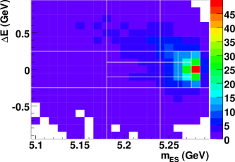
Figure 1: Distribution of $\Delta E$ versus $m_{\rm ES}$ for true-$\omega$ signal MC. The 20 bins into which the plane is divided for the fit histogram are overlaid.

We describe the measured $\Delta E$-$m_{\rm ES}$-$q^{2}$ distribution as a sum of four contributions: $B^{+}\rightarrow\omega\ell^{+}\nu$ signal (both true-$\omega$ and combinatoric-$\omega$), true-$\omega$ $B\kern 1.79993pt\overline{\kern-1.79993ptB}{}$, true-$\omega$ $q\bar{q}$, and the sum of the combinatorial-$\omega$ background from $B\kern 1.79993pt\overline{\kern-1.79993ptB}{}$ and $q\bar{q}$ events.

While the $\Delta E$-$m_{\rm ES}$ shapes for the signal and true-$\omega$ $B\kern 1.79993pt\overline{\kern-1.79993ptB}{}$ and $q\bar{q}$ sources are taken from MC samples, we choose to represent the dominant combinatorial-$\omega$ background by the distributions of data events in the $m_{3\pi}$ sidebands, thereby reducing the dependence on MC simulation of these backgrounds. The normalization of these background data is taken from a fit to the 3-$\pi$ mass distribution in the range $0.680<m_{3\pi}<0.880$ $\mathrm{\,Ge\kern-1.00006ptV}$. To obtain a sample corresponding to the combinatorial-$\omega$ background from $B\kern 1.79993pt\overline{\kern-1.79993ptB}{}$ and $q\bar{q}$ events only, we subtract the MC simulated $m_{3\pi}$ contribution of the small combinatorial-$\omega$ $B^{+}\rightarrow\omega\ell^{+}\nu$ signal sample. To the resulting $m_{3\pi}$ distribution we fit the sum of a relativistic Breit-Wigner convolved with a normalized Gaussian function, and the combinatorial background described by a second degree polynomial. The resulting fit to the $m_{3\pi}$ distribution for the all-$q^{2}$ sample is shown in Fig. 2. The $\chi^{2}$ per number of degrees of freedom (dof) for the fits are within the range expected for good fits. The fitted background function is used to determine the weights to apply to the upper and lower sidebands to scale them to the expected yield of combinatorial-$\omega$ $B\kern 1.79993pt\overline{\kern-1.79993ptB}{}$ and $q\bar{q}$ background in the $m_{3\pi}$ peak region.

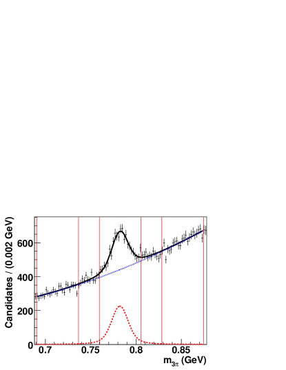
Figure 2: Fit to the distribution of $m_{3\pi}$ for data from the all-$q^{2}$ sample, with MC combinatorial-$\omega$ signal subtracted. The dashed (red) and dotted (blue) curves describe the fitted peaking and combinatorial background functions, respectively, and the solid (black) curve is their sum. The peak and sideband regions are also indicated.

The peak and two sideband regions are chosen to have a width of 46 $\mathrm{\,Me\kern-1.00006ptV}$ and are separated by 23 $\mathrm{\,Me\kern-1.00006ptV}$, as indicated in Fig. 2. Since the normalization of the combinatorial-$\omega$ signal contribution depends on the fitted signal yield, which is a priori unknown, this component is determined iteratively.

The fit has seven free parameters, five for the signal yields in each $q^{2}$ bin, and one each for the yields of the true-$\omega$ $B\kern 1.79993pt\overline{\kern-1.79993ptB}{}$ and $q\bar{q}$ backgrounds, the shapes of the distributions are taken from MC simulations. The fitted yields are expressed as scale factors relative to the default yields of the MC simulation. The total signal yield is taken as the sum of the fitted yields in the individual $q^{2}$ bins, taking into account correlations.

IV.2 Fit Results

Table 2: Number of events and their statistical uncertainties, as determined from the fit, compared with the number of observed events in data. The combinatorial-$\omega$ background yields are fixed in the fit; the quoted uncertainties are derived from the sideband subtraction.

$q^{2}$ range ($\rm\,Ge\kern-0.80002ptV^{2}$)	0–4	4–8	8–10	10–12	12–21	0–21
All signal	257 $\pm$ 72	238 $\pm$ 44	161 $\pm$ 32	177 $\pm$ 32	293 $\pm$ 57	1125 $\pm$ 131
True-$\omega$ signal	238	209	136	137	168	869
Comb.-$\omega$ signal	19	28	25	40	125	256
$B\kern 1.79993pt\overline{\kern-1.79993ptB}{}$ (true-$\omega$)	105 $\pm$ 19	192 $\pm$ 34	154 $\pm$ 27	195 $\pm$ 34	411 $\pm$ 73	1057 $\pm$ 187
$q\bar{q}$ (true-$\omega$)	409 $\pm$ 96	145 $\pm$ 34	65 $\pm$ 15	34 $\pm$ 8	64 $\pm$ 15	716 $\pm$ 167
Comb.-$\omega$ bkgd.	1741 $\pm$ 23	1818 $\pm$ 24	1240 $\pm$ 20	1520 $\pm$ 22	3913 $\pm$ 35	10232 $\pm$ 57
Data	2504 $\pm$ 50	2433 $\pm$ 49	1605 $\pm$ 40	1858 $\pm$ 43	4738 $\pm$ 69	13138 $\pm$ 115

The fitting procedure has been validated on pseudo-experiments generated from the MC distributions. We find no biases and the uncertainties follow the expected statistical distribution.

The yields of the signal, true-$\omega$ $B\kern 1.79993pt\overline{\kern-1.79993ptB}{}$, and true-$\omega$ $q\bar{q}$ components obtained from the binned maximum-likelihood fit to $\Delta E$-$m_{\rm ES}$-$q^{2}$ are presented in Table 2. Projections of the fitted distributions of $m_{\rm ES}$ for the all-$q^{2}$ fit and for the five $q^{2}$ bins fit are shown in Fig. 3. The agreement between the data and fitted MC samples is reasonable for distributions of $\Delta E$, $m_{\rm ES}$, and $q^{2}$, as indicated by the $\chi^{2}/{\rm dof}$ of the fit, 106/93, which has a probability of 16%. The fixed combinatorial-$\omega$ background yield accounts for 83% of all backgrounds. The correlations among the parameters are listed in Table 3. The strongest correlation is $-72\%$, between the signal and $q\bar{q}$ yields in the first $q^{2}$ bin, which contains most of the $q\bar{q}$ background. The correlation between signal and $B\kern 1.79993pt\overline{\kern-1.79993ptB}{}$ background is strongest in the last $q^{2}$ bin, $-40\%$, because of a large contribution from other $B\rightarrow X_{u}\ell\nu$ decays. Correlations among signal yields are significantly smaller.

Table 3: Correlations among the fit scale factors $p^{s}_{k}$ for the simulated source $s$ and $q^{2}$ bin $k$. The scale factors for $q\bar{q}$ and $B\kern 1.79993pt\overline{\kern-1.79993ptB}{}$ apply to the full $q^{2}$ range.

		$p^{q\bar{q}}$	$p^{B\kern 1.25995pt\overline{\kern-1.25995ptB}{}}$	$p_{1}^{\omega\ell\nu}$	$p_{2}^{\omega\ell\nu}$	$p_{3}^{\omega\ell\nu}$	$p_{4}^{\omega\ell\nu}$	$p_{5}^{\omega\ell\nu}$
	$p^{q\bar{q}}$	1.000	$-$0.466	$-$0.724	$-$0.106	$-$0.031	0.051	0.088
	$p^{B\kern 1.25995pt\overline{\kern-1.25995ptB}{}}$		1.000	0.223	$-$0.249	$-$0.253	$-$0.284	$-$0.401
	$p_{1}^{\omega\ell\nu}$			1.000	0.121	0.061	0.001	$-$0.011
	$p_{2}^{\omega\ell\nu}$				1.000	0.105	0.094	0.128
	$p_{3}^{\omega\ell\nu}$					1.000	0.088	0.121
	$p_{4}^{\omega\ell\nu}$						1.000	0.125
	$p_{5}^{\omega\ell\nu}$							1.000

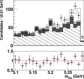
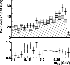
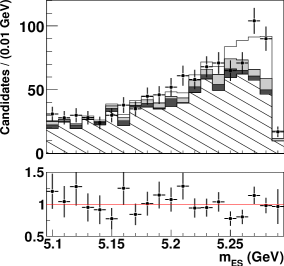
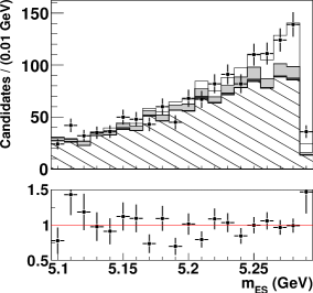
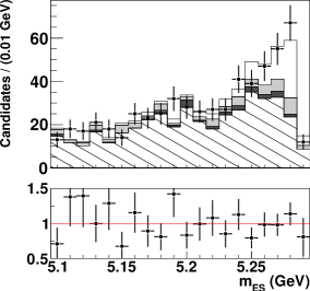
$0<q^{2}<4\rm\,Ge\kern-0.80002ptV^{2}$ $10<q^{2}<12\rm\,Ge\kern-0.80002ptV^{2}$ $4<q^{2}<8\rm\,Ge\kern-0.80002ptV^{2}$ $12<q^{2}<21\rm\,Ge\kern-0.80002ptV^{2}$ $8<q^{2}<10\rm\,Ge\kern-0.80002ptV^{2}$ $0<q^{2}<21\rm\,Ge\kern-0.80002ptV^{2}$

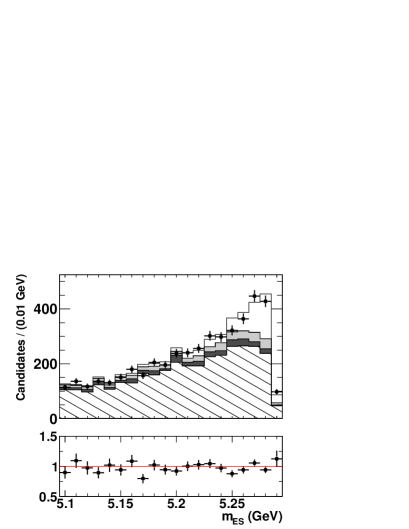
Figure 3: Distributions of $m_{\rm ES}$ after the fit and the ratio of the data to the fitted predictions, for five separate $q^{2}$ bins and the full $q^{2}$ range, in the $\Delta E$ signal band, $-0.25<\Delta E\leq 0.25\mathrm{\,Ge\kern-1.00006ptV}$. The points represent data with statistical uncertainties, while the stacked histograms represent the sum of fitted source components, signal (white), true-$\omega$ $B\kern 1.79993pt\overline{\kern-1.79993ptB}{}$ (light gray), true-$\omega$ $q\bar{q}$ (dark gray), and combinatorial-$\omega$ background (diagonally thatched).

The branching fraction, $\cal B$($B^{+}\rightarrow\omega\ell^{+}\nu$), averaged over electron and muon channels, is defined as ${\cal B}(B^{+}\rightarrow\omega\ell^{+}\nu)=\sum_{i}(N_{i}^{\mathrm{sig}}/\epsilon_{i}^{\mathrm{sig}})/(4f_{\pm}N_{B\kern 1.25995pt\overline{\kern-1.25995ptB}{}})$, where $N_{i}^{\rm sig}$ refers to the number of reconstructed electron and muon signal events in $q^{2}$ bin $i$, $\epsilon_{i}^{\rm sig}$ is the reconstruction efficiency, $f_{\pm}$ is the fraction of $B^{+}{\kern-1.60004ptB^{-}}$ decays in all $B\kern 1.79993pt\overline{\kern-1.79993ptB}{}$ events, and $N_{B\kern 1.25995pt\overline{\kern-1.25995ptB}{}}$ is the number of produced $B\kern 1.79993pt\overline{\kern-1.79993ptB}{}$ events. The factor of 4 comes from the fact that ${\cal B}$ is quoted as the average of $\ell=e$ and $\mu$ samples, not the sum, and the fact that either of the two $B$ mesons in the $B^{+}{\kern-1.60004ptB^{-}}$ event may decay into the signal mode. The $q^{2}$ resolution in the signal region is 0.36 $\rm\,Ge\kern-0.80002ptV^{2}$, smaller than the width of the $q^{2}$ bins. To account for the finite $q^{2}$ resolution, the background-subtracted, efficiency-corrected spectrum is adjusted by deriving from the signal MC the ratio of the true and reconstructed $q^{2}$ spectra, $({\rm d}{\cal B}/{\rm d}q^{2}_{\rm true})/({\rm d}{\cal B}/{\rm d}q^{2}_{\rm reco})$. This ratio differs by 9% at low $q^{2}$ and considerably less at higher $q^{2}$. The partial and total branching fractions listed in Table 4 are corrected for the effects of finite $q^{2}$ resolution and efficiency.

Table 4: Measured $B^{+}\rightarrow\omega\ell^{+}\nu$ branching fraction and partial branching fractions in bins of $q^{2}$ with statistical and systematic uncertainties.

$q^{2}$ ($\rm\,Ge\kern-0.80002ptV^{2}$)	$\Delta{\cal B}$ $(\times 10^{-4}$)
0–4	0.214 $\pm$ 0.060 $\pm$ 0.024
4–8	0.200 $\pm$ 0.037 $\pm$ 0.010
8–10	0.147 $\pm$ 0.029 $\pm$ 0.010
10–12	0.169 $\pm$ 0.031 $\pm$ 0.010
12–21	0.482 $\pm$ 0.093 $\pm$ 0.038
0–12	0.730 $\pm$ 0.083 $\pm$ 0.054
0–21	1.212 $\pm$ 0.140 $\pm$ 0.084

V Systematic Uncertainties

Table 5 summarizes the contributions to the systematic uncertainty. The event reconstruction systematic uncertainties are most sensitive to the neutrino reconstruction, which depends on the detection of all of the particles in the event. To assess the impact of the uncertainty of the measured efficiencies for charged tracks, the MC signal and background samples are reprocessed and the analysis is repeated, after tracks have been eliminated at random with a probability determined by the uncertainty in the tracking efficiency. Similarly, we evaluate the impact from uncertainties in the photon reconstruction efficiency by eliminating photons at random as a function of the photon energy. Since a $K^{0}_{\scriptscriptstyle L}$ leaves no track and deposits only a small fraction of its energy in the calorimeter, the reconstruction of the neutrino is impacted. The uncertainty on the $K^{0}_{\scriptscriptstyle L}$ MC simulation involves the shower energy deposited by the $K^{0}_{\scriptscriptstyle L}$ in the calorimeter, the $K^{0}_{\scriptscriptstyle L}$ detection efficiency, and the inclusive $K^{0}_{\scriptscriptstyle L}$ production rate as a function of momentum from $B\kern 1.79993pt\overline{\kern-1.79993ptB}{}$ events.

The impact of the changes to the simulated background distributions which enter the fit are smaller than for the signal, since the large combinatorial backgrounds are taken from data, rather than MC simulations. As an estimate of the impact of these variations of the MC simulated distributions on the $q^{2}$ dependent signal yield, we combine the observed reduction in the signal distribution with the impact of the changes to $q\bar{q}$ and $B\kern 1.79993pt\overline{\kern-1.79993ptB}{}$ backgrounds on the signal yield, taking into account the correlations obtained from the fit (see Table III). Since the correlations between signal and backgrounds are small at high $q^{2}$, the impact of the uncertainties in the background are also modest. This procedure avoids large statistical fluctuations of the fit procedure that have been observed to be larger than the changes in the detection efficiencies. However, this procedure does not account for the small changes in the shape of the distributions, and we therefore sum the magnitude of the changes for signal and background, rather than adding them in quadrature or taking into account the signs of the correlations of the signal and backgrounds in a given $q^{2}$ bin.

We assign an uncertainty on the identification efficiency of electrons and muons, as well as on the lepton and kaon vetoes of the $\omega$ daughter pions, based on the change in signal yield after varying the selector efficiencies within their uncertainties.

The uncertainty in the calculation of the LCSR form factors impacts the uncertainty on the branching fraction because it affects the predicted $q^{2}$ distribution of the signal and thereby the fitted signal yield. We assess the impact by varying the form factors within their uncertainties. We include the uncertainty on the branching fraction of the $\omega$ decay, $\cal B$($\omega$ $\rightarrow\pi^{+}\pi^{-}\pi^{0}$) = $(89.2\pm 0.7)\times 10^{-2}$ K. Nakamura et al. (2010). To evaluate the uncertainty from radiative corrections, candidates are reweighted by 20% of the difference between the spectra with and without PHOTOS Barberio and Was (1994), which models the final state radiation of the decay.

The uncertainty on the true-$\omega$ backgrounds has a small impact on the signal yield since these components represent a small fraction of the total sample. To assess the uncertainty of the $\Delta E$-$m_{\rm ES}$-$q^{2}$ shapes of the true-$\omega$ $q\bar{q}$ and true-$\omega$ $B\kern 1.79993pt\overline{\kern-1.79993ptB}{}$ samples, the fit is repeated after the events are reweighted to reproduce the inclusive $\omega$ momentum distribution measured in $B\kern 1.79993pt\overline{\kern-1.79993ptB}{}$ and $q\bar{q}$ events. We also assess the uncertainty on the modeling of the semileptonic backgrounds by varying the branching fractions and form factors of the exclusive and inclusive $B\rightarrow X_{u}\ell\nu$ K. Nakamura et al. (2010) and $B\rightarrow X_{c}\ell\nu$ backgrounds D. Asner et al. (2010) within their uncertainties.

To assess the uncertainties that result from the MC prediction of the $m_{3\pi}$ distribution of the combinatorial-$\omega$ signal, we use the uncorrected distribution, in which the combinatorial-$\omega$ signal is not subtracted from the $m_{3\pi}$ sidebands, and the signal fit parameter is set to scale only the true-$\omega$ signal contribution. Twenty percent of the difference between the nominal and uncorrected results is taken as the systematic uncertainty; it is largest for $12<q^{2}<21\rm\,Ge\kern-0.80002ptV^{2}$ because the fraction of combinatorial-$\omega$ signal in this $q^{2}$ bin is large. The sideband event yields determined from the $m_{3\pi}$ fit are varied within their fit errors to determine the statistical uncertainty on the combinatorial-$\omega$ background. The uncertainty in the chosen $m_{3\pi}$ ansatz is assessed by repeating the $m_{3\pi}$ fits, replacing the nominal functions for the peak and background components. For the background component, we use a third instead of a second degree polynomial. For the peaking component, we use a Gaussian function in place of a relativistic Breit-Wigner convoluted with a Gaussian function. The systematic error from the $m_{3\pi}$ ansatz is taken as the sum in quadrature of the change in signal yield for each of these functional variations.

The branching fraction depends inversely on the value of $N_{B\kern 1.25995pt\overline{\kern-1.25995ptB}{}}$, which is determined with a precision of $1.1\%$ McGregor (2008). At the $\mathchar 28935\relax{(4S)}$ resonance, the fraction of $B^{+}{\kern-1.60004ptB^{-}}$ events is measured to be $f_{\pm}=0.516\pm 0.006$ K. Nakamura et al. (2010), with an uncertainty of 1.2%.

Table 5: Systematic uncertainties in % on the branching fraction.

$q^{2}$ range ($\rm\,Ge\kern-0.80002ptV^{2}$)	0–4	4–8	8–10	10–12	12–21	0–21
Event reconstruction
Tracking efficiency	3.9	1.5	2.8	2.3	1.1	2.0
Photon efficiency	2.0	1.7	3.3	1.1	0.6	1.5
$K_{L}$ prod./interactions	4.8	1.8	2.5	1.1	1.4	1.9
Lepton identification	1.6	1.5	1.5	1.2	1.2	1.3
$K/\ell$ veto of $\omega$ daughters	1.7	1.7	1.7	1.7	1.8	1.7
Signal simulation
Signal form factors	6.3	1.5	1.1	2.9	4.6	4.8
$\cal B$($\omega$ $\rightarrow\pi^{+}\pi^{-}\pi^{0}$)	0.8	0.8	0.8	0.8	0.8	0.8
Radiative corrections	0.4	0.3	0.2	0.1	0.2	0.2
True-$\omega$ background
$q\bar{q}$ $\Delta E$-$m_{\rm ES}$-$q^{2}$ shapes	2.6	0.1	0.4	0.2	0.3	0.5
$B\kern 1.79993pt\overline{\kern-1.79993ptB}{}$ $\Delta E$-$m_{\rm ES}$-$q^{2}$ shapes	2.0	0.9	1.8	0.2	0.1	0.8
$B\rightarrow X_{c}\ell\nu$ $\cal B$ and FF	0.2	0.6	0.3	0.2	0.2	0.2
$B\rightarrow X_{u}\ell\nu$ $\cal B$ and FF	0.3	0.4	0.4	0.3	0.5	0.4
Comb.-$\omega$ sources
Signal $m_{3\pi}$ distribution	0.6	0.5	0.4	1.1	3.7	1.5
Bkgd. yield, stat. error	4.2	1.0	0.9	0.9	2.0	1.7
Bkgd. yield, ansatz error	1.7	2.2	2.7	2.7	3.5	0.9
$B$ production
$B\kern 1.79993pt\overline{\kern-1.79993ptB}{}$ counting	1.1	1.1	1.1	1.1	1.1	1.1
$f_{\pm}$	1.2	1.2	1.2	1.2	1.2	1.2
Syst. uncertainty	11.1	5.2	6.8	5.8	7.9	6.9
Stat. uncertainty	28.1	18.7	20.0	18.1	19.4	11.6
Total uncertainty	30.2	19.4	21.1	19.0	20.9	13.5

VI Results and conclusions

We have measured the branching fraction,

$${\cal B}(B^{+}\rightarrow\omega\ell^{+}\nu)=(1.21\pm 0.14\pm 0.08)\times 10^{-4},$$ (2)

where the first error is statistical and the second is systematic, based on 1125 $\pm$ 131 observed signal candidates. Here, $\ell$ indicates the electron or muon decay mode and not the sum over them. The measured partial branching fractions are presented in Table 4 and are compared to the predictions from two form factor calculations in Fig. 4. These QCD predictions have been normalized to the measured branching fraction.

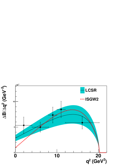
Figure 4: Partial branching fractions (points with error bars) with respect to $q^{2}$. The data are compared with the predictions from light-cone sum rules (LCSR) Ball and Zwicky (2005a) and a quark-model calculation (ISGW2) Scora and Isgur (1995). The uncertainty band (shaded) is given for the LCSR calculation.

Neglecting the theoretical uncertainties, the $\chi^{2}$/NDF of the measured distribution relative to the LCSR prediction Ball and Zwicky (2005a) is 2.4/4, corresponding to a $\chi^{2}$ probability of 67%; relative to the ISGW2 prediction Scora and Isgur (1995) the $\chi^{2}$/NDF is 4.2/4, with a $\chi^{2}$ probability of 40%. Within the large experimental uncertainties, both the LCSR and ISGW2 form factor calculations are consistent with the data. The uncertainties of the ISGW2 form factor calculation are not available. The uncertainties of the LCSR calculation were estimated by the authors to vary linearly as a function of $q^{2}$; i.e., $\sigma_{{\rm d}{\cal B}/{\rm d}q^{2}}/({\rm d}{\cal B}/{\rm d}q^{2})=21\%+3\%\times q^{2}/(14\rm\,Ge\kern-0.80002ptV^{2})$, for the $B\rightarrow\rho\ell\nu$ decays Zwicky (2005). It is assumed that this estimate is also valid for $B^{+}\rightarrow\omega\ell^{+}\nu$ decays.

The value of $|V_{ub}|$ can be determined from the measured partial branching fraction, the $B^{+}$ lifetime $\tau_{+}=(1.638\pm 0.011){\rm\,ps}$ K. Nakamura et al. (2010), and the integral $\Delta\zeta$ of the predicted differential decay rate:

$$|V_{ub}| = \sqrt{\frac{\Delta{\cal B}(q^{2}_{\rm min},q^{2}_{\rm max})}{\tau_{+}\ \Delta\zeta(q^{2}_{\rm min},q^{2}_{\rm max})}}\ ,$$

$$\Delta\zeta(q^{2}_{\rm min},q^{2}_{\rm max}) = {1\over|V_{ub}|^{2}}\int_{q^{2}_{\rm min}}^{q^{2}_{\rm max}}{{\rm d}\Gamma_{\rm theory}\over{\rm d}q^{2}}{\rm d}q^{2}\ .$$ (3)

Table 6 lists the values of $\Delta\zeta$ and $|V_{ub}|$ for LCSR and ISGW2 in different ranges of $q^{2}$. LCSR calculations are more accurate at low $q^{2}$, while ISGW2 predictions are more reliable at high $q^{2}$. Both form factor calculations arrive at very similar values for $|V_{ub}|$. These values of $|V_{ub}|$ are consistent with the more precisely measured values from $B\rightarrow\pi\ell\nu$ decays V. G. Lüth (2011).

Table 6: $|V_{ub}|$, determined from two form factor calculations of $\Delta\zeta$, in different ranges of $q^{2}$. The first uncertainty is experimental (the sum in quadrature of statistical and systematic); the second uncertainty is from theory, and is only available for LCSR.

	$q^{2}$ ($\rm\,Ge\kern-0.80002ptV^{2}$)	$\Delta\zeta({\rm\,ps}^{-1})$	$|V_{ub}|$ ($\times 10^{-3}$)
	0–12	3.9 $\pm$ 0.9	3.37 $\pm$ 0.23 $\pm$ 0.38
LCSR Ball and Zwicky (2005a)	12–21	3.2 $\pm$ 0.8	3.04 $\pm$ 0.32 $\pm$ 0.37
	0–21	7.1 $\pm$ 1.7	3.23 $\pm$ 0.22 $\pm$ 0.38
	0–12	3.6	3.51 $\pm$ 0.24
ISGW2 Scora and Isgur (1995)	12–21	3.4	2.94 $\pm$ 0.31
	0–21	7.0	3.24 $\pm$ 0.22

The value of $\cal B$($B^{+}\rightarrow\omega\ell^{+}\nu$) measured in this analysis supersedes the previous BABAR measurement B. Aubert et al. (2009) based on a smaller data sample, and is in excellent agreement with a recent result J. P. Lees et al. (2012) based on the full BABAR data set. The principal difference between this analysis and the previous ones is that the combinatorial-$\omega$ background is taken from the sideband of the data $m_{3\pi}$ distribution rather than from MC simulation. Although the dominant systematic uncertainties from event reconstruction cannot be avoided, this procedure substantially reduces the reliance on the MC simulation of this largest source of background.

Currently, the QCD predictions of the form factors, and in particular their uncertainties, have limited precision for $B^{+}\rightarrow\omega\ell^{+}\nu$ and $B\rightarrow\rho\ell\nu$ decays. These form factor uncertainties impact $|V_{ub}|$ derived from $\cal B$($B^{+}\rightarrow\omega\ell^{+}\nu$). In the future, form factor calculations with reduced uncertainties combined with improved branching fraction measurements would enable tests and discrimination among different predictions as a function of $q^{2}$, and thereby improve the determination of $|V_{ub}|$.

VII Acknowledgments

We are grateful for the extraordinary contributions of our PEP-II colleagues in achieving the excellent luminosity and machine conditions that have made this work possible. The success of this project also relies critically on the expertise and dedication of the computing organizations that support BABAR. The collaborating institutions wish to thank SLAC for its support and the kind hospitality extended to them. This work is supported by the US Department of Energy and National Science Foundation, the Natural Sciences and Engineering Research Council (Canada), the Commissariat à l’Energie Atomique and Institut National de Physique Nucléaire et de Physique des Particules (France), the Bundesministerium für Bildung und Forschung and Deutsche Forschungsgemeinschaft (Germany), the Istituto Nazionale di Fisica Nucleare (Italy), the Foundation for Fundamental Research on Matter (The Netherlands), the Research Council of Norway, the Ministry of Education and Science of the Russian Federation, Ministerio de Ciencia e Innovación (Spain), and the Science and Technology Facilities Council (United Kingdom). Individuals have received support from the Marie-Curie IEF program (European Union), the A. P. Sloan Foundation (USA) and the Binational Science Foundation (USA-Israel).

References

- (1) The charge conjugate decay mode is implicitly included.
- J. Beringer et al. (2012) J. Beringer et al., Phys. Rev. 86, 010001 (2012), page 1111.
- D. Asner et al. (2010) D. Asner et al. (Heavy Flavor Averaging Group) (2010), eprint e-Print: arXiv:1010.1589 [hep-ex].
- C. Schwanda et al. (2004) C. Schwanda et al. (Belle Collaboration), Phys. Rev. Lett. 93, 131803 (2004).
- I. Adachi et al. (2008) I. Adachi et al. (Belle Collaboration) (2008), eprint 0812.1414.
- B. Aubert et al. (2009) B. Aubert et al. (BABAR Collaboration), Phys. Rev. D79, 052011 (2009).
- Richman and Burchat (1995) J. D. Richman and P. R. Burchat, Rev. Mod. Phys. 67, 893 (1995).
- Ball and Zwicky (2005a) P. Ball and R. Zwicky, Phys. Rev. D71, 014029 (2005a).
- P. del Amo Sanchez et al. (2011) P. del Amo Sanchez et al. (BABAR Collaboration), Phys. Rev. D83, 032007 (2011).
- Scora and Isgur (1995) D. Scora and N. Isgur, Phys. Rev. D 52, 2783 (1995).
- B. Aubert et al. (2002a) B. Aubert et al., Nucl. Instrum. Methods A 479, 1 (2002a).
- Lange (2001) D. J. Lange, Nucl. Instrum. Methods A462, 152 (2001).
- T. Sjöstrand (1994) T. Sjöstrand, Comp. Phys. Commun. 82, 74 (1994).
- S. Agostinelli et al. (2003) S. Agostinelli et al., Nucl. Instrum. Methods A 506, 250 (2003).
- Fazio and Neubert (1999) F. D. Fazio and M. Neubert, J. of High Energy Phys. 6, 17 (1999).
- Becirevic and Kaidalov (2000) D. Becirevic and A. B. Kaidalov, Phys. Lett. B 478 (2000).
- B. Aubert et al. (2007) B. Aubert et al. (BABAR Collaboration), Phys. Rev. Lett. 98, 091801 (2007).
- Ball and Zwicky (2005b) P. Ball and R. Zwicky, Phys. Rev. D 71, 014015 (2005b).
- Isgur and Wise (1989) N. Isgur and M. B. Wise, Phys. Lett. B 232, 113 (1989).
- I. Caprini and Neubert (1998) L. L. I. Caprini and M. Neubert, Nucl. Phys. B530 (1998).
- B. H. Behrens et al. (2000) B. H. Behrens et al. (CLEO Collaboration), Phys. Rev. D 61, 052001 (2000).
- Fox and Wolfram (1979) G. C. Fox and S. Wolfram, Nucl. Phys. B149, 413 (1979).
- B. Aubert et al. (2002b) B. Aubert et al., Phys. Rev. Lett. 89, 011802 (2002b).
- K. Nakamura et al. (2010) K. Nakamura et al. (Particle Data Group), J. Phys. G37, 075021 (2010).
- Barlow and Beeston (1993) R. J. Barlow and C. Beeston, Comput. Phys. Commun. 77, 219 (1993).
- Barberio and Was (1994) E. Barberio and Z. Was, Comput. Phys. Commun. 79, 291 (1994).
- McGregor (2008) G. D. McGregor, Counting at BABAR, MSc Thesis, University of British Columbia, Canada (2008), eprint SLAC-R-912, e-Print: arXiv:0812.1954 [hep-ex].
- Zwicky (2005) R. Zwicky (2005), private communication.
- V. G. Lüth (2011) V. G. Lüth, Ann. Rev. Nucl. Part. Sci. 61, 119 (2011).
- J. P. Lees et al. (2012) J. P. Lees et al. (BABAR Collaboration), Phys. Rev. D86, 092004 (2012).