GPU-accelerated simulation of colloidal suspensions with direct hydrodynamic interactions

Abstract

Solvent-mediated hydrodynamic interactions between colloidal particles can significantly alter their dynamics. We discuss the implementation of Stokesian dynamics in leading approximation for streaming processors as provided by the compute unified device architecture (CUDA) of recent graphics processors (GPUs). Thereby, the simulation of explicit solvent particles is avoided and hydrodynamic interactions can easily be accounted for in already available, highly accelerated molecular dynamics simulations. Special emphasis is put on efficient memory access and numerical stability. The algorithm is applied to the periodic sedimentation of a cluster of four suspended particles. Finally, we investigate the runtime performance of generic memory access patterns of complexity $O\bigl{(}N^{2}\bigr{)}$ for various GPU algorithms relying on either hardware cache or shared memory.

1 Introduction

Micron-sized colloidal particles are suspended in a solvent for most applications. The particle motion couples to the flow field of the solvent, which can significantly affect the dynamic properties. Already the Brownian motion of a single particle in a viscous solvent creates a slowly decaying flow pattern with feedback on the particle at a later point in time. This effect is known as hydrodynamic memory and leads to an experimentally relevant “coloured” noise spectrum Franosch et al. (2011). The flow field due to a steadily dragged particle, first calculated by George G. Stokes, decays slowly with distance and exerts a drag on nearby particles referred to as hydrodynamic interactions. They are intrinsically of many-body nature and in general produce chaotic trajectories with nontrivial and sometimes surprising effects. For example, three colloids driven along a circle exhibit an intriguing cyclic motion Lutz et al. (2006) due to the “peloton effect”: the mobility of a pair of close colloids is enhanced. Another example are sedimenting suspensions in a slit pore, where the formation of complex spatial patterns, related to a Rayleigh–Taylor instability, was observed in experiments and simulations Wysocki et al. (2009); Milinkovic et al. (2011). Further, hydrodynamic interactions enhance the self-diffusion of colloidal particles confined to a fluid interface Rinn et al. (1999) and, in the absence of long-range repulsive forces, accelerate their capillary collapse Bleibel et al. (2011).

Computer simulations of colloidal suspensions including hydrodynamic effects are challenged by the vast amount of solvent molecules per colloid particle. Various techniques have been developed which use coarse-grained solvents to approximate the fluid properties at mesoscopic scales. Popular methods are the lattice-Boltzmann technique and multi-particle collision dynamics, see, e.g., Refs. Dünweg and Ladd, 2009; Gompper et al., 2009; Padding and Louis, 2006 and references therein. In particular for diluted suspensions, such approaches have the drawback that the fluid representation consumes most of the computational resources. Complementary to methods with explicit solvent are Stokesian dynamics simulations Ermak and McCammon (1978); Durlofsky et al. (1987), where the solvent-mediated interactions are accounted for by a many-particle mobility matrix constructed from hydrodynamic tensors leading to deterministic equations of motion. The correct incorporation of Brownian motion Ermak and McCammon (1978) is computationally expensive, and often approximate algorithms are used Banchio and Brady (2003). Here, we restrict to phenomena where Brownian motion is of relatively low importance compared to the overall motion (large Péclet number) and can be neglected, examples can be found in Refs. Bleibel et al., 2011 and Ladd, 1993; Padding and Louis, 2004; Putz et al., 2010.

Computing hardware has seen a paradigm shift during the last decade from single-core processors to highly parallel multi-core architectures. Driven by the consumer market for video games, graphics processing units (GPUs) have been developed that contain several hundred tiny processor cores on a single chip. These subunits are specialised on streaming numerical computations of large data sets in parallel. Today, such streaming processors are often part of new installations in high-performance computing centres.

The success of conventional molecular dynamics simulations on GPUs Baker and Hirst (2011) suggests to exploit the potential of GPUs also for simulation techniques with more complex interactions and advanced algorithms. In general, particle-based continuum simulations are more challenging than lattice models with respect to algorithms and runtime performance Anderson et al. (2008); van Meel et al. (2008) as well as numerical stability and floating-point precision Colberg and Höfling (2011); Ruymgaart et al. (2011). Here, we will specifically address simulations of suspended particles with direct hydrodynamic interactions instantaneously mediated by an implicit solvent. GPUs were used previously to simulate hydrodynamic interactions in suspensions of active dumbbells Putz et al. (2010). A hybrid implementation scheme with explicit solvent is described in Ref. Röhm and Arnold, 2012, where the particles are treated by the host processor(s) and the solvent is modelled as lattice-Boltzmann fluid and propagated by the GPU.

2 Theoretical background

2.1 Stokes equation

The starting point for a mesoscopic description of the solvent is the Navier–Stokes equation for incompressible flow (low Mach number) of Newtonian fluids Batchelor (2000),

$$\varrho\left(\partial_{t}\vec{u}+\vec{u}\cdot\boldsymbol{\nabla}\vec{u}\right)=\eta\nabla^{2}\vec{u}-\boldsymbol{\nabla}p+\vec{f}\,,\qquad\boldsymbol{\nabla}\cdot\vec{u}=0\,,$$ (1)

$\vec{u}=\vec{u}(\vec{r},t)$ denotes the velocity field of the fluid, $\varrho$ the uniform mass density, $\eta$ the shear viscosity, $p=p(\vec{r},t)$ the pressure field, and $\vec{f}=\vec{f}(\vec{r},t)$ an external force density. Such a continuum approach holds at length and time scales much larger than the molecular scales of the solvent (low Knudsen number). The assumption of incompressibility is quite well fulfilled by most fluids at standard temperature and pressure.

Suspended colloidal particles impose additional boundary conditions on the fluid. For not too small particles, there is ample experimental evidence that the fluid molecules at the particle boundary adopt the velocity of the latter, which is referred to as stick boundary conditions,

$$\vec{u}(\vec{r})=\vec{v}+\vec{\Omega}\times(\vec{r}-\vec{r}_{0})\quad\text{for}\quad\vec{r}\in\partial V.$$ (2)

Here, $\vec{v}$ and $\vec{\Omega}$ are the translational and angular velocities of the immersed object, respectively; $\vec{r}_{0}$ is a reference point of the particle and $\partial V$ denotes its surface.

The physics of micron-sized objects like bacteria or colloidal particles is mostly dominated by viscous friction (low Reynolds number), which permits neglecting the inertia term $\varrho\vec{u}\cdot\boldsymbol{\nabla}\vec{u}$ in Eq. (1), known as creeping flow limit. The time scale $\tau$ for the velocity field to adjust to a local disturbance is set by the diffusive propagation of shear waves together with the largest typical length scale $L$ of the problem Dhont (1996); Eckhardt and Buehrle (2008); for water and $L=10$ µm, $\tau\approx\varrho L^{2}/\eta\approx 10^{-4}$ s. For sufficiently slowly changing boundary conditions, the fluid response can be considered instantaneous and the time derivative $\varrho\partial_{t}\vec{u}$ can be dropped as well, which leads to the time-independent Stokes equation,

$$-\eta\nabla^{2}\vec{u}=-\boldsymbol{\nabla}p+\vec{f},\qquad\boldsymbol{\nabla}\cdot\vec{u}=0\,,$$ (3)

which forms the basis of Stokesian dynamics simulations. It has some analogies to the Poisson equation in magnetostatics, from which many concepts can be carried over. The approximation of infinitely fast propagating hydrodynamic interactions is a serious limitation of Stokesian dynamics and needs to be justified for every problem, in particular when considering large system sizes or an externally prescribed time-dependence of the boundaries Eckhardt and Buehrle (2008).

2.2 Hydrodynamic interactions

The flow field $\vec{u}(\vec{r})=\textsf{G}(\vec{r})\cdot\vec{F}$ due to a point force, $\vec{f}(\vec{r})=\vec{F}\,\delta(\vec{r})$, acting on the fluid defines Green’s function of the Stokes equation, the Oseen tensor Oseen (1927),

$$\textsf{G}(\vec{r})=\frac{1}{8\pi\eta r}(\textsf{I}+\vec{\hat{r}}\vec{\hat{r}})\,;$$ (4)

the notation $\vec{a}\vec{b}$ indicates a second-rank tensor with components $(\vec{a}\vec{b})_{\alpha\beta}=a_{\alpha}b_{\beta}$, $\textsf{I}_{\alpha\beta}=\delta_{\alpha\beta}$ is the unit tensor, and $\vec{\hat{r}}=\vec{r}/r$ with $r=|\vec{r}|$. The most prominent property of the Oseen tensor is the slow $1/r$-decay of its magnitude reflecting the long-range nature of hydrodynamic interactions.

The boundary condition, Eq. (2), for the suspended particles can be replaced by an (a priori unknown) induced force density $\vec{f}(\vec{r})$ localised on the particle surfaces, continuing the velocity field inside the particles. By the Stokes equation (3), $\vec{f}(\vec{r})$ generates a flow field $\vec{u}(\vec{r})$, which in general depends on the shapes and orientations of the particles. The contribution $\vec{u}_{0}(\vec{r})$ from a single particle in a quiescent fluid is obtained within a multipole expansion analogously to the treatment in magnetostatics Mazur and van Saarloos (1982). Keeping only the leading, monopole contribution, it reads

$$\vec{u}_{0}(\vec{r})=\int\!\mathrm{d}^{3}r^{\prime}\,\textsf{G}(\vec{r}-\vec{r}^{\prime})\cdot\vec{f}(\vec{r}^{\prime})=\left(1+\frac{a^{2}}{6}\nabla^{2}\right)\textsf{G}(\vec{r})\cdot\vec{F}+O\bigl{(}r^{-4}\bigr{)}\quad\text{for}\quad r\gg a,$$ (5)

with total force $\vec{F}=\int\!\vec{f}(\vec{r})\,\mathrm{d}^{3}r$, (root-mean-square) radius of the particle surface $a$, and the particle being centred at the coordinate origin. An external drag force can be included in the force monopole, and the flow field for many particles is found by superposition of the single particle contributions.

The velocity distribution on the surface of another particle at position $\vec{r}$ may be expanded in multipoles as well, the monopole term yields just the particle’s translational velocity $\vec{v}$; its computation is facilitated by Faxén’s theorem Dhont (1996),

$$\vec{v}=\frac{1}{4\pi a^{2}}\int_{\partial V(\vec{r})}\!\vec{u}(\vec{r}^{\prime})\,\mathrm{d}^{3}r^{\prime}=\left(1+\frac{a^{2}}{6}\nabla^{2}\right)\vec{u}(\vec{r}).$$ (6)

The velocity dipole determines the angular velocity, and higher terms vanish for stick boundary conditions. Rotational motion leads to a coupling between velocity and force monopoles, which is of order $r^{-4}$ and, at the monopole level, limits the consistent expansion of Eq. (5) to the third order in distance.

Combining Eqs. (5) and (6) for $N$ particles encodes the hydrodynamic interactions in a configuration-dependent many-body mobility matrix $\textsf{\textmu}_{ij}(\vec{r}_{1},\dots,\vec{r}_{N})$ relating forces to velocities,

$$\vec{v}_{i}=\sum_{j=1}^{N}\textsf{\textmu}_{ij}\cdot\vec{F}_{j}=\mu_{0}\vec{F}_{i}+\sum_{j\neq i}^{N}\textsf{T}(\vec{r}_{i}-\vec{r}_{j})\cdot\vec{F}_{j}\quad\text{for}\quad i=1,\dots,N;$$ (7a)

Latin subscripts refer to particle indices. The self-contribution $${\textsf{\textmu}}_{ii} \mu_{0}=1/6\pi\eta a$$ describes the direct effect of a drag force on the particle itself and is set by the Stokes mobility, . The off-diagonal terms are given by the Rotne–Prager tensor,

$$\textsf{T}(\vec{r})=\left(1+\frac{a^{2}}{3}\nabla^{2}\right)\textsf{G}(\vec{r})=\mu_{0}\frac{3a}{4r}(\textsf{I}+\vec{\hat{r}}\vec{\hat{r}})+\mu_{0}\frac{a^{3}}{2r^{3}}(\textsf{I}-3\vec{\hat{r}}\vec{\hat{r}})\,.$$ (7b)

If the particle size is negligible compared to the particle separation, the gradients in Eqs. (5) and (6) may be dropped, replacing T by the Oseen tensor G. An advantage of the Rotne–Prager tensor, necessary for the simulation of Brownian motion, is that the matrix µ is positive definite if no pair of particle centres is closer than $2a$ Rotne and Prager (1969).

2.3 Lubrication correction

If two particles come close together, the hydrodynamic coupling is only poorly described by the far-field expansion. In particular, the many-body friction matrix, $\boldsymbol{\zeta}=\textsf{\textmu}^{-1}$, becomes singular if only a thin lubrication film separates the particle surfaces. Cox (1974) computed the leading singularities for two approaching surfaces of arbitrary shape, and asymptotic expansions for two spheres were given by Jeffrey and Onishi (1984). Let us introduce relative positions and velocities, $\vec{r}_{ij}=\vec{r}_{i}-\vec{r}_{j}$ and $\vec{v}_{ij}=\vec{v}_{i}-\vec{v}_{j}$, and the dimensionless separation between particle surfaces, $s_{ij}=r_{ij}/a-2$. Then, the singular part of the force on sphere $i$ due to a sphere $j$ moving nearby reads Jeffrey and Onishi (1984)

$$\mu_{0}\vec{F}^{\text{sing}}_{i}=\left[\frac{1}{4s_{ij}}-\frac{9}{40}\log(s_{ij})\right]\vec{\hat{r}}_{ij}\vec{\hat{r}}_{ij}\cdot\vec{v}_{ij}-\frac{1}{6}\log(s_{ij})\,(\textsf{I}-\vec{\hat{r}}_{ij}\vec{\hat{r}}_{ij})\cdot\vec{v}_{ij}+O\bigl{(}s_{ij}^{0}\bigr{)}\,,$$ (8)

again ignoring contributions from rotational motion. We truncate ad hoc at $s_{ij}=1$ or $r_{ij}=3a$, where the logarithm changes its sign, avoiding a sign change of the lubrication forces in the present approximation. The lubrication correction to the many-body friction matrix is constructed from close particle pairs alone, such that $\vec{F}^{\text{sing}}_{i}=\sum_{j}\boldsymbol{\zeta}^{\text{sing}}_{ij}\vec{v}_{j}$. The result from lubrication theory has to be matched with the far-field expansion of the inverse mobility matrix Durlofsky et al. (1987); Ladd (1990). Since we kept only the singular terms of $\boldsymbol{\zeta}$ in Eq. (8) it can simply be added,

$$\textsf{v}=\left(\textsf{\textmu}^{-1}+\boldsymbol{\zeta}^{\text{sing}}\right)^{-1}\textsf{F}=\textsf{\textmu}\left(\textsf{I}+\boldsymbol{\zeta}^{\text{sing}}\textsf{\textmu}\right)^{-1}\textsf{F}\,.$$ (9)

3 Simulation algorithm and implementation

3.1 Algorithm

The idea behind Stokesian dynamics simulations is to avoid the explicit simulation of the individual solvent molecules as one would do in traditional molecular dynamics simulations. Rather, hydrodynamic interactions between colloidal particles are properly incorporated by means of the many-body mobility matrix µ defined in Eq. (7). This matrix is entirely constructed from pair contributions, even at higher orders of the multipole expansion.

Our main motivation for including the lubrication correction is the implementation of a hard core repulsion. Hence, we suggest the approximation $\textsf{v}\approx\textsf{\textmu}\bigl{(}\textsf{I}-\boldsymbol{\zeta}^{\text{sing}}\textsf{\textmu}\bigr{)}\textsf{F}$ to Eq. (9), which avoids the storage and inversion of the $3N\times 3N$ matrix µ. Further, we approximate on the right-hand side $\textsf{\textmu}\boldsymbol{\zeta}^{\text{sing}}\textsf{\textmu}\textsf{F}\approx\textsf{\textmu}\boldsymbol{\zeta}^{\text{sing}}\textsf{v}$ using the velocities from the previous simulation step; effectively, the particle forces are corrected for lubrication before the velocity update. Then, the simulation algorithm consists of repeating the following steps:

1. update particle positions:
   $\vec{r}_{i}\leftarrow\vec{r}_{i}+\delta t\,\vec{v}_{i}$

2. compute forces on each particle due to external forces, interactions, and lubrication:
   $\textsf{F}_{i}\leftarrow\vec{F}_{i}^{\text{ext}}(\vec{r}_{i})+\sum_{j}^{\prime}\vec{F}_{i}^{\text{int}}(\vec{r}_{i},\vec{r}_{j})-\sum_{j}^{\prime}\boldsymbol{\zeta}^{\text{sing}}_{ij}(\vec{r}_{i},\vec{r}_{j})\cdot(\vec{v}_{i}-\vec{v}_{j})$

3. compute particle velocities via mobility matrix:
   $\vec{v}_{i}\leftarrow\sum_{j}\textsf{\textmu}_{ij}(\vec{r}_{i},\vec{r}_{j})\cdot\vec{F}_{j}$

Particle positions are propagated by a simple Euler integration in step 1. The primed sums in step 2 can be accelerated by Verlet neighbour lists common for short-ranged forces as described, e.g., in Ref. Colberg and Höfling, 2011. Since the hydrodynamic interactions are long-ranged, like electrostatics or gravity, it is preferable to keep all interactions of every pair of particles and not to cut off at some short distance. Thus, the sum in step 3 is the computationally most intense part involving $N^{2}$ contributions for all $N$ particles; the mobility matrix itself, however, need not be stored in memory.

3.2 GPU implementation

The present work relies on the “compute unified device architecture” (CUDA) introduced by the Nvidia Corporation CUD (2010). It provides some abstraction to the actual GPU hardware and makes Nvidia GPUs freely programmable using the C++ language. The central concept is thread parallelism, which means that several hundred or thousand program threads execute the same routine on the GPU, the latter is referred to as “kernel”. Each group of (currently) $M=32$ threads forms a “warp”, several warps are organised into a thread block, and all blocks together represent the full set of threads. The threads within a warp execute simultaneously, but the execution order of warps is not guaranteed. The warps comprising a block are resident on the same multiprocessor and execute independently, the size of a block is limited by the available hardware resources. Communication between threads is only supported within the same block using “shared” memory, which does not persist beyond the lifetime of the block. Data input and output of a kernel occurs through the “global” memory, which is the only persistent type of memory on the GPU board. Despite the high overall bandwidth of global memory, each memory transaction entails a huge latency of several hundred clock cycles, which is, however, partly hidden by the thread scheduler on the chip. Optimal access to global memory is ensured if a warp of threads reads from or writes to a sequence of contiguous memory locations that fit within a single, properly aligned window of 64 or 128 bytes. Then, the memory access of the whole warp is coalesced into a single transaction of a large block. As another remedy for the high memory latency, the Nvidia GPUs of CUDA compute capability $\geq 2.0$ (“Fermi”) have been equipped with hardware caches. We put particular attention to memory transfer because it is typically the bottleneck of a GPU program; it appears to become the limiting factor in conventional high-performance computing as well. We are not concerned with memory transfer between host system and GPU device since our simulation algorithms are fully implemented for the GPU.

Algorithm 1 Pseudo code of the CUDA kernel for updating the particle velocities in the naïve implementation, for an illustration see Fig. 1a. The kernel is executed concurrently by at least $N$ threads, array indices are 1-based, and arrays in global memory are denoted by capital letters.

1:function update_velocity(position array $\vec{R}$, velocity array $\vec{V}$, force array $\vec{F}$, #particles $N$, …)

2:     local $j\leftarrow\text{global thread ID}$

3:     local $\vec{r}\leftarrow\vec{R}_{j}$ $\triangleright$ read from global memory

4:     local $\vec{v}\leftarrow 0$

5:     for $k$ from 1 to $N$ do $\triangleright$ loop over all particles

6:         local $\vec{r}^{\prime},\vec{f}^{\prime}\leftarrow\vec{R}_{k},\vec{F}_{k}$ $\triangleright$ read from global memory

7:         if $j=k$ then $\triangleright$ velocity contribution according to Eq. (7)

8:              $\vec{v}\leftarrow\vec{v}+\mu_{0}\,\vec{f}^{\prime}$. $\triangleright$ self-contribution

9:         else

10:              $\vec{v}\leftarrow\vec{v}+\textsf{T}(\vec{r}-\vec{r}^{\prime})\cdot\vec{f}^{\prime}$. $\triangleright$ use hydrodynamic tensor

11:         end if

12:     end for

13:     $\vec{V}_{j}\leftarrow\vec{v}$ $\triangleright$ write to global memory

14:end function

a	b
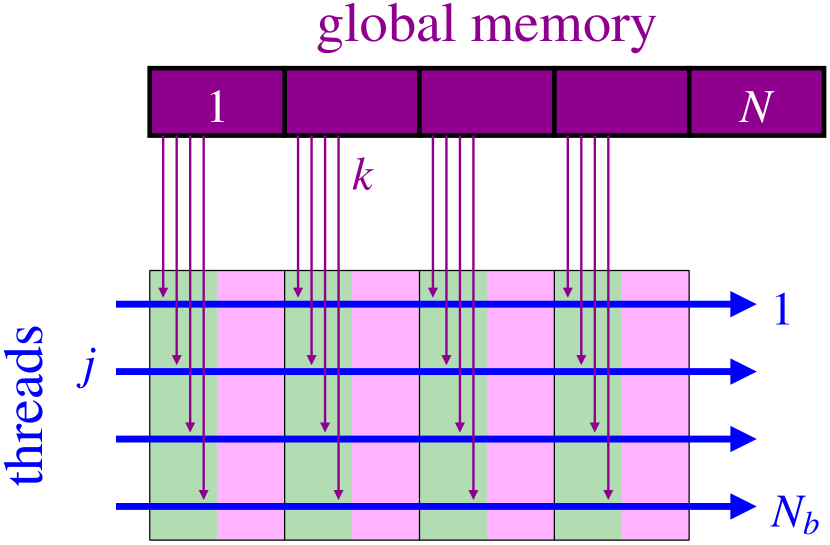
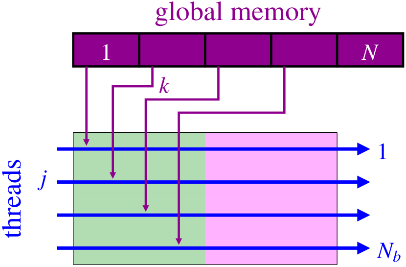
c	d

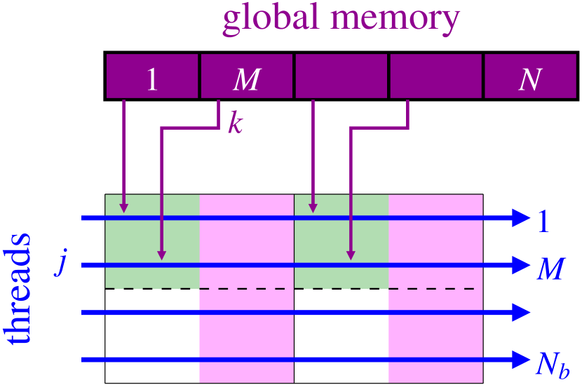
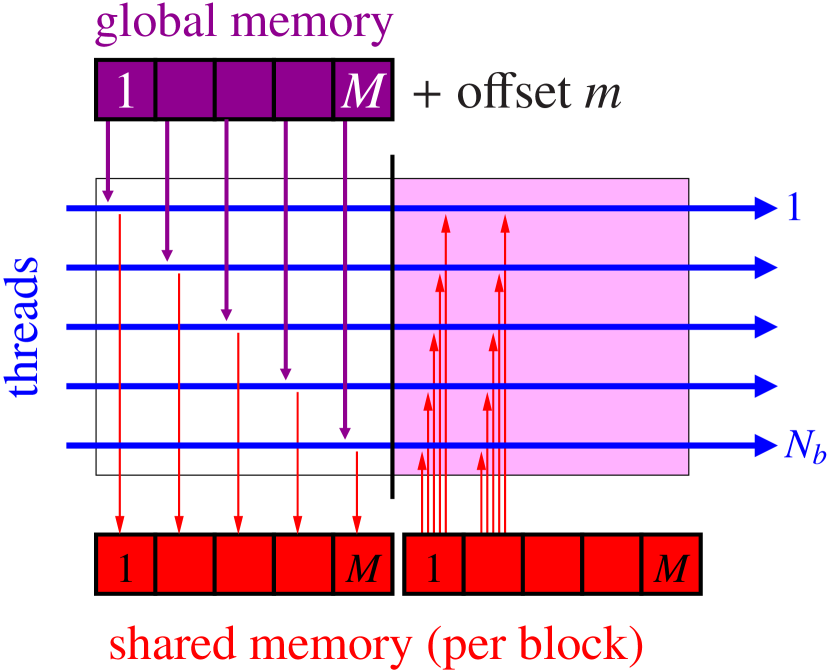
Figure 1: Visualisation of various algorithms for the computation of hydrodynamic interactions, see Algorithms 1 and 2. Blue horizontal arrows represent the threads being associated with one particle each, gradually computing hydrodynamic interactions with all $N$ particles (purple boxes on top); only one block of $N_{b}$ threads is shown. Purple, vertical arrows represent global memory accesses; green rectangles symbolise data fetching and pink ones data processing, i.e., the actual computation.  (a) naïve implementation. Data of one particle at a time are read from global memory directly without caching.  (b) tiling algorithm. Data are read from global memory by coalesced transactions and are stored blockwise in shared memory for further processing.  (c) small-tiling algorithm using small tiles of size $M$, it is similar to the tiling algorithm, but the coalesced read is performed only by one warp of each thread block (delimited by the dashed line).  (d) access to shared memory (red arrows/box) within one thread block for the tiling ($M=N_{b}$) and small-tiling algorithms.

The most straightforward implementation of step 3 on a GPU is to assign one thread to each particle, which computes and accumulates the contributions from all $N$ particles (including the self-contribution) to the velocity of the thread’s particle, see Algorithm 1. The symmetry $\textsf{\textmu}_{jk}=\textsf{\textmu}_{jk}^{T}$ will not be made use of for the same reason why Newton’s third law is not exploited for the computation of forces from pair interactions: transferring the result from thread $j$ to an arbitrary thread $k$ would break thread parallelism and would require a sophisticated communication pattern involving a bloat of global memory transactions. The kernel basically consists of a loop over all particles, sequentially reading and processing their positions and forces from global memory. Before exit, the kernel stores the computed velocity, which is the only global write operation. The threads within a warp can diverge (line 7) due to the self-contribution of a particle to its velocity, which unavoidably happens once for every thread in a warp and does not seem to significantly impact the execution time.

Algorithm 2 The small-tiling variant of algorithm 1. Position and force data are partitioned in small tiles and prefetched into shared memory by the first warp of each block, for an illustration see Fig. 1c,d. Arrays in shared memory are denoted by a tilde.

1:function update_velocity(position array $\vec{R}$, velocity array $\vec{V}$, force array $\vec{F}$, #particles $N$, …)

2:     local $j\leftarrow\text{global thread ID}$

3:     local $n\leftarrow\text{thread ID within block}$

4:     local $M\leftarrow\text{warp size}$

5:     allocate shared memory $\tilde{\vec{r}}[M],\tilde{\vec{f}}[M]$ $\triangleright$ positions, forces

6:     local $\vec{r}\leftarrow\vec{R}_{j}$ $\triangleright$ read from global memory

7:     local $\vec{v}\leftarrow 0$

8:     for $m$ from $1$ to $N$ with stride $M$ do $\triangleright$ loop over all particles in tiles of size $M$

9:         if thread in first warp then

10:              $\tilde{\vec{r}}_{n},\tilde{\vec{f}}_{n}\leftarrow\vec{R}_{m+n},\vec{F}_{m+n}$ $\triangleright$ copy from global to shared memory

11:         end if

12:         synchronise threads $\triangleright$ wait until data are fetched

13:

14:         for $k$ from $1$ to $M$ do $\triangleright$ loop over fetched data

15:              local $\vec{r}^{\prime},\vec{f}^{\prime}\leftarrow\tilde{\vec{r}}_{k},\tilde{\vec{f}}_{k}$ $\triangleright$ read from shared memory

16:              if $j=m+k$ then $\triangleright$ velocity contribution according to Eq. (7)

17:                  $\vec{v}\leftarrow\vec{v}+\mu_{0}\,\vec{f}^{\prime}$. $\triangleright$ self-contribution

18:              else

19:                  $\vec{v}\leftarrow\vec{v}+\textsf{G}(\vec{r}-\vec{r}^{\prime})\cdot\vec{f}^{\prime}$. $\triangleright$ use hydrodynamic tensor

20:              end if

21:         end for

22:         synchronise threads $\triangleright$ wait until data are processed

23:     end for

24:     $\vec{V}_{j}\leftarrow\vec{v}$ $\triangleright$ write to global memory

25:end function

Following Nyland et al. (2007), the naïve read pattern in line 6 is excessively inefficient: first, the same location in memory is accessed by every thread (Fig. 1a) and, second, memory bandwidth is wasted. The requirements for optimal memory access can be met by tiling the matrix of $N\times N$ interactions into squares of size $N_{b}$ Nyland et al. (2007), see Fig. 1b; a similar approach has been proposed for general matrix multiplication CUD (2010). $N_{b}$ denotes the number of threads per block, it varies typically between 128 and 1024. The interactions are processed tile by tile and the data for a tile are cached in shared memory, making them available to all threads within the block (Fig. 1d), and reducing the number of global memory reads by a factor of $N_{b}/M$. For gravity Nyland et al. (2007) or matrix multiplication CUD (2010), the size of a data item is smaller than in our case of hydrodynamic interactions. Here, the information per particle comprise two three-dimensional vectors, a position and a force, amounting to 32 bytes per particle (2 × float4) if alignment restrictions are obeyed. The relatively high shared memory usage of $32\times M=1024$ bytes per warp limits the multiprocessor occupancy on older hardware (CUDA compute capability < 2.0) with a potential increase of kernel execution time; for compute capability 2.0, maximum occupancy is exhausted by 1 kb of shared memory per warp CUD (2010). The shared memory usage can be significantly reduced without increasing the volume of global memory transfer if merely the first warp of a block fetches the data, the tiles become of rectangular shape $M\times N_{b}$. The resulting small-tiling version is displayed in Algorithm 2 and illustrated in Fig. 1c. The original tiling algorithm is recovered by replacing $M$ with the block size and removing the condition in line 9.

Data fetching from global memory uses adjacent memory locations and allows for coalescable access (line 10), in contrast to line 6 of Algorithm 1. It is followed by a synchronisation barrier (line 12) to prevent the other warps from premature reading from shared memory. The condition in line 9 does not break convergent thread execution within each warp (the condition is fulfilled either by each thread of a warp or by none), and only memory access within a warp is eligible for coalesced transactions. We see only the slight disadvantage with respect to execution time that fewer transactions are pending on a multiprocessor, which impedes latency hiding by the scheduler. After data fetching is completed, all threads of the block read from shared memory and compute the velocity contribution from hydrodynamic interactions for their respective particle. The tile is closed by another synchronisation barrier (line 22) signalling that the cached data may be overwritten.

The velocity sum in Eq. (7) contains contributions of very different magnitude since the terms decay like the inverse particle separation, $1/r_{ij}$. Conveying the experience from conventional MD simulations Colberg and Höfling (2011), the numerical error can significantly be reduced if the accumulation in line 19 of Algorithm 2 is performed with higher floating-point precision, whereas the hydrodynamic tensor and the forces are computed in single, 24-bit precision. Still reading particle positions and forces in single precision keeps down the memory transfer volume. For CUDA compute capability $\geq 2.0$, native double precision may be used, for older hardware, an emulation via double-single arithmetic is available and can even be more efficient Colberg and Höfling (2011). Finally, since an all-pairs interaction does not involve selective reading, e.g., via Verlet neighbour lists, the physical positions of the particles do not affect the kernel execution time and particle reordering is not necessary. It is, however, required for the efficient computation of interparticle forces and the lubrication correction.

3.3 Runtime performance

a	b

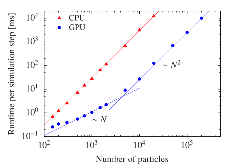
Figure 2: (a) Simulation runtime per step for the computation of hydrodynamic interactions using CPU and GPU implementations of Algorithm 2; straight lines are fits to the regimes of linear and quadratic scaling with particle number.  (b) Relative contributions to the total GPU runtime from the computation of hydrodynamic interactions (hatched bars memory access only, without computation), of lubrication forces, and integration of the equations of motion; the chosen particle numbers correspond to the two scaling regimes and the crossover region.

The described scheme for the computation of hydrodynamic interactions, Algorithm 2, has been implemented as a module extending HAL’s MD package Colberg and Höfling (2008–2012), which forms the basis for the following measurements of runtime performance. The benchmarks mimic the simulation of a sedimenting suspension: all particles experience the same constant drag force $\vec{F}=(0,0,-F)$ due to their buoyant weight, which together with the particle radius $a$ and the Stokes mobility $\mu_{0}$ defines the unit of time, $\tau_{s}=a/\mu_{0}F$. The particles were initially placed on an fcc lattice with a fixed number density of $n=N/L^{3}=0.1a^{-3}$, and the number of particles $N$ was varied between 150 and 200,000. Particle positions were propagated by the Euler integrator using a timestep of $0.001\tau_{s}$, and simulations were run for 100 steps. The GPU hardware for the benchmarks was an Nvidia Tesla C2050, the program was compiled with the CUDA software development kit (SDK) version 4.0 using the option –arch sm_13, and kernels were launched with 512 threads per block. Note that the simulations were about 2.3-times slower on the same hardware if the compiler optimised for the actual target architecture with –arch sm_20, probably due to a different implementation of floating-point arithmetic. For reference, we compare with an equivalent serial implementation for the CPU (Intel Xeon E5620 clocked at 2.40 GHz), with the only difference that the symmetry $\textsf{\textmu}_{ij}=\textsf{\textmu}_{ji}$ is exploited.

The measured runtimes per simulation step are displayed in Fig. 2. One infers clearly that the runtime of the GPU implementation scales quadratically in $N$ for large system sizes, while it grows only linearly for $N\lesssim 2,000$ particles. The former quadratic scaling is also found for the CPU version for all particle numbers, simply reflecting that the interaction between all particle pairs requires $O\bigl{(}N^{2}\bigr{)}$ computations. In the scaling regime, the speedup factor of the GPU over the CPU is about 120. The linear scaling for not too large particle numbers originates from a partial usage of GPU resources: doubling the number of particles, the execution time of each CUDA thread doubles, but so does the number of threads running concurrently. In summary, the total kernel runtime only doubles. When the device capacity is exhausted not all threads can run in parallel anymore, yielding the quadratic increase of the runtime with the number of particles. A small performance gain of 13% is achieved by computing the hydrodynamic interactions only to order $O\bigl{(}r^{-1}\bigr{)}$, i.e., in the Oseen approximation.

In Section 3.2, we developed the small-tiling algorithm for efficient access to global memory. Surprisingly, we found that a variant of the eventual kernel for the computation of hydrodynamic interactions using the naïve memory access pattern slightly outperforms the more sophisticated algorithm, the runtime in the scaling regime is reduced by 8%. This observation motivated us to scrutinise the performance of the different memory access algorithms depending on the specific access pattern, see Appendix A. For linear data access, the naïve implementation performs increasingly better as the size of the individual data elements increases, and finally the overhead of data caching penalises the tiling algorithms. In the present case, both criteria are met: particle data are laid out linearly and 32 bytes are read for each interaction.

4 Numerical stability: periodic sedimentation of four spheres

a	b

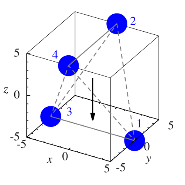
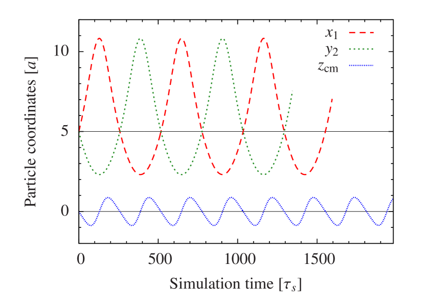
Figure 3: Periodic sedimentation of four equal spheres.  (a) Initial configuration of the particles on the edges of a stretched tetrahedron, edges of equal length are symbolised by equal line patterns. Gravity acts downwards as indicated by the arrow.  (b) Periodic trajectories for two selected coordinates of particles 1 and 2 and the vertical component of the centre of mass, $z_{\text{cm}}$, after correcting for the average sedimentation motion.

In Stokesian dynamics simulations, there are no obvious conserved quantities like energy or momentum, but one may exploit a symmetry to examine the numerical stability of the simulation. The Stokes equation (3) is invariant under time reversal ($\vec{u}\mapsto-\vec{u}$) if positions and forces are reversed as well, $\vec{r}\mapsto-\vec{r}$, $\vec{f}\mapsto-\vec{f}$. The symmetry of the Stokes flow is preserved for fore-and-aft-symmetric particle configurations, i.e., for boundaries invariant under $\vec{r}\mapsto-\vec{r}$. These observations can be used to construct a cyclic motion in an external gravitational field Tory et al. (1991): four equal particles are initially positioned at the vertices of a stretched tetrahedron with two opposing edges perpendicular to the force, see Fig. 3a. After a quarter period, all particles will be in a horizontal plane, and after sedimenting for another quarter period, the horizontally mirrored initial configuration is recovered. After another half period, the initial (relative) configuration is exactly restored. For the initial positions, we placed two horizontally aligned and vertically separated couples of particles at $\vec{r}_{1}=(0,0,5a)$, $\vec{r}_{2}=(0,5a,0)$, $\vec{r}_{3}=-\vec{r}_{1}$, $\vec{r}_{4}=-\vec{r}_{2}$; each particle is dragged downwards by a force $\vec{F}=(0,0,-F)$. The trajectories are determined by a set of merely three different coordinates, e.g., $x_{1}(t)$, $z_{1}(t)$ and $z_{2}(t)$, see Fig. 3b, the remaining components follow by symmetry: $x_{3}(t)=-x_{1}(t)$, $y_{2}(t)=-y_{4}(t)$ being equal to $x_{1}(t)$ shifted in phase by half a period, $z_{3}(t)=z_{1}(t)$, $z_{4}(t)=z_{2}(t)$, and $y_{1}=y_{3}=x_{2}=x_{4}\equiv 0$. The centre-of-mass position, $z_{cm}(t)=[z_{1}(t)+z_{2}(t)]/2$, decreases monotonically, but oscillates around the average sedimentation motion.

The cycle duration is about $T=517\tau_{s}$ long, we have performed long simulations over almost 1000 cycles (50 million steps with an integration timestep of $0.01\tau_{s}$) in order to monitor the numerical stability. The maxima and minima of $x_{1}(t)$ were determined by parabolic fits yielding the cycle duration and the amplitude of the motion, the cycle duration was averaged over time windows of $10^{4}\tau_{s}$. We compare implementations which use either single or double-single floating-point precision Colberg and Höfling (2011) for the accumulation of (a) velocities due to hydrodynamic interactions, Eq. (7), and (b) positions in the Euler integration of the equations of motion. The contributions to the hydrodynamic interactions from different particles vary strongly for close and distant particles due to the $1/r$ prefactor; hence, large and small numbers of different sign are summed with great potential for numerical issues due to limited floating-point precision.

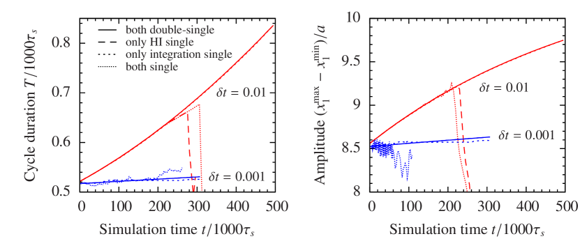
Figure 4: Cycle duration and amplitude of the periodic motion over the course of a very long simulation run using different floating-point precision for the accumulation of hydrodynamic interactions (HI) and positions (integration of the equations of motion); the two datasets refer to different integration timesteps, $\delta t=0.001\tau_{s}$ and $\delta t=0.01\tau_{s}$ as indicated. Note that some curves collapse with the case “both double-single precisison”.

Over the course of the simulation, both the cycle duration and the amplitude display a drift independently of the floating-point precision, see Fig. 4. The motion, however, remains cyclic if double-single precision is used for the accumulation of hydrodynamic interactions. Otherwise, the periodic motion falls apart after some 400 cycles for the larger timestep, regardless of the precision used for the integration. Using the smaller timestep $\delta t=0.001\tau_{s}$ for the integration of positions, the drift is significantly reduced and the cyclic motion remains stable over the full simulation run of more than 500 cycles. The small timestep in conjunction with single precision for both the accumulation of hydrodynamic interactions and the integration leads to a wildly fluctuating cycle duration and amplitude, probably because the low floating-point precision fails to properly resolve the small increments. Note that a smaller drift and an improved stability may be achieved by resorting to higher-order or implicit integration schemes rather than decreasing the timestep; a semi-implicit scheme has been suggested if lubrication forces are included Nguyen and Ladd (2002). The stability issues, however, are likely to persist if merely single floating-point precision is used throughout.

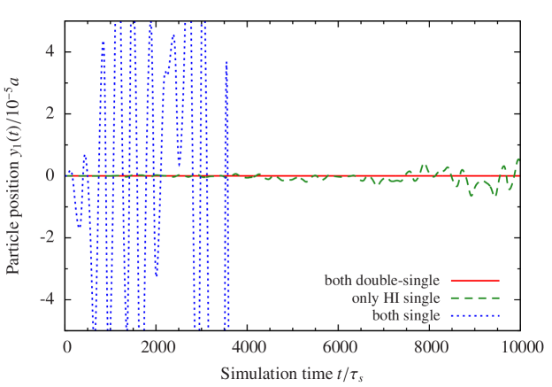
Figure 5: Deviation of particle 1 from the $xz$-plane quantifying the numerical error. Accumulation with different floating-point precision is compared like in Fig. 4.

Another sensitive criterion for numerical stability is that particles initially positioned in the $xz$-plane (particles 1 and 3) should for symmetry reasons remain in this plane during the simulation. Thus, a non-zero $y$-coordinate quantifies the numerical error, the results are shown in Fig. 5 using $\delta t=0.001\tau_{s}$. Note the much shorter simulation runs compared to Fig. 4, the criterion here is much more sensitive to detect numerical inaccuracies. If double-single precision is used for the accumulation of hydrodynamic interactions, we find $y_{2}(t)\equiv 0$, independently of the precision of the integration. Slowly growing deviations are observed if only the hydrodynamic interactions are accumulated in single precision, and large errors arise quickly for positions integrated in single precision as well.

In conclusion, the floating-point precision in the accumulation of hydrodynamic interactions impacts the long-time stability of the described simulation for only four particles, and it is likely to become more relevant for larger setups with a large distribution of particle separations. For the tests discussed, the precision of position integration is less crucial as long as the hydrodynamic interactions are accumulated with increased floating-point precision, but we consider it good practice to do so for the integration as well.

5 Conclusion

We have described a GPU accelerated implementation of Stokesian dynamics simulations, a scheme for dynamic simulations of a particulate suspension that includes direct, instantaneous hydrodynamic interactions and avoids the explicit simulation of the solvent. Our treatment is restricted to the leading order of a multipole expansion, thus neglecting rotational motion, but can in principle be extended to higher orders. The implementation is available in HAL’s MD package Colberg and Höfling (2008–2012) from version 0.2, an efficient simulation software specifically designed to run entirely on the GPU, thereby avoiding the costly data transfer between host and GPU memory; it further supports selected computations with increased floating-point precision for an optimal balance between numerical stability and runtime performance. Since access to global memory on the GPU often limits the execution speed of compute kernels, we have put particular emphasis on the memory access patterns. Explicit data caching by means of the shared memory was compared to the hardware cache available in the latest generation of Nvidia GPUs. Dedicated algorithms using shared memory are in general more efficient for non-linear memory access. For linear access, they show advantages for small data sizes, the straightforward direct memory access, however, turned out to be an equally fast (or even slightly faster) alternative for the computation of hydrodynamic interactions, where a relatively large amount of data (32 bytes) has to be transferred for each particle.

The computation of the long-range hydrodynamic interactions requires to consider all pairs of particles in the simulation box, yielding an algorithmic complexity of order $O\bigl{(}N^{2}\bigr{)}$ for $N$ particles. This scaling is reflected in the runtime for large systems, and we observed a speedup of about 120 compared to the serial reference implementation for a conventional CPU. For up to 2,000 particles however, the runtime scales linearly on the employed GPU hardware since only a fraction of the available computing resources is used.

Other simulation approaches for particulate suspensions treat the solvent explicitly, which typically results in a linear algorithmic complexity. For fixed particle number, the prefactor is proportional to the solvent volume, or equally, the inverse of the colloid volume fraction. Röhm and Arnold (2012) describe molecular dynamics simulations of particles suspended in a GPU-accelerated lattice-Boltzmann solvent. For comparison, they report that one integration step takes about 0.9 ms for 4,150 particles in a solvent of $24^{3}$ lattice nodes, which is to be contrasted with 5.7 ms obtained in this work. Note that the execution time for Stokesian dynamics is merely a function of the absolute particle number, while for the lattice-Boltzmann method it crucially depends on the particle density and the resolution of the solvent lattice. Hence, Stokesian dynamics will in general perform better for dilute suspensions. Similarly, Pham et al. (2009) compared both methods (including Brownian motion) for a polymer chain in solution using conventional hardware and found Stokesian dynamics to be an order of magnitude faster even for chain lengths of 1000 monomers, despite the asymptotically favourable scaling of the lattice-Boltzmann method. Apart from aspects of computational performance, a comparison of methods with implicit and explicit solvent may be interesting from a theoretical point of view for specific problems in physics. It would permit assessing the physical quality of the various approximations introduced by both methods.

The hydrodynamic interactions are related in nature to other long-range interactions, e.g., gravity or electrostatic interactions, and it seems natural to convey more elaborate algorithms from there to the hydrodynamic case, an example being Ewald summation techniques Sierou and Brady (2001). Another interesting approach are fast-multipole methods and tree codes with $O(N\log(N))$ scaling, where remote particle groups are replaced by their multipole moments; Bédorf et al. Bédorf et al. (2012); Bédorf and Zwart (2012) describe an implementation of a Barnes–Hut tree code for gravity fully executing on the GPU, which is able to process 2.8 million particles per second.

Finally, one would like to amend the simulations by Brownian motion Ermak and McCammon (1978); Banchio and Brady (2003), which involves an additional noise term. In order to satisfy the detailed balance condition, a correct computation of the noise strength requires a Cholesky decomposition of the many-body mobility matrix µ, which is computationally expensive and entails a substantial memory footprint. Nevertheless, such a task seems to be well suited for a future GPU implementation.

Appendix A   Data caching for memory access patterns of complexity $O\bigl{(}N^{2}\bigr{)}$

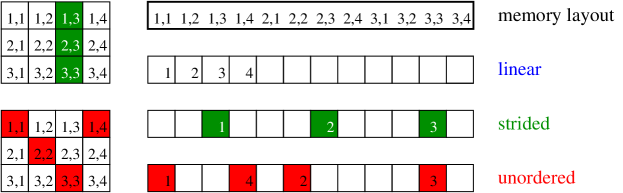
Figure 6: Illustration of the different access patterns. Data are assumed to represent a $3\times 4$ matrix (left) stored in row-major order (white bar on top). “Linear” data access corresponds to reading a row of the matrix, “strided” access reads a column, and “unordered” access reads along a diagonal depending on the offset. Single numbers denote the sequence of data access, and comma-separated pairs indices of matrix elements.

In this appendix, we study the efficiency of data caching using shared memory or hardware caches for different memory access patterns of complexity $O\bigl{(}N^{2}\bigr{)}$, which occur in the computation of all-pairs interactions or in basic linear algebra problems (BLAS). The study was motivated by the somewhat unexpected observation that the two implementations of global memory access in Algorithms 1 and 2 yielded similar execution times, even on older GPU hardware without memory cache. Three different memory access patterns, depicted in Fig. 6, are addressed: linear, linear with a fixed stride, and unordered scattered.

Algorithm 3 Minimalist naïve kernel for benchmarking memory access.

template <typename T>
__global__ void naive(T* g_out, T const* g_in, unsigned N)
{
    unsigned const j = GTID;                     // global thread ID
    T sum = g_in[j];                             // read from global memory
    for (unsigned k = 0; k < N; ++k)
        sum += g_in[map(k)];                     // read from global memory
                                                 // and a trivial computation
    g_out[j] = sum;                              // write to global memory
} 

Algorithm 4 Minimalist small-tiling kernel. The “tiling” algorithm is obtained by substituting warpSize with the size of the execution blocks; the condition n < warpSize in line 10 then always evaluates to true and can be dropped.

template <typename T>
__global__ void smalltiling(T* g_out, T const* g_in, unsigned N)
{
    unsigned const j = GTID;                     // global thread ID
    unsigned const n = TID;                      // thread ID within block
    extern __shared__ T s_data[];                // declare shared memory
    T sum = g_in[j];                             // read from global memory

    for (unsigned m = 0; m < N; m += warpSize) {
        if (n < warpSize)
            s_data[n] = g_in[map(m+n)];          // copy from global to
        __syncthreads();                         // shared memory

        for (unsigned k = 0; k < warpSize; ++k)
            sum += s_data[k];                    // a trivial computation
        __syncthreads();
    }
    g_out[j] = sum;                              // write to global memory
} 

We reduced the algorithms of Section 3 as much as possible to concentrate on memory access. A minimal computation though was included in order to prevent the compiler from optimising out superfluous read statements. The three minimalist CUDA kernels are given in Algorithms 3 and 4, also see Fig. 1. The kernels are run with $N$ threads, each thread reads and accumulates an array of $N$ values and stores the result. The naive kernel resembles the straightforward implementation, smalltiling and tiling divide the array in tiles and use shared memory for explicit data caching. The memory access patterns were realised by the mappings $k\mapsto k$ for linear access, $k\mapsto kp\!\mod N$ for strided access, and $k\mapsto(kp+jM)\!\mod N$ for unordered access; $k$ is the index of the memory access loop, $p=131$ a prime number larger than 128, $M=32$ the warp size, and $j$ the global thread ID. For linear access, the threads of a warp request data from adjacent locations permitting coalescable memory transfer. For the strided access pattern, two “consecutive” threads access data separated by $p\times s$ bytes ($s$ being the size of the basic array data type), thus two array elements can not be fetched by a single transaction. For the unordered access, each thread traverses the data array with a unique offset preventing different threads to benefit from processing the same data. The three patterns are reminiscent of traversing a $p\times p$ matrix stored in row-major order in different directions: reading a row (linear), a column (strided), or a diagonal (unordered), see Fig. 6.

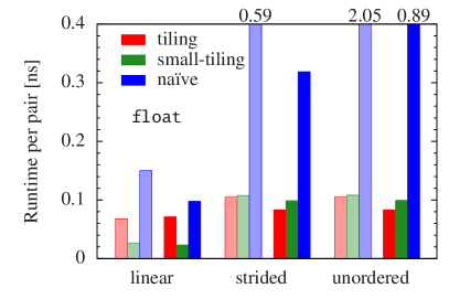
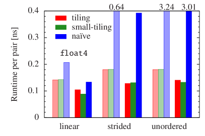
Figure 7: Runtime performance of different $O\bigl{(}N^{2}\bigr{)}$-memory access patterns using various GPU implementations, see Algorithms 3 and 4. The figures show kernel execution times divided by the number of pairs, $N^{2}$, in the scaling limit of a large number of array elements, $N$. The two panels compare arrays of data type float (left) and float4 (right). Light (left groups) and solid (right groups) fillings distinguish results for GPUs without and with hardware cache, respectively; see text for details. Some runtimes of the naïve implementation exceed the axis range and are printed at the top. Note that the total amount of transferred memory is larger by a factor of 4 for float4 values.

Runtime measurements were conducted on two systems with GPU hardware with and without on-chip memory cache. The first system hosted an Nvidia Tesla S1070 server (T10 chip, CUDA compute capability 1.3), and the second system contained four Tesla C2050 (“Fermi”) cards (compute capability 2.0). The latter GPU is, among other improvements, equipped with a hardware cache of 48 kB. For both systems, we used the same kernel builds created by the CUDA SDK version 3.2 with the compilation option –arch sm_12. Kernels were run with 128 threads per block on a single GPU; kernel execution times were averaged over 100 repetitions and do not include data transfer from host to GPU memory. The array size was varied between $N=1{,}000$ and 70,000 checking that the runtime divided by $N^{2}$ has converged, and the obtained runtimes are presented in Fig. 7.

The runtime of the naïve implementation depends sensitively on the access pattern, which nicely illustrates the effect of the hardware cache. In the absence of a cache and for arrays of data type float, the kernel with unordered access is slower by a factor of 13 compared to the linear pattern; this reduces to 9 on the C2050 card. The factor, however, increases from 15 (S1070) to 23 (C2050) if the basic data type is float4 (16 bytes per array element). Keeping the access pattern and the data type fixed, the largest observed runtime improvement was by a factor of 2.3 for unordered access and float data, which we mainly attribute to the presence of memory cache and the higher number of multiprocessors on the C2050 GPU. The overall observation of a higher performance gain using the latter hardware for float data is likely due to the fact that the cache can store simply more float than float4 data items, reducing the number of cache misses upon later access of the same data by another thread.

The two tiling algorithms are between 1.3 (linear access) to 20 times (unordered access) faster than their respective naïve implementations. Both algorithms exhibit similar execution times, they are even comparable for the different access patterns, solely the linear access is somewhat faster. This shows that manual caching via shared memory can efficiently hide even complex memory access. Comparing the two GPU generations, the C2050 is found to be slightly more efficient for float4 data, but to perform similarly as one of the S1070 GPUs for float. A notable exception is linear access to float data, where the “small-tiling” implementation is about 2–3 times faster than the original tiling algorithm CUD (2010); Nyland et al. (2007). The advantages of the “small-tiling” version are expected to become relevant only for larger array elements (e.g., 2 × float4), when the considerations on shared memory and multiprocessor occupancy given in Section 3 apply.

Summarising, the built-in memory cache of the Tesla C2050 hardware yields significant improvements to global memory access with the straightforward, “naïve” implementation of our test kernels. In particular, this implementation performs well for linear access of float4 data in the presence of a hardware cache. It can, however, not compete with an explicit caching algorithm via shared memory, which can be designed to reflect the actual data processing scheme for optimal cache efficiency and coalescable memory transfer. The “small-tiling” algorithm achieves in all test cases a high memory transfer bandwidth and seems to be rather robust with respect to access patterns and sizes of the array elements. It may be worth to investigate whether it can speed up matrix-vector multiplications, where the data of the vector are linearly read by all threads.

References

- Franosch et al. (2011) T. Franosch, M. Grimm, M. Belushkin, F. M. Mor, G. Foffi, L. Forro, and S. Jeney, Nature 478, 85 (2011).
- Lutz et al. (2006) C. Lutz, M. Reichert, H. Stark, and C. Bechinger, Europhys. Lett. 74, 719 (2006).
- Wysocki et al. (2009) A. Wysocki, C. P. Royall, R. G. Winkler, G. Gompper, H. Tanaka, A. van Blaaderen, and H. Löwen, Soft Matter 5, 1340 (2009).
- Milinkovic et al. (2011) K. Milinkovic, J. T. Padding, and M. Dijkstra, Soft Matter 7, 11177 (2011).
- Rinn et al. (1999) B. Rinn, K. Zahn, P. Maass, and G. Maret, Europhys. Lett. 46, 537 (1999).
- Bleibel et al. (2011) J. Bleibel, S. Dietrich, A. Domínguez, and M. Oettel, Phys. Rev. Lett. 107, 128302 (2011).
- Dünweg and Ladd (2009) B. Dünweg and A. Ladd, in Advanced Computer Simulation Approaches for Soft Matter Sciences III, edited by C. Holm and K. Kremer (Springer Berlin/Heidelberg, 2009), vol. 221 of Advances in Polymer Science, pp. 89–166, ISBN 978-3-540-87705-9.
- Gompper et al. (2009) G. Gompper, T. Ihle, D. Kroll, and R. Winkler, in Advanced Computer Simulation Approaches for Soft Matter Sciences III, edited by C. Holm and K. Kremer (Springer Berlin/Heidelberg, 2009), vol. 221 of Advances in Polymer Science, pp. 1–87, ISBN 978-3-540-87705-9.
- Padding and Louis (2006) J. T. Padding and A. A. Louis, Phys. Rev. E 74, 031402 (2006).
- Ermak and McCammon (1978) D. L. Ermak and J. A. McCammon, J. Chem. Phys. 69, 1352 (1978).
- Durlofsky et al. (1987) L. Durlofsky, J. F. Brady, and G. Bossis, J. Fluid Mech. 180, 21 (1987).
- Banchio and Brady (2003) A. J. Banchio and J. F. Brady, J. Chem. Phys. 118, 10323 (2003).
- Ladd (1993) A. J. C. Ladd, Phys. Fluids A 5, 299 (1993).
- Padding and Louis (2004) J. T. Padding and A. A. Louis, Phys. Rev. Lett. 93, 220601 (2004).
- Putz et al. (2010) V. B. Putz, J. Dunkel, and J. M. Yeomans, Chem. Phys. 375, 557 (2010).
- Baker and Hirst (2011) J. A. Baker and J. D. Hirst, Mol. Inform. 30, 498 (2011).
- Anderson et al. (2008) J. A. Anderson, C. D. Lorenz, and A. Travesset, J. Comp. Phys. 227, 5342 (2008).
- van Meel et al. (2008) J. A. van Meel, A. Arnold, D. Frenkel, S. Portegies Zwart, and R. G. Belleman, Mol. Simul. 34, 259 (2008).
- Colberg and Höfling (2011) P. H. Colberg and F. Höfling, Comput. Phys. Commun. 182, 1120 (2011).
- Ruymgaart et al. (2011) A. P. Ruymgaart, A. E. Cardenas, and R. Elber, J. Chem. Theory Comput. 7, 3072 (2011).
- Röhm and Arnold (2012) D. Röhm and A. Arnold, Eur. Phys. J. Special Topics (2012), in this issue.
- Batchelor (2000) G. Batchelor, An introduction to fluid dynamics, Cambridge mathematical library (Cambridge University Press, 2000), ISBN 9780521663960.
- Dhont (1996) J. K. G. Dhont, An introduction to dynamics of colloids (Elsevier, 1996), 2nd ed.
- Eckhardt and Buehrle (2008) B. Eckhardt and J. Buehrle, Eur. Phys. J. Special Topics 157, 135 (2008).
- Oseen (1927) C. W. Oseen, Neuere Methoden und Ergebnisse in der Hydrodynamik (Akad. Verlagsges., Leipzig, 1927).
- Mazur and van Saarloos (1982) P. Mazur and W. van Saarloos, Physica A 115, 21 (1982).
- Rotne and Prager (1969) J. Rotne and S. Prager, J. Chem. Phys. 50, 4831 (1969).
- Cox (1974) R. Cox, Int. J. Multiphase Flow 1, 343 (1974).
- Jeffrey and Onishi (1984) D. J. Jeffrey and Y. Onishi, J. Fluid Mech. 139, 261 (1984).
- Ladd (1990) A. J. C. Ladd, J. Chem. Phys. 93, 3484 (1990).
- CUD (2010) NVIDIA CUDA C Programming Guide (2010), version 3.2.
- Nyland et al. (2007) L. Nyland, M. Harris, and J. Prins, in GPU Gems 3, edited by H. Nguyen (Addison Wesley, 2007), chap. 31.
- Colberg and Höfling (2008–2012) P. H. Colberg and F. Höfling, Highly Accelerated Large-scale Molecular Dynamics package (2008–2012), http://halmd.org.
- Tory et al. (1991) E. Tory, M. Kamel, and C. Tory, Powder Technol. 67, 71 (1991).
- Nguyen and Ladd (2002) N.-Q. Nguyen and A. J. C. Ladd, Phys. Rev. E 66, 046708 (2002).
- Pham et al. (2009) T. T. Pham, U. D. Schiller, J. R. Prakash, and B. Dünweg, J. Chem. Phys. 131, 164114 (2009).
- Sierou and Brady (2001) A. Sierou and J. F. Brady, J. Fluid Mech. 448, 115 (2001).
- Bédorf et al. (2012) J. Bédorf, E. Gaburov, and S. P. Zwart, J. Comp. Phys. 231, 2825 (2012).
- Bédorf and Zwart (2012) J. Bédorf and S. P. Zwart, Eur. Phys. J. Special Topics (2012), in this issue.