Modified perturbation theory for angular distribution in $W$-pair production

Abstract

We examine the capabilities of the modified perturbation theory (MPT) for description of $W$-pair production and decay in $e^{+}e^{-}$ annihilation. In a model with Dyson-resummed propagators of unstable particles, we calculate even and odd contributions to the distribution in the cosine of the $W^{-}$ production angle relative to the $e^{-}$ beam. On comparing the results of calculations in the NNLO approximation of MPT with the exact results in the model, a coincidence of outcomes at the ILC energies is detected at the per-mille level.

1 Introduction

Among the propositions for research at International Linear collider (ILC) [1], a significant place is assigned to measurements of interactions amongst gauge bosons. The problem of particular importance is the search for anomalous contributions to triple gauge couplings. The latter topic could become the most important issue in high energy physics if a light Higgs and supersymmetric particles would not be discovered.

The primary tool for measuring the triple gauge boson vertices is the study of angular distributions of $W$ bosons in the processes of $W$-pair production. At the ILC a few million of $W$ pairs is assumed to be produced at $\sqrt{s}=500$ GeV and 800 GeV [1, 2]. This implies that the cross-section and various integral characteristics of angular distributions of $W$ bosons may be determined at the per-mille level. (Under the integral characteristics we mean quantities used in the method of optimal observables [3, 4] or $\chi^{2}$ fit over a wide range of the phase space [5].) The anomalous contributions to triple gauge couplings are expected to be determined with similar precision [2, 3, 4, 5]. So, the theoretical calculation of the angular distribution must be made with the per-mille precision, too. This implies the next-to-next-to-leading order (NNLO) accuracy of the calculations, at least, on the resonant contributions of $W$ bosons. Simultaneously the strict observance of the gauge cancellations must be maintained. The latter requirement in particular is critical in view of large gauge cancellations owing to which the $W$-pair production is notably sensitive to triple gauge couplings.

Unfortunately, there is a lack of calculation methods satisfying all mentioned requirements. For instance, the double pole approximation (DPA) successfully applied at LEP2 [6] can provide only the NLO accuracy of calculations and in the resonant region of the cross-section only. The complex mass scheme (CMS) [7] provides the NLO accuracy at higher energies, but the NLO is not sufficient for support of all potentialities at ILC. So a more powerful scheme is required which would allow one to consistently involve the NNLO in the calculations.

A probable candidate for such scheme is a modified perturbation theory (MPT) [8, 9, 10]. Its main feature is the direct expansion of the probability instead of amplitude in powers of the coupling constant with the aid of distribution-theory methods. The latter methods permit to impart a well-defined meaning to the resonant contributions of unstable particles in the expanded probability. A condition of asymptoticity (and therefore of completeness) of the expansion must ensure the gauge cancellations. In the case of pair production of unstable particles, the most-elaborated description of the method is given in [10]. In [11, 12] the convergence properties of the MPT expansion for the total cross-section were tested in models related to the top-quark-pair and $W$-pair production. (The models were based on the “improved” Born approximation and the Dyson resummation up to three loops of the resonant contributions of unstable particles.) In both cases a good convergence of the MPT series was detected at the ILC energies. In the case of the $W$-pair production, the precision of the NNLO approximation was observed at the level better than one per-mille [12].

In this paper we consider angular distribution of the $W^{-}$ boson relative to the direction of the $e^{-}$ beam in the center-of-mass frame. Actually this distribution is used in the experimental analysis of the triple gauge couplings. In fact the distribution is analysed together with changing the beam polarization in order to disentangle contributions from $\gamma WW$ and $ZWW$ vertices. From standpoint of the MPT, the changing of the polarization manifests itself as the changing of test function. However a variation of the test function has virtually no effect on the convergence of the MPT series [11, 12] provided that the set of singularities arising in the MPT is unchanged. The set of singularities is invariable in the cases of even and odd contributions to the distribution in the cosine of the $W$ production angle. So for the analysis of the convergence properties of the MPT series, we may confine ourselves to consideration separately of the even and odd contributions and in the case of unpolarized beams only. By these means we would be able to verify the convergence properties of the MPT expansion simultaneously for wide variety of beam polarizations.

The paper is organized as follows. In Sec. 2, we consider specifics of the MPT in the case of the angular distribution and determine a method of handling new-type singularities that arise in this case in the framework of the MPT. In Sec. 3, we present results of numerical calculations. In Sec. 4, we discuss results and make conclusions.

2 MPT for angular distribution

The angular distribution of $W$-pair production in $e^{+}e^{-}$ annihilation has the form of a convolution of hard-scattering contributions with the flux function describing initial state radiation,

$${\cal D}\sigma(s,\cos\theta)=\int_{s_{\mbox{\tiny min}}}^{s}\frac{\mbox{d}s^{\prime}}{s}\>\phi(s^{\prime}/s;s)\>{\cal D}\hat{\sigma}(s^{\prime},\cos\theta)\,.$$ (1)

Here ${\cal D}=\mbox{d}/\mbox{d}\cos\theta$, $\theta$ is the $W^{-}$ production angle relative to the $e^{-}$ beam in the rest frame, $\phi$ is the flux function. The hard-scattering contributions ${\cal D}\hat{\sigma}$ are described as an integral of exclusive angular distribution over the virtualities of $W$ bosons,

$${\cal D}\hat{\sigma}(s^{\prime},\cos\theta)\;=\int^{\infty}_{{\displaystyle\mbox{\scriptsize$s$}}_{1\mbox{\tiny min}}}\int^{\infty}_{{\displaystyle\mbox{\scriptsize$s$}}_{2\mbox{\tiny min}}}\mbox{d}s_{1}\,\mbox{d}s_{2}\;\left(1+\delta_{soft}\right)\,{\cal D}\hat{\sigma}_{ex}(s^{\prime},\cos\theta\,;s_{1},s_{2})\,.$$ (2)

In this formula $s_{1\,\mbox{\scriptsize min}}$ and $s_{2\,\mbox{\scriptsize min}}$ are the minimum virtualities, $\sqrt{s_{\mbox{\scriptsize min}}}=\sqrt{s_{1\,\mbox{\scriptsize min}}}+\sqrt{s_{2\,\mbox{\scriptsize min}}}$, $\delta_{soft}$ stands for factorized contributions of soft massless particles. The exclusive contribution, in turn, is written as a product of Breit-Wigner (BW) factors $\rho(s_{i})$, some kinematic factors, and a function $\Phi$ which is the rest of the amplitude squared,

$$\hat{\sigma}_{ex}(s,\cos\theta\,;s_{1},s_{2})=\Theta(\!\sqrt{s}-\!\sqrt{s_{1}}-\!\sqrt{s_{2}}\,)\sqrt{\lambda(s,\!s_{1},\!s_{2})}\;\Phi(s,\cos\theta\,;s_{1},s_{2})\,\rho(s_{1})\rho(s_{2})\,.$$ (3)

Here $\lambda(s,\!s_{1},\!s_{2})=(s-\!s_{1}\!-\!s_{2})^{2}-4s_{1}s_{2}$, and $\Theta(\dots)$ is the step function. Function $\Phi$ corresponds to one-particle irreducible contributions in the channels of $W$ bosons. Therefore it has no singularities on the mass-shell. As a first approximation, we regard that $\Phi$ is an analytic function and has no singularities. (By this we mean that the appropriate singularities are to be considered on the fact they are identified.) On the contrary, the kinematic factor, which is the product of the step function and the square root of the kinematic function, explicitly has singularities. The BW factors, if we naively expand them in powers of the coupling constant, generate non-integrable singularities.

However, the singularities might be made integrable if we expand the BW factors in the sense of distributions [13]. Actually, this is a basic idea of the MPT approach [8]. In this case the expansion of a separately taken BW factor is beginning with the $\delta$-function, which corresponds to the narrow-width approximation. The contributions of the naive Taylor expansion are supplied with the principal-value prescription for the poles. The nontrivial contributions are the delta-function and its derivatives with coefficients $C_{n}$, which are polynomials in the coupling constant $\alpha$ and which correct the contributions of the Taylor. Within the NNLO, the expansion looks as follows [10]:

$$\displaystyle\rho(s)\;\;\equiv\;\;\frac{M\Gamma_{0}}{\pi}\;{|s-M^{2}+\Sigma(s)|^{-2}}\;\;=\;\;\delta(s\!-\!M^{2})$$ (4)

$$\displaystyle+\;\frac{M\Gamma_{0}}{\pi}\,PV\!\left[\,\frac{1}{(s-M^{2})^{2}}-\frac{2\alpha\,\mbox{Re}\Sigma_{1}(s)}{(s\!-\!M^{2})^{3}}\,\right]+\sum\limits_{n\,=\,0}^{2}C_{n}(\alpha)\,\delta^{(n)}(s\!-\!M^{2})+O(\alpha^{3})\,.$$

Here $PV$ is the principal-value prescription, $M$ is the renormalized mass of the unstable particle, $\Gamma_{0}$ is its Born width, $\alpha\,\Sigma_{1}(s)$ is the one-loop self-energy. Within the NNLO in OMS-like schemes of UV renormalization, coefficients $C_{n}(\alpha)$ include three-loop self-energy contributions and their first derivatives determined on-shell.

Unfortunately, the above expansion is senseless if the weight at the expansion is not smooth enough. In formula (3) the weight is not smooth because of singular behavior of the kinematic factor. So, the next ingredient of the MPT is the analytic regularization of the kinematic factor via the substitution $[\lambda(s,s_{1},s_{2})]^{1/2}\to[\lambda(s,s_{1},s_{2})]^{\nu}$ [10]. The rest of the weight is represented in the form of Taylor expansion in variables $s_{1}$ and $s_{2}$ around the mass-shell, with a remainder. The integrals of the remainder may be numerically calculated without the regularization. The integrals of Taylor are reduced to the sum of basic integrals, which may be analytically calculated irrespective of details of definition of the weight. In the end with $\nu=1/2$ this gives finite outcomes in any order in the expansion in powers of $\alpha$ and the expansion remains asymptotic [10].

When calculating the total cross-section with $\Phi$ determined in the Born approximation, this scheme works well [12]. However in the case of the angular distribution a non-analyticity in $\Phi$, related to neutrino propagator in the $t$-channel, becomes relevant. Namely, the square root of the kinematic function $\lambda$ in the denominator of the propagator becomes relevant,

$$\Delta_{\nu}\;=\;\frac{1}{s-s_{1}-s_{2}-\sqrt{\lambda}\,\cos\theta}\;\sim\;\frac{1}{t_{\nu}}\,.$$ (5)

Note that in the total cross-section, the integrating d$\cos\theta$ results in an entire function of $\lambda$ in the vicinity of $\lambda=0$. But in the case of angular distribution the $\sqrt{\lambda}$ persists. Of course, the $\sqrt{\lambda}$ may be analytically regularized by means of the substitution $\sqrt{\lambda}\to\lambda^{\nu}$. However, when calculating the Taylor series, this leads to a growth of singularity, which considerably complicates calculations.

An alternative way is to represent propagator (5) in an equivalent form with an entire function in the denominator,

$$\Delta_{\nu}\;=\;\frac{s-s_{1}-s_{2}+\sqrt{\lambda}\,\cos\theta}{(s-s_{1}-s_{2})^{2}-\lambda\,\cos^{2}\theta}\,.$$ (6)

Then, function $\Phi$ may be considered as a sum of two contributions, one with integer powers of $\lambda$ and another with an additional factor $\sqrt{\lambda}$ in the numerator. The former contribution is handled by the above scheme. In the latter contribution we remove the additional $\sqrt{\lambda}$ in $\Phi$ in favour of the kinematic factor, so that the kinematic factor would include $\lambda^{\nu+1/2}$ instead of $\lambda^{\nu}$.

Further let us remember that the contributions of the above-mentioned Taylor expansion are expressed in terms of the basic integrals $I^{\nu}_{n}$, $J^{\nu}_{n}$, $A^{\nu}_{n_{1},n_{2}}$, $B^{\nu}_{n_{1},n_{2}}$, and $C^{\nu}_{n_{1},n_{2}}$. (In fact $C^{\nu}_{n_{1},n_{2}}$ is represented as a sum of other basic integrals and a regular function. For this reason we do not discuss $C^{\nu}_{n_{1},n_{2}}$ below.) In the original work [10] the basic integrals were calculated at non-integer $\nu$, and only half-integer $\nu$ was needed in the final stage with smooth $\Phi$. At the same time, a transition to integer $\nu$ was not obvious because of singular behavior of some factors. However, the transition is possible through asymptotic expansion of singular factors. The mentioned factors are the $\Gamma$-function whose argument tends to negative integer or zero, and the distribution $x_{+}^{\beta}$ with $\beta$ tending to negative integer. Their asymptotic expansions are as follows:

$$\Gamma(\,1-N+\varepsilon)=\frac{1}{\varepsilon}\,\frac{(-)^{N-1}}{(N-1)!}\,+\,O(1)\,,$$ (7)

$$x^{-N+\varepsilon}_{+}=\frac{1}{\varepsilon}\,\frac{(-)^{N-1}}{(N-1)!}\;\delta^{(N-1)}(x)\,+\,x_{+}^{-N}\,+\,O(\varepsilon)\,.$$ (8)

Here $N=1,2,\,\dots$ , and $x_{+}^{-N}$ is the adjoint distribution of the 1-st order [13]. Fortunately the $x_{+}^{-N}$ does not appear in the final formulas owing to the relation

$$x_{+}^{-N}+(-)^{-N}(-x)_{+}^{-N}=PVx^{-N}\,.$$ (9)

It is worth to recall that the asymptotic expansion in (8) is defined in the sense of distributions, which means that both sides of the relation are to be integrated with smooth enough weight.

Formulas (7)-(9) are sufficient for the determination of the basic integrals with non-negative integer $\nu$. The basic integrals needed within the NNLO are as follows:

$${\tt I}^{\,1}_{1}(x)=x_{+}\,,$$ (10)

$$\displaystyle{\tt J}^{\,1}_{1}(x|a_{i}) = -(x+a_{i})_{+}\!+\Theta(x+a_{i})\,x\ln\!\frac{|x|}{a_{i}}\,,$$ (11)

$${\tt J}^{\,1}_{2}(x|a_{i}) = -\frac{1}{a_{i}}(x+a_{i})_{+}\!-\Theta(x+a_{i})\ln\!\frac{|x|}{a_{i}}\,,$$

$$A^{\,1}_{1\,1}=x_{+}\,,\quad A^{\,1}_{1\,2}=A^{\,1}_{2\,1}=-\Theta(x)\,,\quad A^{\,1}_{1\,3}=A^{\,1}_{3\,1}=\frac{1}{2}\,\delta(x)\,,\quad A^{\,1}_{2\,2}=\delta(x)\,,$$ (12)

$$B^{\,1}_{1\,1}(x|a_{i}) \equiv \bar{B}^{\,1}_{1\,1}(x|a_{i})\,\>=\>\,{\tt J}^{\,1}_{1}(x|a_{i})\,,$$ (13)

$$B^{\,1}_{2\,1}(x|a_{i}) \equiv \bar{B}^{\,1}_{2\,1}(x|a_{i})\,\>=\>\,{\tt J}^{\,1}_{2}(x|a_{i})\,.$$

Here $x$ is dimensionless variable associated with $s$ by the relation $x=2M^{-1}(\sqrt{s}-2M)$, and $a_{i}$ are dimensionless parameters, $a_{i}=2M^{-1}(M-\sqrt{s_{i\,\mbox{\scriptsize min}}})$.

Another problem arising at calculating the angular distribution is connected with zeros in the denominator in (6). Actually, the denominator is nulled at $s-s_{1}-s_{2}=0$ and $\cos\theta=0$. The former equality implies $\lambda<0$, which means non-physical region. However, the Taylor expansion of the weight effectively means extension into non-physical region. Really, with small enough $s$ one of $s_{i}$, or both $s_{1}$ and $s_{2}$, are taken due to the Taylor on the mass-shell. As a result, the denominator in (6) affects the calculations with $s-s_{1}-s_{2}=0$. This means failure of the calculations at $\cos\theta=0$ and an instability of outcomes of calculations in the vicinity of $\cos\theta=0$.

The problem may be solved by redefinition of the denominator in the non-physical region so that it would be positive everywhere. So, by taking advantage of the identity

$$(s-s_{1}-s_{2})^{2}-\lambda\,\cos^{2}\theta\;=\;\lambda\,(1-\cos^{2}\theta)+4s_{1}s_{2}\,,$$ (14)

we represent (6) in the form

$$\Delta_{\nu}\;=\;\frac{s-s_{1}-s_{2}+\sqrt{\lambda}\,\cos\theta}{H(\lambda)\,(1-\cos^{2}\theta)+4s_{1}s_{2}}$$ (15)

with

$$H(\lambda)\;=\;\Theta(\lambda)\,\lambda\;+\;\Theta(-\lambda)\,h(\lambda)\,.$$ (16)

Here $h(\lambda)$ is a function that provides positivity of the denominator and, simultaneously, sufficient smoothness of the function $H(\lambda)$. Since within the NNLO the Taylor implies second-order derivatives, function $H(\lambda)$ must be continuous with its second derivatives. These conditions are satisfied, for instance, by

$$h(\lambda)=\lambda\left[1-\left(-\lambda/\lambda_{0}\right)^{n}\right]\,,$$ (17)

where $n\geq 2$, $0<\lambda_{0}<4\,s_{1\mbox{\scriptsize min}}\,s_{2\mbox{\scriptsize min}}\,(n\!+\!1)^{(n+1)/n}/n$.

We stress that the above procedure in no way affects the integrand (2) in the region of integration (in the physical region) and thus in no way affects the value of the integral itself. Nevertheless, the redefinition of the integrand in the extended region allows us to calculate the asymptotic expansion of the integral by means of asymptotic expansion of the BW factors and the Taylor expansion of the weight. The result of the calculation must be the same as that in the case of direct asymptotic expansion of the previously calculated integral.

Now we briefly discuss the physical model in which we carry out calculations. As mentioned in the Introduction, the model is the same that was used in [12]. It is based on the improved Born approximation in the Standard Model for the amplitude and the Dyson resummation up to three loops of the resonant contributions of unstable particles. The improved Born approximation implies taking into consideration the universal soft massless-particles contributions that are collected in the flux function $\phi$ and in the Coulomb factor in $\delta_{soft}$. We consider the flux function in the leading-log approximation, and the Coulomb factor in the one-photon approximation with specific resummation that does not affect the BW factors, see details and references in [10, 12].

The scalar part of the $W$-boson propagator in the model, we consider in the form:

$$\Delta^{-1}(s)\;\;=\;\;s\,-\,M^{2}\,+\,\alpha\,\mbox{Re}\Sigma_{1}(s)\,+\,\mbox{i}\,\alpha\,\mbox{Im}\Sigma_{1}(s)$$

$$+\;\alpha^{2}\left[R_{2}\,+\,\mbox{i}\,I_{2}\,+\,(s-M^{2})(R^{\prime}_{2}+\mbox{i}\,I^{\prime}_{2})\,\right]\>+\>\alpha^{3}\left(R_{3}+\mbox{i}\,I_{3}\right).$$ (18)

Here $R_{n}=\mbox{Re}\,\Sigma_{n}(M^{2})$, $I_{n}=\mbox{Im}\,\Sigma_{n}(M^{2})$, and the prime means derivatives. $\mbox{Re}\Sigma_{1}(s)$ and $\mbox{Im}\Sigma_{1}(s)$ can be determined by direct calculations, but for simplicity we restrict ourselves by considering quark and lepton contributions only. In this way we avoid the IR divergences. The on-shell self-energy contributions can be determined by means of the UV renormalization conditions and the conditions of unitarity. We use the $\overline{\mbox{OMS}}$ scheme [15, 16] of the UV renormalization, a natural generalization of the conventional OMS scheme for the case of unstable particles. In this scheme the imaginary contributions to on-shell self-energies are expressed through the Born-, one-loop, and two-loop contributions to the widths of the unstable particles.

Propagator (2) is considered as the exact one in the model. The MPT-expansion of the appropriate BW factors are determined by (4) with coefficients $C_{n}(\alpha)$ given in [10]. The definition of $\Phi$ in the Born approximation is straightforward except $Z$-boson propagator in the $s$-channel. Namely, at the resonant energies for the $Z$ boson, we define its propagator as was done in (2). So, when considering the model in the MPT-mode, we expand $Z$-boson propagator in the MPT sense. However, at high enough energies, we define Z-boson propagator to be free, thus preserving the gauge cancellations and the unitarity, see details in [12].

The angular distributions in the model are straightforwardly calculated. We calculate the case of unpolarized beams. The outcomes with the propagator (2), are called the “exact results in the model”. The angular distributions in the MPT-mode have the form ${\cal D}\sigma={\cal D}\sigma_{0}+{\cal D}\alpha\sigma_{1}+{\cal D}\alpha^{2}\sigma_{2}$, where $\sigma_{0}$ is the cross-section in the LO approximation, $\alpha\sigma_{1}$ and $\alpha^{2}\sigma_{2}$ are the NLO and NNLO corrections. So, ${\cal D}\sigma_{NLO}={\cal D}\sigma_{0}+{\cal D}\alpha\sigma_{1}$ and ${\cal D}\sigma_{NNLO}={\cal D}\sigma_{0}+{\cal D}\alpha\sigma_{1}+{\cal D}\alpha^{2}\sigma_{2}$ determine the NLO and NNLO approximations, respectively.

3 Numerical results

For numerical calculations, we use the same values of kinematic and model parameters and the same parametrization that was used in [12]. The outcomes of the calculations are presented at the typical ILC energies $\sqrt{s}=500$ GeV and $\sqrt{s}=800$ GeV [1, 2].

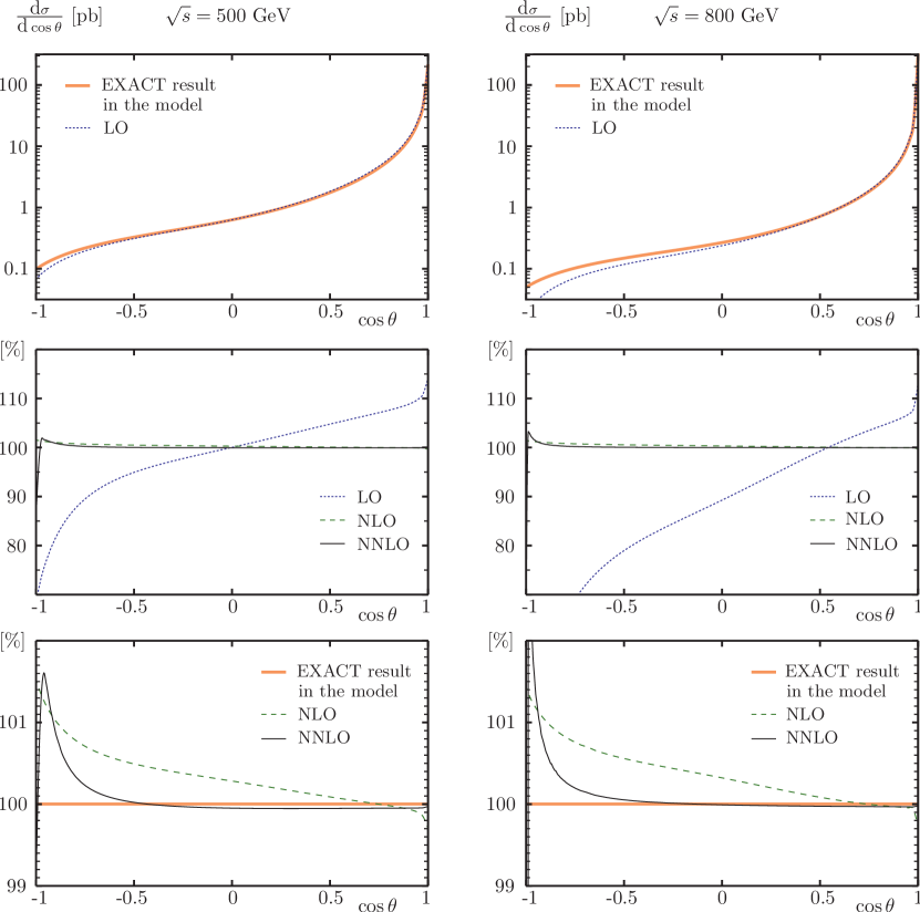
Figure 1: Distribution in the cosine of the $W^{-}$ production angle relative to the $e^{-}$ beam in $e^{+}e^{-}\to\gamma,Z\to W^{+}\>W^{-}\to 4f$ at $\sqrt{s}=500$ GeV (l.h.s.) and $\sqrt{s}=800$ GeV (r.h.s) in the case of unpolarized beams. In the upper row, the exact result in the model and the result in the LO in the MPT are shown. At the middle and lower row, the percentages of the results in the LO, NLO, and NNLO approximations in the MPT with respect to the exact result are shown.

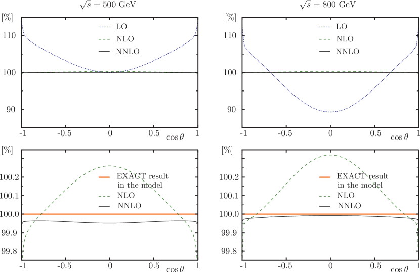
Figure 2: The MPT results in percentage with respect to the exact result for the even contribution to the $\cos\theta$-distribution.

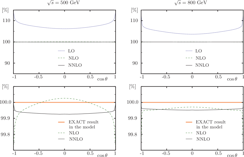
Figure 3: The MPT results in percentage with respect to the exact result for the odd contribution to the $\cos\theta$-distribution.

In Figs. 1$-$3 we present the full $\cos\theta$-distribution, and separately the even and odd contributions, respectively. In all figures the thick curves show the exact result in the model. The dotted, dashed, and thin continuous curves show the results in the LO, NLO, and NNLO approximations in the MPT, respectively. The curves for the NLO and NNLO are omitted in the upper row in Fig. 1, since they merge with the curves for the exact result at a given scale. Instead, they are shown in the middle and lower rows, where the percentages with respect to the exact result are presented. In Fig. 2 and 3, we omit “upper row” with the absolute-value results for the even and odd contributions in view of their minor informativity, and present only percentages of the corresponding approximations relative to the appropriate exact results. In all figures the lowest row repeats the results of the preceding row with greater scale on vertical axis.

Examining the figures, we note first and foremost a stable behavior of the NLO approximation and more stable behavior of the NNLO approximation in the cases of even and odd contributions (Figs. 2 and 3, respectively). The accuracy of the NLO approximation in these cases is within a few per-mille and that of the NNLO approximation persistently is better than one per-mille. In the case of the full angular distribution (Fig. 1) the picture generally is the same except the region of $\cos\theta$ approaching $-1$. In the latter region the even and odd contributions almost cancel each other, thus giving in the sum a substantially reduced outcome. For instance, with $\cos\theta=-0.95$ the outcome is diminished by about two orders of magnitude: ${\cal D}\sigma=12.72-12.59\simeq 0.12$ pb and ${\cal D}\sigma=5.574-5.513=0.061$ pb for $\sqrt{s}=500$ GeV and 800 GeV, respectively. As a result, a discrepancy of the sum increases near $\cos\theta=-1$. The tendency is as follows: with $\cos\theta=0.95$ at $\sqrt{s}$ = 500(800) GeV the discrepancy in the NNLO approximation makes up 0.05(0.03)%; with $\cos\theta=-0.64(-0.63)$ the discrepancy overcomes the level of 0.1%; with $\cos\theta=-0.95$ the discrepancy makes up 1.4(1.5)%. The latter values are to be compared with the discrepancies for the even and odd contributions taken separately, which are 0.04(0.02)% and 0.05(0.04)%, respectively, and with two orders of magnitude cancelled in the full $\cos\theta$-distribution.

It should be remembered that with $\cos\theta$ approaching $-1$ the quality of the experimental data in the case of unpolarized beams becomes worse, too. This occurs because of the smallness the values of the angular distribution and therefore its statistical significance decreases, and also because of the increasing background [5]. So the effect of decreasing the accuracy of the MPT description most likely will not spoil quality requirements in this region. On the other hand, with polarized beams the angular distribution must become more noticeable at $\cos\theta\simeq-1$. In particular, with purely right-polarized $e^{-}$ beam the odd contribution disappears. Therefore the very reason for the above mentioned cancellations disappears, too. So, in general, in most cases of beams polarization there should be no peaks in the region of backward-scattering in the percentage distributions of the MPT description.

In the end of this Section it is worth noticing that the above mentioned effect of decreasing accuracy of the MPT description in the case of unpolarized beams and large backward scattering angles does not appear at all in the cases of the total cross-section and the forward-backward asymmetry $A_{FB}$. Really, the total cross-section is determined as the integral $\mbox{d}\cos\theta$ of the $\cos\theta$-distribution in symmetric limits, so only the even contribution is relevant. Therefore, the accuracy of the description of the total cross-section in the NNLO is better than one per-mille at the ILC energies [12]. The forward-backward asymmetry $A_{FB}$ is determined as the ratio of the integral of the odd contribution to the integral of the even contribution to $\cos\theta$-distribution. Therefore, the accuracy of the description of $A_{FB}$ is within one per-mille, as well. The numerical results at the characteristic ILC energies are presented in Table 1.

Table 1: Results of MPT calculations for forward-backward asymmetry $A_{FB}$.

$\quad\sqrt{s}$ (MeV)	$\quad\;A_{FB}^{\,\mbox{\tiny EXACT}}\quad\;$	$\qquad A_{FB}^{LO}\quad\;$	$\quad\;A_{FB}^{NLO}\qquad$	$\quad A_{FB}^{NNLO}\qquad$
500	0.9025	0.9150	0.9011	0.9022(1)
	100%	101.38%	99.94%	99.96(1)%
800	0.9207	0.9409	0.9202	0.9204(1)
	100%	102.19%	99.95%	99.97(1)%

The numbers in parenthesis in the last column show uncertainties in the last digits due to computations. In other columns the uncertainties are omitted as they are beyond the precision of the presentation of data. The algorithm for estimating the uncertainties is described in [17].

4 Discussion and conclusions

We have tested the applicability of the MPT in the case of angular distribution of $W$ bosons in the processes of $W$-pair production in $e^{+}e^{-}$ annihilation. Specifically, in a model that admits exact solution, we have calculated separately the even and odd contributions to the distribution in the cosine of the $W^{-}$ production angle relative to the $e^{-}$ beam. At the ILC energies a coincidence of the MPT outcomes with the exact result is detected within a few per-mille in the NLO approximation, and within one per-mille in the NNLO approximation.

In fact, despite the results of previous investigations of the total cross-section [12], the accuracy of the MPT-description in the case of angular distribution a priori was not known because of the presence of new-type singularities in the odd contribution to the $\cos\theta$-distribution. Such singularities were missed in previous MPT investigations. Initially they arise from the $t$-channel neutrino exchange and then they give rise to logarithmic and delta-function singularities in the exclusive cross-section, in addition to the power-like singularities in the general case [10]. (Recall that in the observable cross-section all singularities are integrated out.) Another novelty in the present calculations is a trick permitting to avoid spurious singularities arising in the non-physical momentum region involved in the MPT calculations. The mentioned trick enriches the set of techniques in the approach of MPT.

Actually, we have carried out calculations in the case of unpolarized beams only. However, the results may easily be generalized to cases with different polarizations. This is possible due to intrinsic property of the MPT, which is the almost independence of the results expressed in the relative units from smooth variation of the test function (i.e. without the occurrence of new singularities). This property is quite natural from the standpoint of theory of distributions where the distributions are considered as continuous linear functionals acting on linear space of test functions [13]. In the MPT this property was explicitly verified [11, 12]. It permits to extend the result concerning the accuracy of the MPT description to cases with different polarizations. Really, a change of the polarization means smooth variations of the test functions for the even and odd contributions to the $\cos\theta$-distribution. Owing to smoothness of the variations, the accuracy of the MPT description of the even and odd contributions must remain at the same level.

An important corollary of this result is that the accuracy of the description of the full angular distribution must remain at the same level, i.e. at the level of one per-mille in the NNLO approximation. (Let us recall that this is the accuracy that is required at the ILC.) The only exception is the case of large cancellations between the even and odd contributions, what happens in the case of unpolarized beams in the region of large backward scattering angles. In this region the accuracy in relative units is decreasing following the scale of the cancellation in the full angular distribution. However, owing to diminishing the signal the quality of experimental data becomes worse, too. So it is unlikely that the mentioned effect would be crucial when extracting information from experimental data. At the same time, in most cases of beams polarization when there are no large cancellations and therefore the angular distribution is not too small, the accuracy of the MPT description in the NNLO must remain at the per-mille level throughout.

To conclude the discussion, two more comments are in order. First, owing to the almost independence of the results of MPT calculations expressed in relative units from particular form of the test function, the turning on of the loop correction to the amplitude should not lead to noticeable modification of our results concerning the precision of MPT calculations. Notice this remark should be in force also because all types of basic singularities that can appear in the hard-scattering cross-section have been taken into consideration in our analysis (the power-like, logarithmic, and delta-function). The second remark concerns the single-resonant and interference contributions. Actually this issue was discussed earlier [10], and it was shown that such contributions may be taken into consideration precisely by the same technique as discussed above. So in these cases our results about the precision of the MPT-description must be in force, as well.

In summary, the MPT in the NNLO approximation gives on the whole satisfactory (from standpoint of ILC) results for the angular distribution of $W$ bosons in the processes of $W$-pair production and decay in $e^{+}e^{-}$ annihilation. On this basis and taking into consideration the preceding results for the total cross-section [12], we conclude that the MPT is really a good candidate for theoretical support at the ILC of the processes of $W$-pair productions.

References

- [1] G. Aarons, et al., ILC Reference Design Report Volume 2: Physics At The ILC, arXiv:0709.1893.
- [2] G. Moortgat-Pick et al., Phys. Rept. 460 (2008) 131.
- [3] M. Diehl, O. Nachtmann, F. Nagel, Eur. Phys. J. C 27 (2003) 375.
- [4] M. Diehl, O. Nachtmann, F. Nagel, Eur. Phys. J. C 32 (2003) 17.
- [5] W. Menges, A Study of Charged Current Triple Gauge Couplings at TESLA, LC-PHSM-2001-022.
- [6] M. Grunewald et al., Reports of the Working Groups on Precision Calculations for LEP2 Physics: Proceedings. Four fermion production in electron positron collisions, arXiv:hep-ph/0005309.
- [7] A. Denner, S. Dittmaier, M. Roth, L.H. Wieders, Nucl. Phys. B 724 (2005) 247.
- [8] F.V. Tkachov, in: Ya.I. Azimov, et al. (Eds.), Proc. 32nd PNPI Winter School on Nuclear and Particle Physics, St. Petersburg, PNPI, 1999, p. 166, arXiv:hep-ph/9802307
- [9] M.L. Nekrasov, Eur. Phys. J. C 19 (2001) 441.
- [10] M.L.Nekrasov, Int. J. Mod. Phys. A 24 (2009) 6071.
- [11] M.L. Nekrasov, Mod. Phys. Lett. A 26 (2011) 223.
- [12] M.L. Nekrasov, Mod. Phys. Lett. A 26 (2011) 1807.
- [13] I.M. Gelfand and G.E. Shilov, Generalized Functions, Academic Press, 1968
- [14] D. Bardin and T. Rieman, Nucl. Phys. B 462 (1996) 3.
- [15] M.L.Nekrasov, Plys. Lett. B 531 (2002) 225.
- [16] B.A. Kniehl, A. Sirlin, Phys. Lett. B 530 (2002) 129.
- [17] M.L. Nekrasov, PoS ACAT2010 (2010) 085.