An iterative domain decomposition method for free boundary problems with nonlinear flux jump constraint

Abstract

In this paper we design an iterative domain decomposition method for free boundary problems with nonlinear flux jump condition. Our approach is related to damped Newton’s methods. The proposed scheme requires, in each iteration, the approximation of the flux on (both sides of) the free interface. We present a Finite Element implementation of our method. The numerical implementation uses harmonically deformed triangulations to inexpensively generate finite element meshes in subdomains. We apply our method to a simplified model for jet flows in pipes and to a simple magnetohydrodynamics model. Finally, we present numerical examples studying the convergence of our scheme.

1 Introduction

In this paper, we propose a numerical iterative method for approximating the solutions of free boundary problems in two dimensions. Our iterative method for free boundary problems is based on Domain Decomposition and damped Newton’s method ideas. In general terms, free boundary problems seek to determine unknown function $u$ with some prescribed conditions on a unknown interior interface, exterior boundary or (sub)domain. In many applications, it is prescribed the value of $u$ on the free interface and it is required that $u$ satisfy a condition involving (both sides) derivatives of $u$ on the interface. We mention jump conditions of Stefan, Bernoulli and Gibbs-Thomson type, among others. There is a considerable literature of iterative methods for these type of free boundary problems; see for instance [4, 7, 8, 13, 14, 20, 22] and references therein. In particular, numerical finite elements methods have been proposed to solve Stefan-like free boundary problems (including time dependent problems) and some other similar phase transition problems; see for instance [3, 6, 15, 16, 19]. These methods use a variational formulation of their original problem. Level set approach for Stefan problems were also proposed in [5] and references therein.

The free boundary conditions that we deal with, up to our knowledge, have not been extensively studied from the numerical point of view. We are particularly interested in free boundary problems were the unknown function satisfy nonlinear jump constraints across the free interface. More precisely, given $\Omega\subset\mathbb{R}^{2}$, $g:\partial\Omega\to\mathbb{R}$ and $\lambda\in\mathbb{R}$, we want to find a function $u:\Omega\to\mathbb{R}$ and a free interface $\Gamma$ (diving $\Omega$ in two subdomains $\Omega^{+}=\{u>0\}$ and $\Omega^{-}=\{u<0\}$) such that $u$ and $\Gamma$ satisfy the following subdomain equations and boundary condition,

$$-\mbox{div}(a_{1}\nabla u)=0 \mbox{ in }~{}\Omega^{+},$$ (1)

$$-\mbox{div}(a_{2}\nabla u)=0 \mbox{ in }~{}\Omega^{-},$$ (2)

$$u=g \mbox{ on}~{}\partial\Omega$$ (3)

and free interface condition

$$a_{1}|\nabla u^{+}|^{2}-a_{2}|\nabla u^{-}|^{2}=\lambda~{}\mbox{on}~{}\Gamma,$$ (4)

or, similar nonlinear constraint for the jump in the derivative of $u$ across the free interface $\Gamma$. Above, $u^{+}$ and $u^{-}$ denote the value of the solution $u$ on both sides of the free interface and the derivatives and the quantities involved are interpreted as side limits. In many applications, the interface conditions are imposed in a weak sense. These conditions can be also interpreted if we replace the operators involved (e.g., trace of the derivatives) by some smooth or regularize version of them when necessary.

We are not aware of a simple inexpensive numerical method to solve problem (1)-(4). The finite element methods mentioned earlier to handle Stefan, Bernoulli and similar free boundary conditions are based on variational formulations. They do not seem to be easily extended to handle our nonlinear free boundary constraint. Also, Bernoulli type free boundary problems when one of the phases is a constant function seems to be easier to handle numerically. In this case, using the fact that the tangential derivative on the free interface is zero and that the flux sign can be a priori determined, the interface condition reduces to a linear condition of the form $\partial_{\eta}u=\lambda$ where $\partial_{\eta}$ is the normal derivative on the free interface.

We have two main applications in mind: 1) the jet flow model studied by Alt, Caffarelli, Friedman [2, 1] and 2) a free boundary problem arising in magnetohydrodynamics studied in [10, 12]. These applications are simplified mathematical versions of complicated flow models and they focus in the main modeling aspects. Despite of the mathematical simplifications, in either case, the resulting model problem above is still complex and finding and understanding solutions requires numerical methods. The methods used for this problems should be inexpensive and simple. The method presented here is designed having these considerations into account. It can also be easily extended to handle different free boundary problems such as the stationary solutions of the Stefan’s problem, and other similar problems.

The iterative method proposed in this paper for problem (1)-(4) is based on the following simple ideas. Assume the solution $u$ is sufficiently regular, and let $\Gamma$ denote the free boundary of problem (1). Since $u=0$ on $\Gamma$, $\nabla u^{+}=\partial_{\eta}u^{+}\eta$ on $\Gamma$, where $\eta$ is the outer normal vector of the region defined by the support of $u^{+}$. Hence, the free boundary condition (4) reads

$$a_{1}|\partial_{\eta}u^{+}|^{2}-a_{2}|\partial_{\eta}u^{-}|^{2}=\lambda~{}\mbox{on}~{}\Gamma.$$ (5)

Next, assume we have an approximation $\widetilde{\Gamma}$ of $\Gamma$ dividing $\Omega$ in two different regions $\widetilde{\Omega}^{+}$ and $\widetilde{\Omega}^{-}$. We also assume that $\widetilde{\Omega}^{+}$ and $\widetilde{\Omega}^{-}$ are connected subdomains, and $\partial\widetilde{\Omega}^{+}\cap\partial\Omega=\Sigma^{+}$ and $\partial\widetilde{\Omega}^{-}\cap\partial\Omega=\Sigma^{-}$. In order to construct an approximation $\widetilde{u}$ of $u$, we can solve Dirichlet problems (1)-(3) in the approximated subdomains with homogeneous Dirichlet boundary condition on the approximated free interface $\widetilde{\Gamma}$. The solution of these two independent problems give $\widetilde{u}^{+}$ and $\widetilde{u}^{-}$. We observe that we do not expect the function $\widetilde{u}$ to satisfy condition (5), since $\widetilde{\Gamma}$ is only an approximation of $\Gamma$. Finally, we update the approximation of the free boundary by using the quantity $\sigma=a_{1}|\partial_{\eta}\widetilde{u}^{+}(x)|^{2}-a_{2}|\partial_{\eta}\widetilde{u}^{-}(x)|^{2}-\lambda$ and a perturbation of $\widetilde{\Gamma}$ in its normal direction $\eta(x)$. More specifically, we locally move $\widetilde{\Gamma}$ in the direction of $\eta(x)$ by a magnitude $\tau\sigma$ where $\tau$ is a positive damping parameter. Once the new approximation of $\Gamma$ is obtained we restart this procedure.

The rest of the paper is organized as follows. In Section 2 we describe our iterative scheme. Section 3 describes the finite element implementation of our method. In Section 4 we present the jet flow model proposed by Alt, Caffarelli, Friedman and some numerical solutions for this problem. Numerical experiments for the magnetohydrodynamics problem studied in [10, 12] are presented in Section 5. Section 6 presents some numerical experiments where we study convergence properties of our scheme. Finally, we present our conclusions and comments in Section 7.

2 Model problem and iterative method for the free interface

In order to simplify the presentation and fix ideas, we consider the two dimensional case $\Omega\subset\mathbb{R}^{2}$, and the following free boundary problem

$$\left\{\begin{array}[]{rll}-\nabla\cdot(a_{1}\nabla u^{+})=&0&\mbox{ in }\{u>0\}\\ -\nabla\cdot(a_{2}\nabla u^{-})=&0&\mbox{ in }\{u<0\}\\ a_{1}(\partial_{\eta}u^{+})^{2}-a_{2}(\partial_{\eta}u^{-})^{2}=&\lambda&\mbox{ on }\Gamma=\{u=0\}\\ u=&g&\mbox{ on }\partial\Omega.\end{array}\right.$$ (6)

We also assume there exist two connected curves $\Sigma^{+},~{}\Sigma^{-},$   such that $\partial\Omega=\bar{\Sigma^{+}}\cup\bar{\Sigma^{-}}$, and $g|_{\Sigma^{+}}>0$ and $g|_{\Sigma^{-}}<0$. This model problem, or similar system of equations, appear in different applications.

We approximate the solution of problem (6) by constructing a sequence of approximations of the free boundary $\Gamma$. Assume we have an approximation of the free boundary $\Gamma$, then we solve two independent elliptic problems and use the condition $a_{1}(\partial_{\eta}u^{+})^{2}-a_{2}(\partial_{\eta}u^{-})^{2}=\lambda$ to updated the approximation of the free boundary as follows.

Assume $\Gamma_{n}$ is an approximation of the free boundary dividing the domain $\Omega$ into two subdomains, $\Omega^{+}_{n}$ (enclosed by $\Sigma^{+}\cup\Gamma_{n}$) and $\Omega^{-}_{n}$ (enclosed by $\Sigma^{-}\cup\Gamma_{n}$). We define the $n$-th approximation of $u$ as follows. In $\Omega^{+}_{n}$ the function $u_{n}$ solves,

$$\left\{\begin{array}[]{rll}-\nabla\cdot(a_{1}\nabla u_{n})=&0&\mbox{ in }\Omega^{+}_{n}\\ u_{n}=&g&\mbox{ on }\Sigma^{+}\\ u_{n}=&0&\mbox{ on }\Gamma_{n}.\\ \end{array}\right.$$ (7)

In $\Omega^{-}_{n}$ the function $u_{n}$ solves,

$$\left\{\begin{array}[]{rll}-\nabla\cdot(a_{2}\nabla u_{n})=&0&\mbox{ in }\Omega^{-}_{n}\\ u_{n}=&g&\mbox{ on }\Sigma^{-}\\ u_{n}=&0&\mbox{ on }\Gamma_{n}.\\ \end{array}\right.$$ (8)

The main idea to define the updated approximation of the free boundary $\Gamma_{n+1}$ is very simple. First, we define

$$\sigma=a_{1}(\partial_{\eta}u_{n}^{+})^{2}-a_{2}(\partial_{\eta}u_{n}^{-})^{2}-\lambda.$$ (9)

Here, we use the notation $\partial_{\eta}u^{\pm}_{n}$ as the outward normal derivative of $u^{\pm}_{n}$ with respect to the region $\Omega^{\pm}_{n}$. Next, if for instance, $\sigma(x)>0$ for some point $x\in\Gamma_{n}$, then we would like to locally update $\Gamma_{n}$ such that $\sigma(x)$ is closer to zero. This can be done by decreasing the flux of $u_{n}$ in $\Omega^{+}_{n}$ and/or increasing the flux of $u_{n}$ in $\Omega^{-}_{n}$ in a neighborhood of that point. We expect to obtain this by locally moving the free interface $\Gamma_{n}$ in the normal direction outward to $\Omega^{+}_{n}$. We define the new approximation of the free interface by

$$\Gamma_{n+1}=\{x+\tau\sigma\vec{\eta}_{\Gamma^{+}_{n}}~{}~{};~{}~{}\mbox{ with }x\in\Gamma_{n}\}.$$ (10)

Here $\tau=\tau(\sigma)$ is a small positive parameter, and $\vec{\eta}_{\Gamma^{+}_{n}}$ represents the unitary normal vector of $\Gamma_{n}$ outward to $\Omega^{+}_{n}$.

Finally, we observe that there are several ways to define $\Gamma_{0}$ dividing the domain $\Omega$ in two parts as desired. For instance, we can take $\Gamma_{0}$ as the zero level set of any regular extension of the boundary data $g$.

Remark 1

We note that we need only an approximation of $~{}\sigma$ (which requires only approximation of the flux). This is important in case $u$ is not regular enough to allow the computation of the square of the flux.

Remark 2

We mention that in [2] it is proved that the solution of problem (1)-(4), in the case $a_{1}=a_{2}=1$, is a minimizer of the following functional $J(v)=\int_{\Omega}1_{v>0}\left(|\nabla v|^{2}+\lambda_{1}^{2}\right)+1_{v<0}\left(|\nabla v|^{2}+\lambda_{2}^{2}\right)\;dx$ where $\lambda=\lambda_{1}^{2}-\lambda_{2}^{2}$, and $1_{v>0}$ is the characteristic function of the set $[\{v>0\}:=\{x\in\Omega,v(x)>0\}]$, (similar for $1_{v<0}$). We have also developed a method for this problem based on the minimization of this functional. This was performed by, first, introducing a regularized approximation $J_{\epsilon}$ of the functional $J$. Next, we looked for a minimum of the functional $J_{\epsilon}$ by solving the steepest descent evolution PDE associated to this functional. However, the observed numerical results were not satisfactory. We also observe that this method requires to solve a nonlinear problem for each time step resulting in more computational work compared to our iterative method.

We also observe that our method to solve problem (6) can also handle different problems. For instance, the same ideas apply to the following abstract free boundary problem. Let ${\cal L}_{+}$ and ${\cal L}_{-}$ represent two second order elliptic operators. Assume $\Omega\subset\mathbb{R}^{n}$, and let $\phi$ and $\psi:\mathbb{R}\rightarrow\mathbb{R}$ be two increasing functions. Consider the problem of finding $u$ and a free interface $\Gamma$ such that

$$\left\{\begin{array}[]{lll}{\cal L}_{+}u=0&\mbox{ in }~{}\Omega^{+},\\ {\cal L}_{-}u=0&\mbox{ in }~{}\Omega^{-},\\ \phi(\partial_{\eta}u^{+})-\psi(\partial_{\eta}u^{-})=\lambda(x)&\mbox{on the free boundary}~{}\Gamma\\ u=g&\mbox{ on}~{}\partial\Omega.\end{array}\right.$$ (11)

Here $\Gamma$ represents the free boundary separating the two phases, $\partial_{\eta}u_{i}$ represents the outward normal derivative with respect to the i-th phase. Up to our knowledge there is no rigorous studies of such general class of problems. We mention that these problems include the stationary solutions of two phase Stefan problem (see [11, 9, 18, 21] and references therein); and other problems involving nonlinear free boundary conditions (see [17]).

3 Finite element implementation

Now we describe the finite element implementation of our iterative method. In each iteration we have to approximate the solutions of problems (7) and (8) as well as $\sigma$ in (9).

Let $n\in\mathbb{N}$ be our iteration parameter, $\mathcal{T}_{n}^{h}$ be a triangulation of $\Omega$ with nodes $\{x_{n,j}^{h}\}_{j=1}^{N_{v}}$ and edges $\{e_{n,\ell}\}_{\ell=1}^{N_{e}}$, and let $\Gamma_{n}^{h}$ be an approximation of the free boundary $\Gamma$, such that $\Gamma_{n}^{h}\subset\cup_{\ell=1}^{N_{e}}e_{n,\ell}$. Here we also assume $\Gamma_{n}^{h}$ divides $\Omega$ into two subdomains, $\Omega^{+}_{n,h}$ (enclosed by $\Sigma^{+}\cup\Gamma_{n}^{h}$) and $\Omega^{-}_{n,h}$ (enclosed by $\Sigma^{-}\cup\Gamma_{n}^{h}$). Set $V^{+,h}_{0}=\{v\in{\cal P}^{1}(\mathcal{T}^{h}_{n},\Omega^{+}_{n,h});~{}v=0~{}\mbox{on}~{}\partial\Omega^{+}_{n,h}\}$, where ${\cal P}^{1}(\mathcal{T}^{h}_{n},\Omega^{+}_{n,h})$ represents the set of continuous piecewise linear functions on $\mathcal{T}_{n}$ (the space $V^{-,h}_{0}$ is defined similarly). The n-th approximation of the solution $u$ of (6), denoted by $u^{h}_{n}$, solves the finite element problems,

$$\left\{\begin{array}[]{rll}\int_{\Omega^{+}_{n,h}}a_{1}\nabla u_{n}^{h}\nabla z^{h}\;dx=&0&\mbox{ for all }z^{h}\in V^{+,h}_{0}\\ u^{h}_{n}(x^{h})=&g(x^{h})&\mbox{ for all }x^{h}\in\Sigma^{+},~{}\mbox{and}~{}x^{h}\in\mathcal{T}^{h}_{n}\\ u^{h}(x^{h})=&0&\mbox{ for all }x^{h}\in\Gamma_{n}^{h},~{}\mbox{and}~{}x^{h}\in\mathcal{T}^{h}_{n},\\ \end{array}\right.$$ (12)

and

$$\left\{\begin{array}[]{rll}\int_{\Omega^{-}_{n,h}}a_{2}\nabla u_{n}^{h}\nabla z^{h}\;dx=&0&\mbox{ for all }z^{h}\in V^{-,h}_{0}\\ u^{h}_{n}(x^{h})=&g(x^{h})&\mbox{ for all }x^{h}\in\Sigma^{-},~{}\mbox{and}~{}x^{h}\in\mathcal{T}^{h}_{n}\\ u^{h}(x^{h})=&0&\mbox{ for all }x^{h}\in\Gamma_{n}^{h},~{}\mbox{and}~{}x^{h}\in\mathcal{T}^{h}_{n}.\\ \end{array}\right.$$ (13)

We define $\rho^{+}_{n,h}$ as an appropriate piecewise linear approximation of the flux of $u_{n}^{h}|_{\Omega^{+}_{n,h}}$ across $\Gamma_{n}^{h}$; see Appendix A. Analogously, we define $\rho^{-}_{n,h}$ as the discrete flux of $u_{n}^{h}|_{\Omega^{-}_{n,h}}$ across $\Gamma_{n}^{h}$. We note that,

$$\rho^{+}_{n,h}=\sum_{x_{n,j}^{h}\in\Gamma_{n}^{h}}\alpha_{n,j}^{+}\psi_{j}~{}~{}\mbox{and}~{}~{}\rho^{-}_{n,h}=\sum_{x_{n,j}^{h}\in\Gamma_{n}^{h}}\alpha_{n,j}^{-}\psi_{j},$$

where the function $\psi_{j}$ represents a basis for the space ${\cal P}^{1}(\mathcal{T}_{n},\Omega)$ restricted to $\Gamma^{h}$.

Define,

$$\sigma^{h}_{n}=\sum_{x_{n,j}^{h}\in\Gamma_{n}^{h}}\Big{(}(\alpha_{n,j}^{+})^{2}-(\alpha_{n,j}^{-})^{2}-\lambda^{2}\Big{)}\psi_{j}.$$ (14)

The new approximation of the free interface is given by the piecewise linear curve,

$$\Gamma_{n+1}^{h}=\{x+\tau\sigma^{h}_{n}(x)\vec{\eta}_{\Gamma_{n}^{h}}(x)~{}~{};~{}~{}\mbox{ with }x\in\Gamma_{n}^{h}\}.$$ (15)

Here $\vec{\eta}_{\Gamma^{+}_{n}}$ represents an approximation of the unitary normal vector of $\Gamma_{n}^{h}$ outward to $\Omega^{+}_{n}$. More specifically, since $\Gamma_{n}^{h}$ is piecewise linear, its normal vector $\vec{\eta}_{\Gamma_{n}^{h}}(x)$ is not well define when $x$ is a vertices of $\mathcal{T}^{h}_{n}$. Different strategies can be used to handle this problem, for instance, we can define the normal vector as the average of the two adjacent normal vectors of $x$; or we can interpolate the vertices of $\Gamma_{n}^{h}$ by a smooth curve and define the normal vector of $\Gamma_{n}^{h}$ at $x$ as the normal vector of the smooth interpolation of $\Gamma_{n}^{h}$. In our numerics, we implemented the first strategy.

Next, the triangulation $\mathcal{T}^{h}_{n+1}$ is defined such that $\Gamma^{h}_{n+1}$ is the union of edges in $\mathcal{T}^{h}_{n+1}$. More precisely, we obtain $\mathcal{T}^{h}_{n+1}$ from $\mathcal{T}^{h}_{n}$ using a harmonic extension of the displacement $\tau\sigma^{h}\vec{\eta}_{\Gamma_{n}^{h}}$ as follows. First, we introduce the vector function $\vec{\omega}_{n}^{h}=(\omega_{1}^{h},\omega_{2}^{h})$ where each component satisfies

$$\left\{\begin{array}[]{ll}\int_{\Omega^{+}_{n,h}}a_{1}\nabla\omega_{j}^{h}\nabla z^{h}\;dx=0&\mbox{ for all }z^{h}\in{\cal P}^{1}(\mathcal{T}_{n},\Omega^{+}_{n,h})\\ w^{h}_{j}(x^{h})=0&\mbox{ for all }x^{h}\in\Sigma^{+},~{}\mbox{and}~{}x^{h}\in\mathcal{T}^{h}_{n}\\ w^{h}_{j}(x^{h})=\tau\sigma^{h}(x^{h})(\vec{\eta}_{\Gamma^{h}_{n}}(x^{h}))\cdot\vec{e}_{j}&\mbox{ for all }x^{h}\in\Gamma_{n},~{}\mbox{and}~{}x^{h}\in\cap\mathcal{T}^{h}_{n},\\ \end{array}\right.$$ (16)

and

$$\left\{\begin{array}[]{ll}\int_{\Omega^{-}_{n,h}}a_{2}\nabla\omega_{j}^{h}\nabla z^{h}\;dx=0&\mbox{ for all }z^{h}\in{\cal P}^{1}(\mathcal{T}_{n},\Omega^{-}_{n,h})\\ w^{h}_{j}(x^{h})=0&\mbox{ for all }x^{h}\in\Sigma^{-},~{}\mbox{and}~{}x^{h}\in\mathcal{T}^{h}_{n}\\ w^{h}_{j}(x^{h})=\tau\sigma^{h}(x^{h})(\vec{\eta}_{\Gamma^{h}_{n}}(x^{h}))\cdot\vec{e}_{j}&\mbox{ for all }x^{h}\in\Gamma_{n},~{}\mbox{and}~{}x^{h}\in\mathcal{T}^{h}_{n},\\ \end{array}\right.$$ (17)

where $\vec{e}_{1}=(1,0)$ and $\vec{e}_{2}=(0,1)$. Then we define the nodes of the new triangulation

$$x_{n+1,j}^{h}=x_{n,j}^{h}+\vec{\omega}(x_{n,j}^{h}).$$ (18)

The edges and triangles structures of $\mathcal{T}^{h}_{n+1}$ is inherit directly from $\mathcal{T}^{h}_{n}$.

Finally, we observe that the initial triangulation ${\cal T}_{0}$ can be defined as any regular triangulation of $\Omega$ containing vertices on the initial approximation $\Gamma_{0}$ of $\Gamma$.

3.1 Summary of the iterative method

We now summarize the proposed iteration for a given a tolerance $\epsilon_{tol}$.

Input: Domain $\Omega$ and boundary condition $g$.

Output: Free interface approximation, $\Gamma^{h}_{n}$, and approximation of the solution, $u^{h}_{n}$.

1. Set up $\Gamma_{0}$ (and the positive and negative subsets $\Omega_{0}^{+}$ and $\Omega_{0}^{-}$).

2. For $n=1,2,\dots$, until convergence, do

   1. Compute $u_{n}^{h}$ by solving (12) and (13).

   2. Compute $\sigma_{n}^{h}$ in (14).

   3. Compute the triangulation displacement $\vec{\omega}^{h}_{n}$ by solving (16) and (17).

   4. Set up the new free interface approximation $\Gamma_{n+1}^{h}$ in (15) and triangulation $\mathcal{T}_{n+1}^{h}$ in (18).

Here, the convergence criteria is given by $\|\sigma^{h}_{n}\|_{L^{\infty}(\Gamma)}<\epsilon_{tol}$.

3.2 The parameter $\tau$

In order to get some insight on the role of the parameter $\tau$ we may compare our method with a regular Newton’s method to solve $\sigma(z^{h})=0$, where $z^{h}$ represents the coordinates of the vertices of the partition belonging to the free boundary. Formally, a Newton’s method for our problem would consists of the following the iteration

$$\nabla_{z}^{h}\sigma(z^{n,h})(z^{n+1,h}-z^{n,h})=-\sigma(z^{n,h}).$$

Here $\nabla_{z}^{h}\sigma(z^{n,h})$ represents a formal derivative operator of $\sigma$ with respect of $z^{n,h}$. Assuming it is possible to invert the operator $\nabla_{z}^{h}\sigma(z^{n,h})$ we would have

$$(z^{n+1,h}-z^{n,h})=-(\nabla_{z}^{h}\sigma(z^{n,h}))^{-1}\sigma(z^{n,h}).$$

From (10) we conclude that our method satisfies

$$z^{n+1,h}-z^{n,h}=\tau\sigma(z^{n})\vec{\eta}_{\Gamma^{n}}$$

Finally, assuming it is correct to update the $z^{n,h}$ by moving it toward the average of normal directions of $\Gamma_{n}^{h}$ adjacent to $z^{n,h}$, we expect to obtain a damped Newton method by choosing $\tau$ sufficiently small.

In our numerics we observed that the parameter $\tau$ should be chosen sufficiently small to avoid big variations of the triangulation with respect to $\Omega$ in a single step.

4 Applications to jets of two fluids in a pipe

In this section we apply our method to a simplified version of the jet problem for two fluids. We consider a version of the model discussed in [1]. There, it is considered the model of two planar flows along an infinite pipe with one free interface. Here we use our method to computed approximate solutions in a truncated pipe model with some given inflow/outflow data.

The model for jet flow studied in [1] is the following. Let $u$ denote the stream function associated to the irrotational flow of two ideal fluids. The regions occupied by each different fluid are represented by the support of $u^{+}$ and $u^{-}$, where $u^{+}$ ($u^{-}$) denotes the positive (negative) part of $u$. Let $N_{1}:\mathbb{R}\rightarrow(c_{1},c_{2})$, with $0<c_{1}<c_{2}$ be a continuous and piecewise $C^{2}$ function, satisfying $\lim_{y\to\infty}N_{1}(y)=B$, $\int_{0}^{\infty}(N_{1}(y)-B)^{2}\;dy<\infty$, and $\int_{0}^{\infty}N_{1}^{\prime}(y)^{2}\;dy<\infty$. The Alt et. all. model assumes the two fluids occupy an infinity semi-strip region enclosed by the graph $\{(N_{1}(y),y);~{}y>a,~{}a<0\}$, and the lines $y=a$ and $x=-1$. The fluids enter the region at the boundary $\{y=a\}$, and the two fluids are separated from each other in $\{y<0\}$ by a given continuous and piecewise $C^{2}$ curve $N_{2}:[a,0]\rightarrow(-1+\delta,c_{2})$, satisfying $dist(N_{2},N_{1})>0$. A special truncated case of this configuration is shown in Figure 1 (left). The problem consists in finding the free boundary separating the two fluids in the region $y>0$, assuming each flow has constant speed when $y\rightarrow\infty$. More specifically, we look for $u$ and $\lambda$ satisfying

$$\begin{array}[]{l}\Delta u=0\mbox{ in each fluid}\\ |\nabla u^{+}|^{2}-|\nabla u^{-}|^{2}=\lambda\mbox{ on the free boundary separating the two fluids}\\ u=Q\mbox{ on $\{x=-1\}$ and $u=-1$ on $N_{1}$ }\\ u=g\mbox{ on $[-1,N_{1}(a)]\times\{y=a\}$ }\end{array}$$ (19)

where

$$\left\{\begin{array}[]{l}\lambda=1/(1+b)^{2}-Q^{2}/(B-b)^{2},~{}\mbox{and the free boundary}\\ \mbox{approximates the point $(b,0)$ when $y\to\infty$}.\end{array}\right.$$ (20)

Here the function $g\in C^{1}$ is monotone decreasing and

$$\begin{array}[]{lll}0\leq g(x)\leq Q&\mbox{for}&x<N_{2}(a),\\ -1\leq g(x)\leq 0&\mbox{for}&x>N_{2}(a),\\ ~{}g(-1)=Q&\mbox{and}&g(N_{1}(a))=-1.\end{array}$$

Existence and uniqueness of solution for this problem was studied in [2], where it was proved that minimizers of an appropriate functional are weak solutions of problem (19).

We construct approximated solutions of the above problem. In particular we work with a truncated domain to represent a pipe.

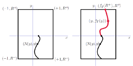
Figure 1: Simple vertical pipe configuration.

We now refer to the problem configuration in Figure 1. Given a positive constant $Q$, and functions $N:[R^{-},0]\to(-1,1)$ and $g:[-1,1]\to\mathbb{R}$, we want to find $u:(-1,1)\times(R^{-},R^{+})\to\mathbb{R}$ and free interface $\Gamma$ represented by

$$\Gamma=\{(y,f_{\Gamma}(y));\mbox{ with }0\leq y\leq R^{+}\}$$

where $f_{\Gamma}:[0,R^{+}]\to\mathbb{R}$ is such that $f_{\Gamma}(0)=N(0)$ (see Figure 1 right picture). The function $u$ and the free interface $\Gamma$ satisfy

$$\Delta u=0\mbox{ in }\Omega^{-}\quad\mbox{ and }\quad\Delta u=0\mbox{ in }\Omega^{+}$$ (21)

where

$$\Omega^{+}=\{-1<x<N(y),~{}R^{-}<y\leq 0\}\cup\{-1<x<f_{\Gamma}(y),~{}0\leq y<R^{-}\}$$

$$\Omega^{-}=\{N(y)<x<1,~{}R^{-}<y\leq 0\}\cup\{f_{\Gamma}(y)<x<1,~{}0\leq y<R^{-}\}.$$

The function $u$ has to satisfy the following known given data,

$$u(N(y),y)=0,\quad R^{-}<y<0;$$ (22)

$$u(x,R^{-})=g(x),\quad-1<x<1;$$ (23)

$$\frac{\partial u}{\partial y}u(x,R^{+})=0,\quad-1<x<1;$$ (24)

$$u(-1,y)=Q,\quad R^{-}<y<R^{+};$$ (25)

$$u(1,y)=-1,\quad R^{-}<y<R^{+};$$ (26)

and the following conditions on the free interface

$$u=0, \mbox{ on }\Gamma\quad(\mbox{ or }u(f_{\Gamma}(y),y)=0,0\leq y<R^{+}\mbox{)}$$ (27)

$$(\partial_{\eta}u^{+})^{2}-(\partial_{\eta}u^{-})^{2}=\lambda \mbox{ on }\Gamma$$ (28)

where $\lambda$ is given by

$$\lambda=\left(\frac{1}{1+b}\right)^{2}-\left(\frac{Q}{2-b}\right)^{2}.$$ (29)

We note that the boundary condition on the top of the domain (see Figure 1) is the homogeneous Neumann boundary condition, hence, the free boundary is not fixed at the top. That is, the value $f_{\Gamma}(R+)$ is not prescribed.

For each value of $b\in(-1,1)$, we can compute $\lambda$ through (29) and use our method to find an approximation of $u=u^{b}$ and $\Gamma=\Gamma^{b}$ (represented by $f_{\Gamma}=f_{\Gamma}^{b}$) that solve (21)-(29). Since the free boundary must have the vertical line $x=b$ as an asymptote, a feasible approximation of the free interface $\Gamma$ is obtained if $b=b^{*}$ where

$$b^{*}=f_{\Gamma}^{b^{*}}(R^{+}).$$ (30)

This is compatible with the asymptote condition $\lim_{y\to\infty}f_{\Gamma}(y)=b^{*}$.

Next, we use a bisection algorithm (applied to the function $(-1,1)\ni b\mapsto f_{\Gamma}^{b}(R^{+})\in(-1,1)$) to find the correct value of $b^{*}$ such that (30) is satisfied.

In the two examples presented next we run our method described in Subsection 3.1 until $\|\sigma^{h}_{n}\|_{L^{\infty}}<tol=10^{-6}$.

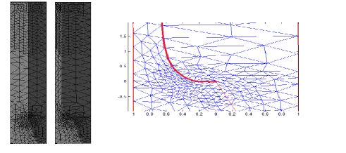
Figure 2: Free interface that solves (21)-(29) and (30) with $N(y)=0.5|y|/R^{-}$, $g(x)=(x-0.5)/1.5$ if $-1<x<0.5$, $g(x)=5(x-0.5)/0.5$ if $0.5<x<1$, $Q=5$ and $b^{*}=1/3$. Initial configuration (Left), final configuration (Middle) and a zoom around $(0,0)$ showing the free interface and the final mesh (Right).

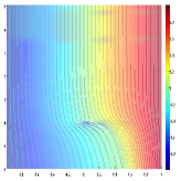
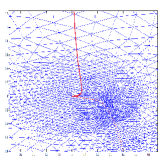
Figure 3: Function $u$ and free interface $\Gamma$ that solve (21)-(29) and (30) with $N(y)=0.5(|y|/R^{-})^{0.25}$, $g(x)=(x-0.5)/1.5$ if $-1<x<0.5$ , $g(x)=(x-0.5)/0.5$ if $0.5<x<1$, $Q=1$ and $b^{*}=1$. Solution (Left) and zoom around $(0,0)$ showing the free interface and the final mesh (Right)

The first example considers the nozzle represented by $N(y)=0.5|y|/R^{-}$ with $Q=5$. The data on the bottom is given by, $h(x)=(x-0.5)/1.5$ if $-1<x<0.5$ and $h(x)=5(x-0.5)/0.5$ if $0.5<x<1$. We obtain $b^{*}=1/3$. The initial free boundary approximation $\Gamma_{0}$ is the strait line from $(0,0)$ to $(0,R^{+})$ The resulting free boundary is displayed in Figure 2.

In the second example of jet flow problem we consider the nozzle represented by $N(y)=0.5(|y|/R^{-})^{0.25}$ with $Q=1$ and the Dirichlet data on the bottom side given by $h(x)=(x-0.5)/1.5$ if $-1<x<0.5$ and $h(x)=(x-0.5)/0.5$ if $0.5<x<1$. We obtained $b*=1$. The initial free boundary approximation $\Gamma_{0}$ is the strait line from $(0,0)$ to $(0,R^{+})$. The resulting free boundary and numerical solution (with constant lines -stream lines) are displayed in Figure 3.

5 Application to a free boundary problem arising in magnetohydrodynamics

In this section we apply our methodology to the model of plasma problem studied in [10, 12]. Here we are interesting in modeling the plasma confined in a Tokamac machine. More specifically, given $\Omega\subset\mathbb{R}^{2}$ and the positive constants $\gamma$ and $\lambda$, the plasma problem is to find $u$, a closed curve $\Gamma$ lying in $\Omega$ and a positive constant $\beta$ such that

$$\left\{\begin{array}[]{rll}-\Delta u=\beta u&&\mbox{ in }\Omega^{-}=\mbox{int}\{x\in\Omega,u(x)\leq 0\},\\ \int_{\Omega^{-}}u^{2}=1&&\\ -\Delta u=0&&\mbox{ in }\Omega^{+}=\{x\in\Omega,u(x)>0\},\\ u=\gamma&&\mbox{ on }\partial\Omega,\\ u=0&&\mbox{ on }\Gamma\mbox{ and }\Gamma=\partial\Omega^{-},\\ |\partial_{\eta}u^{+}|^{2}-|\partial_{\eta}u^{-}|^{2}=\lambda&&\mbox{ on}~{}\Gamma.\end{array}\right.$$ (31)

Here the plasma is enclosed by the curve $\Gamma$, and the complement of this region with respect to $\Omega$ is vacuum. The function $u$ represents a flux function associated to the magnetic induction $\vec{B}$, satisfying $\vec{B}=(u_{x_{2}},-u_{x_{1}},0)$.

It is easy to modify our method and apply it to this problem. We follow the description in Subsection 3.1 and iterate until $\|\sigma^{h}_{n}\|_{L^{\infty}}<tol=10^{-6}$. In this problem, the free boundary is a closed curve separating the domain in two connected components; as showed in [10]. The adaptation of our scheme to treat this problem is straightforward. We also mention that other formulations of the model, having the nonlinear condition on the free boundary, are also possible; see [10] and references therein.

In the first example, we consider the case of $\Omega$ being the ball with center $(0,0)$ and radius 1. We choose $\gamma=1$ and $\lambda=2^{2}-1^{2}=3$. The initial approximation of the free boundary is an ellipse centered at $(1/5,1/5)$ and with axis $1/3$ and $1/2$. The resulting configuration is depicted in Figure 4 and $\beta=13.6727$. We observe that the final shape of the free boundary approximates a circular region. This coincide with the results in [12] where the authors proved that for the domain $\Omega$ being the unit circle, the resulting free boundary is circular and centered at $(0,0)$. We note that in this example, the initial approximation of the free interface is far-off from the solution and despite of this fact, our algorithm still converges to the solution.

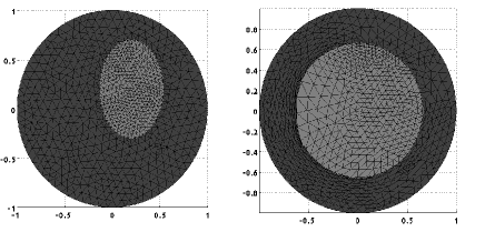
Figure 4: Free interface that solves (31) with $\Omega=\{(x,y):x^{2}+y^{2}<1\}$ , $\gamma=1$ and $\lambda=2^{2}-1^{2}=3$. Initial configuration: an ellipse centered at $(1/5,1/5)$ and with axis $1/3$ and $1/2$. (left). Final configuration (right).

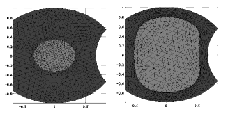
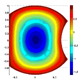
Figure 5: Free interface that solves (31) with depicted domain $\Omega$, $\gamma=1$ and $\lambda=5^{2}-1^{2}=4$. Initial configuration: the circle with center $(0,0)$ and radius $1/3$ (Left). Final configuration (Center). Solution (Right)

The second example considers the configuration described in Figure 5. The domain $\Omega$ corresponds to a circle from which it have been cut-off the region $\{y<-2/3\}$ and the intersection with the circle with center $(5/3,0)$ and radius 1. In this example we use $\lambda=5^{2}-1^{2}=4$. The initial approximation of the free boundary is a ball with center $(0,0)$ and radius $1/3$. The resulting free boundary is presented in Figure 5 (center) and the solution is plotted in Figure 5 (right). The computed value of $\beta=13.7034$.

6 Additional numerical examples

In this section we present some representative numerical examples. We run our method described in Subsection 3.1 until $\|\sigma^{h}_{n}\|_{L^{\infty}}<tol=10^{-6}$.

6.1 A known free interface and error decay

We consider problem (6) with $a_{1}=a_{2}=1$ and a known exact solution, what allows us to measure the accuracy of our method. The domain is $\Omega=[0,1]\times[0,1]$, $\lambda=-1$, the boundary data is given by $g(x,y)=2\min\{x-0.5,0\}+\max\{x-0.5,0\}$. We note that $u(x,y)=2\min\{x-0.5,0\}+\max\{x-0.5,0\}$ is a solution of the problem. For this exact solution, the free interface is the strait vertical line from $(0.5,0)$ to $(0.5,1)$.

We apply our method with the initial approximation of the free boundary given by $\Gamma_{0}=\{(x,y);y=0.5+0.1\sin(2\pi y)\}$ and the parameter $\tau=10^{-4}$. We present the initial and final subdomain configuration in Figure 6. In Figure 7 we present the $L^{\infty}$ norm of $\log(|\sigma^{h}|)$ in (14) along the number of iterations $n$. We observe a decay of the value $|\sigma^{h}|$ faster than $O(e^{-0.004n})$. This example also show that our stopping criteria is effective in the sense that at the last iteration, we see that the $L^{\infty}$ norm is already in stagnated plateau for the corresponding mesh size.

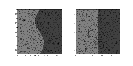
Figure 6: Results for the test problem in Section 6.1 Initial configuration (left). Final configuration (right).

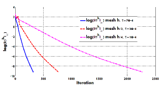
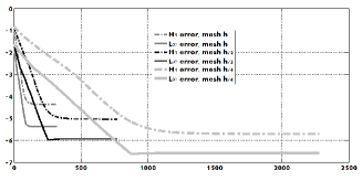
Figure 7: Result for the test problem in Section 6.1. We plot $\log(\|\sigma^{h}\|_{\infty})$ over the iterations requires to achieve $\|\sigma^{h}\|_{\infty}<10^{-4}$ for three different meshes (left). Corresponding solution error (in log scale) in $|\cdot|_{H^{1}(D)}$ and $L^{\infty}(D)$ norms.

6.2 An example with heterogeneous coefficients

This example considers a problem of type (6) with heterogeneous coefficient in each side of the free interface. We consider $\Omega=\{(x,y):x^{2}+y^{2}<1\}$ and the coefficient(s)

$$a_{1}(x,y)=\left\{\begin{array}[]{cc}100,&y\geq 0\\ 1,&y<0\end{array}\right.\quad\mbox{ and }\quad a_{2}(x,y)=\left\{\begin{array}[]{cc}1,&y\geq 0\\ 100,&y<0.\end{array}\right.$$

The Dirichlet data around the circle is given by $g(x,y)=x$ and we use $\lambda=-1$. The initial approximation of the free boundary is the strait line $\Gamma_{0}=\{(0,y),0\leq y\leq 1\}$. We run our method with $\tau=10^{-5}$. We show the resulting free boundary in Figure 8.

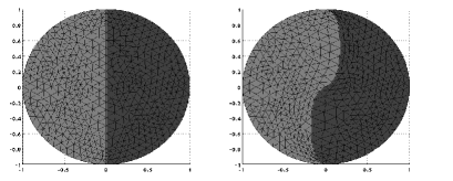
Figure 8: Results for the test problem in Section 6.2 that involves heterogeneous coefficients. Initial configuration (left). Final configuration (right)

7 Conclusions and comments

We have proposed a simple iterative method to handle free boundary problems involving nonlinear flux conditions. It is important to note, that the numerical treatment of nonlinear flux conditions on the free interface have not been extensively studied in the literature. This is the case despite of the fact that the mathematical analysis of simple models with nonlinear flux conditions on the free interface have been carried out by Caffarelli and coauthors a couple of decades ago. The proposed method is a simple domain decomposition method with inexpensive iterations. As a consequence it can be used for the better understanding of simplified models of complex flow problems. We present numerical results showing that, our iterative method is effective and perform well in several applications where nonlinear flux jump constrain drive the free interface behavior.

We obtained encouraging numerical results with our method but, its mathematical analysis is still needed. In a future work we plan to address mathematically questions related to the converge of the method. Other interesting numerical aspects we want to address are related to the implementation of adaptive refinement, the use of inexact local solvers (instead of exact subdomain solvers), and the design of preconditioners for our scheme. The extension to three dimensions can be considered.

We note that we consider simplified models of complicated flow problems. If we want to extend our method for more realistic models we need to consider time dependent problems. In this case, it would be important to be able to handle topological changes in the evolution of the free boundary.

Acknoledgements

The authors are thankful to Prof. Eduardo Teixeira for bringing this problem to our attention. H.M.V. was partially supported by FAPERJ grants E-26/102.965/2011, E-26/111.416 /2010. J.G. research is based in part on work supported by Award No. KUS-C1-016-04, made by King Abdullah University of Science and Technology (KAUST).

Appendix A An approximation of the flux

Given a free interface approximation $\Gamma^{h}$, we consider the approximation of the flux of $u^{h}$ (the solution of problem (12)) on ${\Omega^{+}_{h}}$.

Denote by $A=[a_{ij}]$ the Neumann finite element matrix defined by

$$a_{ij}=\int_{\Omega^{+}_{h}}a_{1}\nabla\phi_{i}\nabla\phi_{j}\;dx$$

where $\{\phi_{i}\}$ are the usual hat basis function of the space ${\cal P}^{1}(\mathcal{T}^{h}_{n},\Omega^{+}_{h})$.

We classify the nodes in interior nodes I, boundary nodes $\Sigma^{+}$ and interface notes $\Gamma$. This classification gives the following block structure of the matrix $A$,

$$A=\left(\begin{array}[]{ccc}A_{II}&A_{I\Sigma^{+}}&A_{I\Gamma}\\ A_{I\Sigma^{+}}^{T}&A_{\Sigma^{+}\Sigma^{+}}&A_{\Sigma^{+}\Gamma}\\ A_{I\Gamma}^{T}&A_{\Sigma^{+}\Gamma}^{T}&A_{\Gamma\Gamma}\\ \end{array}\right).$$

The solution of (12) is given by,

$$u^{h}=\left(\begin{array}[]{c}u_{I}^{h}\\ u_{\Sigma^{+}}^{h}\\ u_{\Gamma}^{h}\\ \end{array}\right)=\left(\begin{array}[]{c}A_{II}^{-1}(A_{I\Sigma^{+}}g^{h})\\ g^{h}\\ 0\\ \end{array}\right).$$

We define $\mu$ by

$$\mu=A_{I\Gamma}^{T}u_{I}=A_{I\Gamma}^{T}A_{II}^{-1}A_{I\Sigma^{+}}g^{h}.$$

Let $N_{\Gamma}$ be the number of vertices of $\cal{T}^{h}$ on $\Gamma^{h}$. We note that, using basic finite element analysis, we see that $\mu=(\mu_{i})\in\mathbb{R}^{N_{\Gamma}}$ with

$$\mu_{i}=\int_{\Omega^{+}_{h}}(a_{1}\nabla u^{h})\cdot\nabla\phi_{\ell_{i}}\;dx=\int_{\Gamma^{h}}(a_{1}\nabla u^{h})\cdot\eta_{\Gamma^{h}}\phi_{\ell_{i}}\;ds.$$

Here given $i\in\{1,...N_{\Gamma}\}$, $\ell_{i}$ represents the index of the a node of $\mathcal{T}^{h}$ belonging to $\Gamma^{h}$.

We use $\mu$ to obtain a piecewise linear approximation of the flux $\nabla u^{h}\cdot\eta_{\Gamma^{h}}$. Since $u^{h}=0$ on $\Gamma^{h}$, for each edge of $e_{k}$ of $\Gamma^{h}$ we have

$$\nabla u^{h}|_{e_{k}}=\partial_{\eta_{k}}u\eta_{k}$$

where $\eta_{k}$ represents the normal vector to edge $e_{k}$ pointing in the outward direction of $\Omega^{+}_{h}$. Hence,

$$\mu_{i}=\int_{\Gamma^{h}}(\eta_{\Gamma^{h}}^{T}a_{1}\eta_{\Gamma^{h}})\partial_{\eta_{\Gamma^{h}}}u\phi_{\ell_{i}}\;ds.$$ (32)

We define $\lambda^{h}_{1}$ the piecewise linear approximation of $\partial_{\eta_{\Gamma^{h}}}u$ as follows. First, we observe that $\lambda^{h}_{1}\in span\{\phi_{\ell_{i}}|_{\Gamma^{h}}\}_{1\leq i\leq N_{\Gamma}}$. Next we introduce the matrix $Q=[q_{ij}]\in\mathbb{R}^{N_{\Gamma}\times N_{\Gamma}}$ with

$$q_{ij}=\int_{\Gamma^{h}}(\eta_{\Gamma^{h}}^{T}a_{1}\eta_{\Gamma^{h}})\phi_{\ell_{i}}\phi_{\ell_{j}}\;ds.$$

Finally, based on relation (32) we define

$$\lambda^{h}_{1}=\sum_{i}^{N_{\Gamma}}\alpha_{i}\phi_{\ell_{i}}|_{\Gamma^{h}}$$ (33)

where $\alpha=(\alpha_{i})$ is the solution of

$$Q\alpha=\mu.$$

In a similar way we define $\lambda_{2}^{h}$, the approximation of of the flux on $\Gamma^{h}$, of the solution of (13).

Remark 3

A more regular approximation of the flux can be done in practice. For instance, we could obtain $\alpha$ as the solution of the following problem

$$(Q+\epsilon D)\alpha=\mu.$$

where $D$ is diffusion of operator on $\Gamma^{h}$ and $\epsilon$ is a regularization parameter.

References

- [1] Hans Wilhelm Alt, Luis A. Caffarelli, and Avner Friedman. Jets with two fluids. i. one free boundary. Indiana Univ. Math. J., 33(2):213–247, 1984.
- [2] Hans Wilhelm Alt, Luis A. Caffarelli, and Avner Friedman. Abrupt and smooth separation of free boundaries in flow problems. Ann. Scuola Norm. Sup. Pisa Cl. Sci. (4), 12(1):137–172, 1985.
- [3] John W. Barrett and Charles M. Elliott. Fixed mesh finite element approximations to a free boundary problem for an elliptic equation with an oblique derivative boundary condition. Comput. Math. Appl., 11(4):335–345, 1985.
- [4] F. Bouchon, S. Clain, and R. Touzani. Numerical solution of the free boundary Bernoulli problem using a level set formulation. Comput. Methods Appl. Mech. Engrg., 194(36-38):3934–3948, 2005.
- [5] S. Chen, B. Merriman, S. Osher, and P. Smereka. A simple level set method for solving Stefan problems. J. Comput. Phys., 135(1):8–29, 1997.
- [6] Zhiming Chen, Tsimin Shih, and Xingye Yue. Numerical methods for Stefan problems with prescribed convection and nonlinear flux. IMA J. Numer. Anal., 20(1):81–98, 2000.
- [7] Karsten Eppler and Helmut Harbrecht. Efficient treatment of stationary free boundary problems. Appl. Numer. Math., 56(10-11):1326–1339, 2006.
- [8] M. Flucher and M. Rumpf. Bernoulli’s free-boundary problem, qualitative theory and numerical approximation. J. Reine Angew. Math., 486:165–204, 1997.
- [9] Avner Friedman. The Stefan problem in several space variables. Trans. Amer. Math. Soc., 133:51–87, 1968.
- [10] Avner Friedman and Yong Liu. A free boundary problem arising in magnetohydrodynamic system. Ann. Scuola Norm. Sup. Pisa Cl. Sci. (4), 22(3):375–448, 1995.
- [11] S. L. Kamenomostskaja. On Stefan’s problem. Mat. Sb. (N.S.), 53 (95):489–514, 1961.
- [12] Kyung-Keun Kang, June-Yub Lee, and Jin Keun Seo. Identification of a free boundary arising in a magnetohydrodynamics system. Inverse Problems, 13(5):1301–1309, 1997.
- [13] Kari T. Kärkkäinen and Timo Tiihonen. Free surfaces: shape sensitivity analysis and numerical methods. Internat. J. Numer. Methods Engrg., 44(8):1079–1098, 1999.
- [14] Christopher M. Kuster, Pierre A. Gremaud, and Rachid Touzani. Fast numerical methods for Bernoulli free boundary problems. SIAM J. Sci. Comput., 29(2):622–634, 2007.
- [15] R. H. Nochetto, M. Paolini, and C. Verdi. An adaptive finite element method for two-phase Stefan problems in two space dimensions. I. Stability and error estimates. Math. Comp., 57(195):73–108, S1–S11, 1991.
- [16] R. H. Nochetto, M. Paolini, and C. Verdi. An adaptive finite element method for two-phase Stefan problems in two space dimensions. II. Implementation and numerical experiments. SIAM J. Sci. Statist. Comput., 12(5):1207–1244, 1991.
- [17] Eduardo V. Teixeira Raimundo Leitão, Olivaine S. de Queiroz. Regularity for degenerate two-phase free boundary problems. eprint arXiv:1202.5264, 2012.
- [18] L. I. Rubenstein. The Stefan problem. American Mathematical Society, Providence, R.I., 1971. Translated from the Russian by A. D. Solomon, Translations of Mathematical Monographs, Vol. 27.
- [19] Patricia Saavedra and L. Ridgway Scott. Variational formulation of a model free-boundary problem. Math. Comp., 57(196):451–475, 1991.
- [20] K. G. van der Zee, E. H. van Brummelen, and R. de Borst. Goal-oriented error estimation and adaptivity for free-boundary problems: the domain-map linearization approach. SIAM J. Sci. Comput., 32(2):1064–1092, 2010.
- [21] Augusto Visintin. Introduction to Stefan-type problems. In Handbook of differential equations: evolutionary equations. Vol. IV, Handb. Differ. Equ., pages 377–484. Elsevier/North-Holland, Amsterdam, 2008.
- [22] Zhimin Zhang and Ivo Babuška. A numerical method for steady state free boundary problems. SIAM J. Numer. Anal., 33(6):2184–2214, 1996.