Capture numbers and island size distributions
in models of submonolayer surface growth

Abstract

The capture numbers entering the rate equations (RE) for submonolayer film growth are determined from extensive kinetic Monte Carlo (KMC) simulations for simple representative growth models yielding point, compact, and fractal island morphologies. The full dependence of the capture numbers $\sigma_{s}(\Theta,\Gamma)$ on island size $s$, and on both the coverage $\Theta$ and the $\Gamma=D/F$ ratio between the adatom diffusion coefficient $D$ and deposition rate $F$ is determined. Based on this information, the RE are solved to give the RE island size distribution (RE-ISD), as quantified by the number $n_{s}(\Theta,\Gamma)$ of islands of size $s$ per unit area. The RE-ISDs are shown to agree well with the corresponding KMC-ISDs for all island morphologies. For compact morphologies, however, this agreement is only present for coverages smaller than $\Theta\simeq 5\%$ due to a significantly increased coalescence rate compared to fractal morphologies. As found earlier, the scaled KMC-ISDs $n_{s}\bar{s}^{2}/\Theta$ as a function of scaled island size $x=s/\bar{s}$ approach, for fixed $\Theta$, a limiting curve $f_{\infty}(x,\Theta)$ for $\Gamma\to\infty$. Our findings provide evidence that the limiting curve is independent of $\Theta$ for point islands, while the results for compact and fractal island morphologies indicate a dependence on $\Theta$.

I Introduction

The kinetics of submonolayer nucleation and island growth during the initial stage of epitaxial thin film growth has been studied intensively both experimentally and theoretically for more than three decades (for reviews, see Refs. Brune, 1998; Michely and Krug, 2004; Evans et al., 2006; Dieterich et al., 2008a, and references therein). Important aspects of the growth kinetics in the submonolayer growth regime can be described by the rate equations (RE) approach.Venables (1973) This approach has proven to be very valuable in inorganic thin film growth. Interestingly, many of the theoretical concepts developed for thin film growth kinetics of inorganic materials, have shown recently to be very valuable also for applications in organic thin film growth.Hlawacek et al. (2008); Loske et al. (2010); Zangwill and Vvedensky (2011); Potocar et al. (2011); Körner et al. (2011) This is due to the fact that these concepts often are not specifically referring to particular materials. Instead, they take into account the key mechanisms involved in the complex interplay of deposition, evaporation, diffusion, aggregation and dissociation from a general viewpoint.

Parameters entering the RE are the capture numbers $\sigma_{s}(\Theta,\Gamma)$, which describe the strength of islands of size $s$ to capture adatoms at a coverage $\Theta$ and ratio $D/F\equiv\Gamma$ of the adatom diffusion coefficient $D$ and deposition flux $F$. The dependence of the capture numbers on $s$ has been studied for various $\Gamma$ but only for one or a few $\Theta$ values. In this work we present a systematic study of the full dependence on both $\Theta$ and $\Gamma$ for different types of island morphologies and the case, where detachments of atoms from islands can be neglected, corresponding to a critical nucleus of size $i=1$. This is motivated by the following questions, which have not been thoroughly answered yet:

• If the $\sigma_{s}(\Theta,\Gamma)$ are known, do the RE then predict correctly the number density $n_{s}(\Theta,\Gamma)$ of islands of size $s$, that means the island size distribution (ISD)? This question indeed was earlier posed by Ratsch and Venables Ratsch and Venables (2003) as well as Evans et al. Evans et al. (2006) The answer to this question is not obvious, since the RE with known capture numbers $\sigma_{s}(\Theta,\Gamma)$ neglect many-particle correlation effects,com spatial fluctuations in shapes and capture zones of islands, and coalescence events that, despite rare in the early-stage growth, can have a significant influence.Körner et al. (2010)

• Is there a simple functional form of the $\sigma_{s}(\Theta,\Gamma)$, in particular, is there a scaling of these capture numbers with respect to an effective capture length as suggested by a self-consistent treatment Bales and Chrzan (1994); Bales and Zangwill (1997) based on the RE? Do the $\sigma_{s}$, when scaled with respect to their mean $\bar{\sigma}$, depend for large $\Gamma$ on the scaled island size $s/\bar{s}$ only, as suggested by Bartelt and Evans Bartelt and Evans (1996)?

In previous studies it has been found that the scaled ISD $\bar{s}^{2}n_{s}/\Theta$ as a function of scaled island size $x=s/\bar{s}$ approaches, for fixed coverage $\Theta$, a scaling function $f(x)$ for large $\Gamma$. Early simulations suggested that $f(x)$ is independent of $\Theta$ and moreover not sensitive to the island morphology. However, later results showed Bartelt and Evans (1996); Evans et al. (2006) that the morphology has an influence on the form of $f(x)$. In fact, one would expect the scaling function $f(x)$ to become independent of $\Theta$ if the RE with known capture numbers correctly predict the ISD, and if the scaled capture numbers $\sigma/\bar{\sigma}$ as a function of $s/\bar{s}$ become independent of $\Theta$ for large $\Gamma$. Under these assumptions, an explicit relation was proposed by Bartelt and Evans,Bartelt and Evans (1996); Evans and Bartelt (2001) which connects the scaling function of the capture numbers with the scaling function of the ISD. We hence address the following further questions:

• Is the scaling function $f(x)$ independent of $\Theta$ for large $\Gamma$? What is the influence of the island morphology? Can the relation between the scaled ISD $f(x)$ and the scaling function for the capture numbers be confirmed?

The RE treatment is based on a coupled set of simple rate equations describing the time evolution of the adatom density $n_{1}$ and the number density $n_{s}$ of islands with size $s\geq 2$, if spatial correlations among islands during growth are neglected. Taking into account direct impingement of arriving atoms at the border of islands, the RE for the case $i=1$ read

$$\frac{1}{F}\frac{\mathrm{d}n_{1}}{\mathrm{d}t}= (1-\Theta)-2\Gamma\sigma_{1}n_{1}^{2}-\Gamma n_{1}\sum_{s>1}\sigma_{s}n_{s}$$

$${}-2\kappa_{1}n_{1}-\sum_{s>1}\kappa_{s}n_{s}\,$$ (1)

$$\frac{1}{F}\frac{\mathrm{d}n_{s}}{\mathrm{d}t}= \Gamma n_{1}\left(\sigma_{s-1}n_{s-1}-\sigma_{s}n_{s}\right)$$

$${}+\kappa_{s-1}n_{s-1}-\kappa_{s}n_{s}\,,\quad s=2,3,\ldots$$ (2)

These equations refer to the pre-coalescence regime where only adatoms are mobile and it is presumed that re-evaporation of atoms and atom movements between the first and second layer can be disregarded. Moreover, adatoms arriving on top of an island are not counted, i.e. $s$ in a strict sense refers to the number of substrate sites covered by an island (or the island area). The coverage $\Theta$ entering Eq. (I) is given by $\Theta=\sum_{s\geq 1}sn_{s}=1-\exp(-Ft)$ and takes into account that adatoms are generated by deposition into the uncovered substrate area (as common in the literature in this field, we set the length unit equal to the the size of the substrate lattice unit). The terms with $\sigma_{1}(\Theta)$ and $\kappa_{1}(\Theta)$ describe the nucleation of dimers due to attachment of two adatoms by diffusion and due to direct impingement, respectively. The term $\propto n_{1}\sigma_{s}n_{s}$ describes the attachment of adatoms to islands of size $s>1$, and the term $\propto\kappa_{s}n_{s}$ the direct impingement of deposited atoms to boundaries of islands with size $s$. For the idealized point island model, $s$ refers to the total number of atoms that arrived at a point, and $(1-\Theta)$ in Eq. (I) is replaced by one (no covered substrate area). For a unified discussion of capture numbers and the ISD we formally set $\Theta=Ft$ for the point island model.

Introducing the total number density of stable islands $N$ and the average capture number $\overline{\sigma}$,

$$N =\sum\limits_{s>1}n_{s},\quad\overline{\sigma}=\frac{1}{N}\sum_{s>1}\sigma_{s}n_{s}\,,$$ (3)

a reduced set of equations for $n_{1}(\Theta)$ and $N(\Theta)$ can be derived from Eqs. (I) and (2) within the RE treatment. These equations predict the scaling relation $N\propto\Gamma^{-\chi}$ with the scaling exponent $\chi=1/3$.Venables et al. (1984); Venables (1994) This relation has been successfully validated by several growth experiments in the past and applied to extract adatom diffusion barriers and binding energies in metal epitaxy. A discussion of many of these experiments can be found in Ref. Michely and Krug, 2004. Recently, the relation has also been applied in organic thin film growth .Loske et al. (2010); Hlawacek et al. (2008) An extended RE approach for multicomponent adsorbates Einax et al. (2007); Dieterich et al. (2008a) was recently suggested to determine binding energies between unlike atoms from island density data.Einax et al. (2009)

More detailed information on the growth kinetics is contained in the ISD. If the full dependence of the ISD $n_{s}(\Theta,\Gamma)$ on $\Theta$ and $\Gamma$ is mediated by the mean island size $\bar{s}(\Theta,\Gamma)$, the ISD should obey the following scaling form, as first suggested by Vicsek and Family,Vicsek and Family (1984)

$$\frac{{\overline{s}}^{2}(\Theta,\Gamma)}{\Theta}n_{s}(\Theta,\Gamma)=f\left(\frac{s}{\bar{s}(\Theta,\Gamma)}\right)\;\;.$$ (4)

Here the scaling function $f(x)$ must fulfill the conditions $\int_{0}^{\infty}f(x)dx=\int_{0}^{\infty}xf(x)dx=1$. The scaling behavior was found to give a good effective description for large $\Gamma$. More precisely, the curves ${\overline{s}}^{2}n_{s}/\Theta$ as a function of $x=s/\bar{s}$ approach a limiting curve, Vvedensky (2000)

$$\lim_{\Gamma\to\infty}\frac{{\bar{s}}^{2}}{\Theta}n_{x\bar{s}}(\Theta,\Gamma)=f_{\infty}(x,\Theta)\,.$$ (5)

Previous studies for a few fixed $\Theta$ values suggest that $f_{\infty}(x,\Theta)$ is independent of $\Theta$.

An explicit expression for the scaling function $f(x)$ with shape independent of $\Theta$ was suggested by Amar and Family,Amar and Family (1995)

$$f(x)=C_{i}x^{i}\exp\left(-ia_{i}x^{1/a_{i}}\right)\,.$$ (6)

The parameters entering this scaling function depend on the size of the critical nucleus $i$, which allows one to determine $i$ in experiments.Loske et al. (2010); Potocar et al. (2011); Ruiz et al. (2003); Pomeroy and Brock (2006) Equation (6) was believed to be independent even of the morphology Amar and Family (1995), but this has later been questioned.Bartelt and Evans (1996); Evans et al. (2006)

Based on a continuum limit of the RE (2) and scaling assumptions for the capture numbers and a neglect of the $\Theta$-dependence, an expression for the limiting curve $f_{\infty}(x)$ was derived by Bartelt and Evans, Bartelt and Evans (1996); Evans and Bartelt (2001)

$$f_{\infty}(x)=f_{\infty}(0)\exp\left\{\int_{0}^{x}{\rm d}y\frac{(2z_{\infty}-1)-C_{\rm tot}^{\prime}(y)}{C_{\rm tot}(y)-zy}\right\}\,,$$ (7)

where $z_{\infty}={\mathrm{\partial}(\ln\bar{s})/\mathrm{\partial}(\ln\Theta)}$, and $C_{\rm tot}(x)$ is a linear combination of the scaled capture numbers $C_{\infty}(x)=\sigma_{s}/\bar{\sigma}$ and scaled direct capture areas $K_{\infty}(x)=\kappa_{s}/\bar{\kappa}$. The $\infty$-subscript indicates that the large $\Gamma\to\infty$ limit should be taken. As pointed out by Bartelt and Evans, $C_{\rm tot}(x)$ should be well approximated by the scaled capture numbers alone, $C_{\rm tot}(x)\approx(1-\Theta)C_{\infty}(x)$. In Appendix A we show that in fact it holds $C_{\rm tot}(x)\approx C_{\infty}(x)$. The two conditions for $f_{\infty}(x)$ (normalization and first moment equal to one) imply that $C_{\infty}(0)=(1-z)/f_{\infty}(0)$ and $\int_{0}^{\infty}dx\,C_{\infty}(x)f_{\infty}(x)=1$. Evans and Bartelt (2001); Evans et al. (2006)

It is interesting to note that a semi-empirical form, which has a structure similar to Eq. (6) has been suggested recently by Pimpinelli and Einstein Pimpinelli and Einstein (2007) for the distribution of capture zones $A$ as identified by Voronoi tessellation,

$$P_{\beta} =c_{\beta}a^{\beta}\exp(-d_{\beta}a^{2})\,,$$ (8)

where $a=A/\bar{A}$ is the rescaled capture zone with respect to the mean $\bar{A}$ and $\beta=i+1$ (see also Ref. Oliveira and Aarão Reis, 2011). This distribution corresponds to a generalized Wigner surmise from random matrix theory. The parameter $\beta=i+1$ and the functional form, however, are controversially discussed.Li et al. (2010); Pimpinelli and Einstein (2010)

Besides this recent progress in predicting functional forms of capture zone distributions, there are only a few studies so far Gibou et al. (2001, 2003); Körner et al. (2010) that address the problem whether an integration of the RE (I) and (2) can yield correctly the ISD for different cluster morphologies in the pre-coalescence regime. For an integration of the RE a reliable determination of $\sigma_{s}(\Theta,\Gamma)$ is needed. Four general approaches have been followed for this purpose: (i) Within a self-consistent ansatz one can solve the diffusion field around an island and derive determining equations for the capture numbers by equating the attachment currents of the diffusion field and the RE. Bales and Chrzan (1994); Bales and Zangwill (1997) (ii) By modeling the island growth with the level set method, Gyure et al. (1998) one can analogously equate attachments currents and determine the capture numbers.Gibou et al. (2001, 2003) (iii) Balancing the deposition rate $FA_{s}n_{s}$ into the mean capture zone $A_{s}$ of islands of size $s$ with the RE expression $D\sigma_{s}n_{1}n_{s}$ for the attachment rate to these islands, yields $\sigma_{s}\simeq A_{s}/\Gamma n_{1}$. This means that the capture numbers can be approximately calculated from a determination of the $A_{s}$, e.g. by Voronoi tessellation.Bartelt et al. (1999a); Evans and Bartelt (2001); Bartelt et al. (1998); Hannon et al. (1998) (iv) In simulations, where the individual attachments are followed, the capture numbers can be calculated from the mean number of attachments $M_{s}$ to island of size $s$ during a time interval $\Delta t$ [see Eq. (9) and the discussion in Sec. II].Bartelt and Evans (1996)

The paper is organized as follows. First we describe in Sec. II the method used to generate point, compact and fractal island morphologies, and the method for determining the capture numbers as function of island size and coverage. In Sec. III we discuss the results for the capture numbers and compare these with the prediction of the self-consistent theory. In Sec. IV we analyze the mean island and adatom densities for the different island morphologies and discuss their prediction by the self-consistent RE and the RE based on the capture numbers determined in the KMC simulations. In Sec. V we demonstrate that the ISD is successfully predicted by the RE as long as coalescence events can be neglected. These coalescence events are relevant already for small coverages $\Theta\gtrsim 0.05$ for compact morphologies, while they turn out to be much less important for fractal morphologies. The reason for these differences are reduced coalescence rates for fractal island morphologies because of a screening effect.Brune (1998); Brune et al. (1999) Finally, we study in Sec. VI the behavior of the scaled capture numbers and scaled ISDs in the limit $\Gamma\to\infty$.

II Submonolayer growth: models, morphologies and simulations

The KMC simulations are performed with a first reaction time Monte Carlo algorithm Holubec et al. (2011); Gillespie (1977) on a square lattice with $L\times L$ sites. In this algorithm, two times $\tau_{F}$ and $\tau_{D}$ are randomly generated from the exponential probability density $\psi(\tau)=\gamma\exp(-\gamma\tau)$, where $\gamma=L^{2}F$ for $\tau_{F}$, corresponding to a deposition process, and $\gamma=4DL^{2}n_{1}$ for $\tau_{D}$, corresponding to one of the possible diffusive jumps of adatoms. If $\tau_{D}<\tau_{F}$, the simulation time is incremented by $\tau_{D}$ and one of the $L^{2}n_{1}$ adatoms is selected randomly and moved to a randomly selected vacant nearest neighbor site. If $\tau_{F}<\tau_{D}$, the simulation time is incremented by $\tau_{F}$ and one of the $L^{2}$ sites is randomly chosen. If this site is vacant, an additional adatom is deposited on this site, while, if the site is occupied, no deposition takes place.

With respect to the formation of islands we consider three simple growth models that are representative for the different types of island morphologies in the case of $i=1$. Fractal islands are generated by applying “hit and stick” aggregation, that means an adatom having another atom as nearest neighbor becomes immobilized. Compact island morphologies are produced by letting islands grow spirally into a quadratic form as in Ref. Bartelt and Evans, 1993, meaning that each adatom attaching to an island is displaced to the corresponding tip of the spiral. Point island morphologies are generated by displacing an adatom attaching to an island to the site representing the island, while bookkeeping the total number of aggregated atoms for the island size.

Figure 1: Capture numbers as a function of $s$ for $\Gamma=10^{7}$ and four different fixed coverages for the models representing (a) point, (b) compact, and (c) fractal island morphologies. The filled symbols refer to the $\sigma_{s}$ obtained from the KMC simulations and the open symbols to the results of the self-consistent theory according to Eqs. (10) (with the $R_{s}$ taken from the simulations, see text and Fig. 3).

Figure 2: Mean capture number $\bar{\sigma}$ and mean island size $\bar{s}$ as a function of $\Theta$ for the four simulated $\Gamma$ values and the models representing point, compact and fractal island morphologies.

To calculate the capture numbers $\sigma_{s}$ at the coverage $\Theta$, we use the following procedure which is based on the method outlined in Ref. Bartelt and Evans, 1996: Each simulation run is stopped at coverage $\Theta$ and the number densities $n_{s}=N_{s}/L^{2}$, $s=1,2,\ldots$ are determined, where $N_{s}$ are the numbers of monomers ($s=1$) and islands ($s>1$). Then the simulation is continued for a time interval $\Delta t$ without deposition and the following additional rules are implemented: (i) if an adatom is attaching to an island of size $s>1$, a counter $M_{s}$ is incremented and the adatom thereafter repositioned at a randomly selected site on the free substrate area (i.e. a site which is neither covered nor a nearest neighbor of a covered site); (ii) if two adatoms form a dimer, a counter $M_{1}$ is incremented and the two adatoms thereafter are repositioned randomly as described in (i). In this way a stationary state is maintained at the coverage $\Theta$. The mean attachment rate per unit area to islands of size $s$ is $M_{s}/(L^{2}\Delta t)$, and equating this with the expression $D\sigma_{s}n_{s}n_{1}$ from the RE (I,2) yields

$$\sigma_{s}=\frac{M_{s}}{L^{2}\Delta tDn_{s}n_{1}} s=1,2,\ldots$$ (9)

Averaging over many simulation runs (configurations) gives $\sigma_{s}(\Theta,\Gamma)$. The $\kappa_{s}$ are determined from the lengths of the islands boundaries, which are simultaneously monitored during the simulation and averaged for each size $s$.

The continuous-time Monte Carlo (KMC) simulations are performed on a square lattice with periodic boundary conditions and $L\times L=8000\times 8000$ sites for four different $\Gamma=10^{5}$, $10^{6}$, $10^{7}$, and $10^{8}$. For each value of $\Theta$ an average over $10^{8}$ nucleation/attachment events was performed.

III Capture numbers

The direct capture areas for point islands on a square lattice are given by $\kappa_{s}=4$. For compact and fractal islands the $\kappa_{s}$ increase as $\sim\sqrt{s}$ and $\sim s$, respectively, and their dependence on $\Theta$ and $\Gamma$ is very weak.

Representative results for the capture numbers $\sigma_{s}$ are shown in Fig. 1 as a function of $s$ for fixed $\Gamma=10^{7}$ and four different coverages for the (a) point, (b) compact, and (c) fractal island morphologies. For the other simulated $\Gamma$ values, a similar behavior was obtained. The mean $\bar{\sigma}(\Theta,\Gamma)$ [see Eq. (3)] as a function of $\Theta$ for all simulated $\Gamma$ values is displayed in Fig. 2, together with the mean island size $\bar{s}(\Theta,\Gamma)$. These functions are later used in Sec. VI when investigating the scaled capture numbers $\sigma_{s}$ in connection with the scaled island densities in the limit $\Gamma\to\infty$.

A common feature for all morphologies in Fig. 1 is a linear increase of $\sigma_{s}$ with $s$ for large $s>\bar{s}$. It can be understood Evans et al. (2006) from the proportionality of the $\sigma_{s}$ to the mean capture zone areas $A_{s}$, and the fact that large islands typically exhibit large $A_{s}$, which led to the stronger growth of these islands. Since a twice as large capture zone gives on average rise to a twice as large island, it holds $A_{s}\sim s$ and hence $\sigma_{s}\propto A_{s}\sim s$. Bartelt and Evans (1996); Evans et al. (2006)

With respect to the dependence on the coverage $\Theta$, the $\sigma_{s}$ in Fig. 1 have a quite different behavior for the three morphologies in the regime $s>\bar{s}$: While for the point islands the $\sigma_{s}$ decrease with $\Theta$, they are almost independent of $\Theta$ for the compact islands, and they increase with $\Theta$ for the fractal islands. Main reason for these differences is that for point islands the number density $N$ continues to increase with $\Theta$ (that means time $t=\Theta/F$) due to ongoing nucleation of new islands, while for compact and fractal morphologies, $N$ tends to saturate for larger $\Theta$, with less pronounced saturation in the compact case (see Sec. IV below). During the growth in the point island model, a large capture zone surrounding a large island is, compared to the other two morphologies, more frequently destroyed by a nucleation event in this zone, and the $A_{s}\propto\sigma_{s}$ thus decrease with $\Theta$ for fixed $s>\bar{s}$. Due to the higher nucleation rate and the missing spatial extension of islands in the point island model, the corresponding $\sigma_{s}$ are much smaller than for the compact and fractal morphologies. The larger island extension and the strong capture of adatoms by finger tips in the case of fractal islands lead to about five times larger $\sigma_{s}$ in comparison to the compact islands.

The differences with respect to the $\Theta$ dependence are also reflected in the behavior of $\bar{\sigma}(\Theta,\Gamma)$ in Fig. 2. In fact, when considering the scaled capture numbers $\sigma_{s}/\bar{\sigma}$, the $\Theta$ dependence for $s>\bar{s}$ becomes qualitatively the same for all morphologies (increase of $\sigma_{s}/\bar{\sigma}$ with $\Theta$, see Sec. VI below). For small $s<\bar{s}$, the curves in Fig. 1 show a nonlinear dependence of $\sigma_{s}$ on $s$ for all morphologies.Bartelt et al. (1998, 1999b); Amar et al. (2001) By combining the linear function for large $s$ with a polynomial at small $s$, we fitted the results for $\sigma_{s}$ for all simulated $\Theta$ and $\Gamma$ values. These fits, together with corresponding fits for the $\kappa_{s}$, were used to integrate the RE (I) and (2).

The mean island size $\bar{s}$ in Fig. 2 reproduces the behavior seen in many earlier studies. Evans et al. (2006) In the point island model the straight lines in the double logarithmic representation are in agreement with $\bar{s}\sim\Theta^{z}$ with $z={2/3}$ as predicted by a scaling analysis of the reduced RE.Bartelt and Evans (1992); Evans et al. (2006); Dieterich et al. (2008b) In the case of the compact and fractal island morphologies, the slope $z(\Theta)=\partial\ln s(\Theta,\Gamma)/\partial\ln\Theta$ increases with $\Theta$ and approaches $z\simeq 1$ for both island morphologies. This is consistent with a saturation ($\Theta$-independence) of the island density for large $\Theta$ in the pre-coalescence regime, $\bar{s}\sim\Theta/N\sim\Theta$.

Figure 3: Mean radii of gyration $R_{s}$ of islands of size $s$ for the models representing compact and fractal island morphologies. The straight lines in the double-logarithmic plot indicate the power-law behavior for large $s$.

In the self-consistent theory Bales and Chrzan (1994) the capture numbers are given by

$$\sigma_{s}^{\rm sc} =\frac{2\pi}{(1-\Theta)}\frac{R_{s}}{\xi}\frac{{K}_{1}\left(R_{s}/\xi\right)}{{K}_{0}\left(R_{s}/\xi\right)}\,,$$ (10a)

$$\xi^{-2} =2\sigma_{1}^{\rm sc}n_{1}+\sum_{s\geq 2}\sigma_{s}^{\rm sc}n_{s}\,,$$ (10b)

where $R_{s}$ is the effective radius of an island of size $s$, $K_{0}$ and $K_{1}$ are the modified Bessel functions of order zero and one, respectively, and $\xi$ is the adatom capture length (mean linear size of depletion zone around an island). The factor $(1-\Theta)$ in Eq. (10), which was not given in the original derivation in Ref. Bales and Chrzan, 1994 arises from the fact that the adatom current to a (circular) island of size $s$ is $2\pi R_{s}D\,\partial_{r}\tilde{n}_{1}(r)|_{r=R_{s}}$, where $\tilde{n}_{1}(r)=n_{1}(r)/(1-\Theta)$ is the adatom density with respect to the free (uncovered) surface area, and $n_{1}(r)$ is the local form corresponding to the global mean value $n_{1}$ appearing in the RE [see also Ref. Popescu et al., 2001 for the additional factor $(1-\Theta)$]. For $R_{s}\ll\xi$, $\sigma_{s}\sim 2\pi/[(1-\Theta)\ln(\xi/R_{s})]$, and for $R_{s}\gg\xi$, $\sigma_{s}\sim 2\pi/(1-\Theta)(R_{s}/\xi)$.

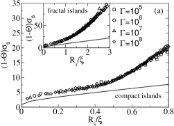
Figure 4: Scaling plot of $(1-\Theta)\sigma_{s}$ as a function of $R_{s}/\xi$ for the model representing compact island morphologies, with both $R_{s}$ and $\xi^{-2}=2\sigma_{1}n_{1}+\sum_{s\geq 2}\sigma_{s}n_{s}$ determined from the KMC simulations, (a) for various $\Gamma$ and fixed $\Theta=0.2$, and (b) for various $\Theta$ and fixed $\Gamma=10^{8}$. The insets in (a) and (b) show the corresponding results for the model representing fractal island morphologies. The solid lines represent the specific functional form in Eq. (10) predicted by the self-consistent theory.

Figure 5: KMC results (symbols) for the adatom density $n_{1}$ and island density $N$ as function of $\Theta$ at $\Gamma=10^{7}$ for (a) point, (b) compact, and (c) fractal island morphologies in comparison with the RE solutions, when using the direct capture areas $\kappa_{s}$ and capture numbers $\sigma_{s}$ from Sec. III (solid lines) and when using the capture numbers $\sigma^{\rm sc}_{s}$ from the self-consistent theory according to Eq. (10) (dashed lines).

To determine the $\sigma_{s}^{\rm sc}$, the RE (I) and (2) are numerically solved with initial conditions $n_{s}=0$ at time $t=0$ and a cutoff value $s_{c}$ so that $n_{s}$ can be safely neglected for $s>s_{c}$. In each integration step the implicit Eq. (10) is solved for the $\sigma_{s}^{\rm sc}$. The results become sensitive to the island morphology via the dependence of $R_{s}$ on $s$ in this approach. For point islands we take $R_{s}=1$ corresponding to one lattice constant. For the compact and fractal island morphologies, we determined the mean radius of gyration of islands of size $s$, as shown in Fig. 3. The straight lines in the double-logarithmic representation give $R_{s}\sim 0.42s^{1/2}$ (compact islands) and $R_{s}\sim 0.47s^{0.57}$ (fractal morphologies) for large $s$. To compare the $\sigma_{s}^{\rm sc}$ with the $\sigma_{s}$ obtained from the KMC simulations, we used the full dependence of the $R_{s}$ on $s$, i.e. including the small $s$ behavior, in our integration of the RE. The results from the self-consistent theory are shown in Fig. 1 (open symbols). As can be seen from the figure, the $\sigma_{s}^{\rm sc}$ deviate strongly from the KMC results, both in their size and in their functional form. In particular the self-consistent theory underestimates the capture numbers for large $s$, as known from earlier work in the literature Evans et al. (2006).

It is interesting to see, whether the scaling of $(1-\Theta)\sigma_{s}(\Theta,\Gamma)$ with $R_{s}/\xi$ is valid, if the $\sigma_{s}$ and $n_{s}$ from the KMC simulations are used in the expression for $\xi^{-2}$ in Eq. (10b). In this case the linearization step used in this theory for deriving a linear diffusion equation for the local adatom density $n_{1}(r)$ could be reasoned, i.e. the step, where the term $2\sigma_{1}n_{1}(r)^{2}+\sum_{s>1}\sigma_{s}n_{1}(r)n_{s}(r)$ is replaced by $n_{1}(r)\xi^{-2}$ with $\xi^{-2}=2\sigma_{1}n_{1}+\sum_{s>1}\sigma_{s}n_{s}$ given by the mean ($r$-independent) densities (see Ref. Bales and Chrzan, 1994 for details). In Fig. 4 $(1-\Theta)\sigma_{s}(\Theta,\Gamma)$ is plotted as function of $R_{s}/\xi$ for the models representing compact and fractal island morphologies. Figure 4(a) shows that indeed a data collapse is obtained for different $\Gamma$ values at fixed $\Theta$. However, with respect to the $\Theta$-dependence, tested in Fig. 4(b), no scaling behavior is found. This indicates that the linearization step in the self-consistent theory leads to the unsatisfactory capture numbers. It has been shown that correlation effects between island sizes and capture areas need to be taken into account to improve theories for capture numbers and island size distributions. This can been achieved by considering the joint probability of island size and capture area.Amar et al. (2001); Popescu et al. (2001); Mulheran and Robbie (2000); Evans and Bartelt (2002); Mulheran (2004)

IV Adatom and island densities

Numerical integration of the RE with the $\kappa_{s}$ and $\sigma_{s}$ from Sec. III gives an excellent description of the adatom density $n_{1}$ and of the island density $N$ as a function of $\Theta$ and $\Gamma$ for all island morphologies in the pre-coalescence regime. This is demonstrated in Fig. 5, where $n_{1}$ and $N$ from the KMC simulation (open squares) and RE solution (solid lines) are plotted as function of $\Theta$ for $\Gamma=10^{7}$. For compact and fractal island morphologies the KMC data for $N$ steeply fall for coverages larger than 15% (compact islands) and 30% (fractal islands) because of island coalescences. Small deviations of the RE solution for $n_{1}$ can be seen close to its maximum, where it slightly underestimates the adatom density. The agreement for the other simulated $\Gamma$ values is of the same quality. As known from previous studies,Bales and Chrzan (1994); Brune (1998); Popescu et al. (2001); Ratsch and Venables (2003) the RE predict $n_{1}$ and $N$ quite well also, when using the self-consistent capture numbers from Eq. (10). The corresponding solutions are drawn as dashed lines in Fig. 5. In view of the discrepancies discussed in Sec. III, this good predictive power of the RE under use of the self-consistent capture numbers $\sigma^{\rm sc}_{s}$ is surprising.

V Island size distributions

Since the $\sigma^{\rm sc}_{s}(\Theta,\Gamma)$ deviate strongly from the $\sigma_{s}(\Theta,\Gamma)$, the RE with self-consistent capture numbers fail to predict the ISD. This failure was reported already when the self-consisting theory was developed.Bales and Chrzan (1994) In the following we therefore do no longer consider the self-consistent theory, but concentrate on the principal questions whether the RE with the capture numbers $\sigma(\Theta,\Gamma)$ are successful in predicting the ISD, and if so, whether in the limit $\Gamma\to\infty$ the asymptotic form (7) for the scaling function becomes valid. In this section we address the first of these two questions.

Figure 6: Simulated island size distribution (circles) in comparison with the RE solution (lines) for three different $\Theta$ at $\Gamma=10^{7}$ for the models representing (a) point and (b) fractal island morphologies.

Figure 7: (a) ISD and (b) sub-ISD for compact islands obtained from the KMC simulations (circles) in comparison with the RE solution (lines) for $\Gamma=10^{7}$ and three different coverages $\Theta$.

Representative results for the ISD (symbols) in comparison with the RE predictions are shown in Fig. 6 for $\Gamma=10^{7}$ and three different coverages $\Theta$, for point and fractal island morphologies. The excellent agreement between the RE predictions and the KMC data in that figure is also found for the other simulated $\Gamma$ values. As was shown in Ref. Körner et al., 2010 for the fractal island morphologies, a $\chi^{2}$ test with a standard significance level of 5% is passed up to a coverage of $\Theta=0.18$. For larger $\Theta$, coalescence events, not included in the RE approach, become relevant.

For the compact island morphologies, a good agreement of the KMC data with the RE prediction is obtained up to coverages of about $\Theta=0.05$ only, see Fig. 7a. The reason for the discrepancies are coalescence events that become important already for small $\Theta\gtrsim 0.05$, in contrast to what one may conclude from the behavior of the mean island density shown in Fig. 5, where coalescences seem to be irrelevant up to coverages of about 15%. One can take out the coalescence effect in the calculation of the ISD by following the islands in the simulations and by counting coalesced islands as if they were separated. The islands identified in this way were referred to as sub-islands and the resulting ISD as sub-ISD in Refs. Bartelt and Evans, 1993; Evans et al., 2006. In the same way as described in Sec. II we determined the $\kappa_{s}^{\prime}$ and $\sigma_{s}^{\prime}$ for the sub-islands and integrated the RE (I) and (2) with these input quantities. As shown in Fig. 7(b), these RE results for the sub-ISD give again excellent agreement with the KMC data.

That coalescence events are much more frequent for compact than for fractal islands is shown in Fig. 8, where we plotted the fraction of the coalesced islands as a function of $\Theta$ both for the compact and fractal island morphologies. This fraction was determined by dividing the total number of coalescences up to the coverage $\Theta$ by the total number of islands at this $\Theta$ value, i.e. islands which have undergone more than one coalescence are counted with their corresponding multiplicities. As can be seen from Fig. 8, the fraction of coalesced islands for compact islands has already at $\Theta=0.05$ reached a level comparable to that found for the fractal islands at $\Theta=0.2$.

The reason for the less frequent coalescences of fractal islands is that two approaching fractal islands can avoid each other for some time, because fingers of one islands grow into breaches between fingers of the other island. When a finger enters a breach, its further growth slows down because of the shielding inside the breach. This screening effect and its consequence for coalescences has been discussed earlier in the literature.Brune (1998); Brune et al. (1999) A quantitative analysis of the coalescence behavior of compact and fractal island morphologies is given in Appendix B.

Figure 8: Fraction of coalesced islands as a function of the coverage $\Theta$ for $\Gamma=10^{7}$.

VI Limiting behavior for $\Gamma\rightarrow\infty$

Based on our first key finding that for all morphologies and for all coverages in the pre-coalescence regime, the ISDs from the KMC simulations are successfully predicted by the RE we now turn to the question, whether the scaled ISDs approach the asymptotic form (7) in the limit $\Gamma\to\infty$.

To answer this question is not easy because of various subtleties, which let us revisit the derivation of the scaling function by Bartelt and Evans Bartelt and Evans (1996); Evans and Bartelt (2001) in Appendix A. As mentioned in the Introduction, Eq. (4) for the limiting curve of the scaled ISD $f_{\infty}(x)$ should be valid if $f_{\infty}(x,\Theta)$ from Eq. (5) is independent of $\Theta$. This is the case if $C_{\infty}(x,\Theta)=\lim_{\Gamma\to\infty}\sigma_{x\bar{s}}(\Theta,\Gamma)/\bar{\sigma}(\Theta,\Gamma)$ for the scaled capture numbers and $z_{\infty}(\Theta)=\lim_{\Gamma\to\infty}\partial\ln\bar{s}(\Theta,\Gamma)/\partial\ln\Theta$ also have $\Theta$-independent limits. A further requirement for the validity of Eq. (7) is that $\lim_{\Gamma\to\infty}\bar{\kappa}(\Theta,\Gamma)/\bar{s}(\Theta,\Gamma)=0$, where $\bar{\kappa}=N^{-1}\sum_{s>1}\kappa_{s}n_{s}$ is the mean direct capture area. This condition can be expected to be fulfilled for compact and point island morphologies and is in fact the reason, why the scaling function of the direct capture areas should not enter the RE prediction (7). If $\lim_{\Gamma\to\infty}\bar{\kappa}(\Theta,\Gamma)/\bar{s}(\Theta,\Gamma)>0$, $f_{\infty}(x,\Theta)$ can be expected to depend on $\Theta$ and one would need to solve the semi-linear partial differential equation (17) for $f_{\infty}(x,\Theta)$. Note that the $\kappa_{s}$ cannot increase stronger than linearly with $s$, and accordingly $\bar{\kappa}$ should not increase more than linearly with $\bar{s}$.

In interpreting numerical results for finite $\Gamma$, we have to pay attention to the fact that for smaller $\Theta$ larger $\Gamma$ values are needed to approach the limiting curves. This is because $\bar{s}(\Theta,\Gamma)$ must become large enough to reach the “continuum limit” (and larger $\Gamma$ are needed to obtain the same $\bar{s}$ at smaller $\Theta$), and because the relation $n_{1}\sim(1-\Theta)/\Gamma\bar{\sigma}N$, used in the derivation of Eq. (7), should be obeyed. This relation is usually referred to as the quasi-stationary condition, since it follows from balancing the adatom attachment rate $D\bar{\sigma}nN$ to islands with the deposition rate $F(1-\Theta)$. However, as was shown earlier,Dieterich et al. (2008b) the relation is also valid for small $\Theta$ values in the regimes, where relative changes of $N$ are still large and have not leveled off. A refined scaling analysis Ein yields that, for $i=1$ as relevant here, the relation holds for $(\Theta^{2}\Gamma)^{1/3}\gg 1$, implying again that for smaller $\Theta$ larger $\Gamma$ are needed to identify the limiting behavior.

Figure 9: Scaled island size distributions $n_{s}\bar{s}^{2}/\Theta$ as function of the scaled island size $x=s/\bar{s}$ for fixed $\Gamma=10^{8}$ and four coverages $\Theta$, for (a) point and (b) fractal island morphologies. The insets show the scaled ISDs at fixed $\Theta=0.2$ and the four simulated $\Gamma$ values. The line in (a) is a fit to the data for $\Theta=0.2$ and $\Gamma=10^{8}$ and agrees with the analytical result Eq. (7), when using the line in Fig. 10(a) as the estimate for $C_{\infty}(x)$.

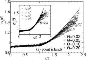
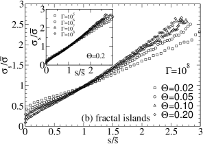
Figure 10: Scaled capture numbers $\sigma_{s}/\bar{\sigma}$ as function of the scaled island size $s/\bar{s}$ for fixed $\Gamma=10^{8}$ and four coverages $\Theta$, for (a) point and (b) fractal island morphologies. The insets show the scaled capture numbers at fixed $\Theta=0.2$ and the four simulated $\Gamma$ values. The line in (a) marks the solution obtained from a numerical integration of Eq. (11) when using the fit (line) to the scaled ISDs curve for $\Gamma=10^{8}$ and $\Theta=0.2$ in Fig. 9(a).

Figure 9 shows $n_{s}\bar{s}^{2}/\Theta$ as a function of $s/\bar{s}$ for $\Gamma=10^{8}$ at four different coverages for the (a) point and (b) fractal island morphologies. In the insets the scaled ISDs are shown for a fixed coverage $\Theta=0.2$ and different $\Gamma$. In the case of the point island morphologies, the data suggest the existence of a $\Theta$-independent limiting curve, in agreement with previous findings.Evans et al. (2006) For the fractal island morphologies, the scaled ISD for different $\Theta$ show no clear signature of a $\Theta$-independent limiting curve. Based on the tendency of the simulated data for different $\Theta$ and $\Gamma$ to become slightly closer to each other for larger $\Theta$ and $\Gamma$, one may conjecture that also in this case a limiting curve would be reached at larger $\Gamma$ values. However, the fact that for each fixed $\Theta$, the curves at large $\Gamma$ are almost overlapping suggests that these are good estimates of $f_{\infty}(x,\Theta)$. Our conclusion is therefore that it is not likely that a $\Theta$-independent limiting curve exists for the hit-and-stick model used here for the fractal island morphologies.

This conclusion is further corroborated by the fact that the scaled direct capture areas exhibit a nearly linear dependence on $x$ for the fractal islands (not shown). Thus we encounter the case here, where the scaled direct capture areas $\bar{\kappa}(\Theta,\Gamma)/\bar{s}(\Theta,\Gamma)$ appear to approach a non-vanishing limit for $\Gamma\to\infty$, which would mean that in a strict treatment, Eq. (7) can no longer be applied. If one considers $f_{\infty}(x,\Theta)$ to depend only very weakly on $\Theta$, $\partial f_{\infty}(x,\Theta)/\partial\Theta\simeq 0$, we could replace $C_{\infty}(x)$ by $C_{\rm tot}(x)=C_{\infty}(x)+\rho_{\infty}\Theta K_{\infty}(x,\Theta)/(1-\Theta)$, where $K_{\infty}(x,\Theta)=\lim_{\Gamma\to\infty}\kappa_{x\bar{s}}(\Theta,\Gamma)/\bar{\kappa}(\Theta,\Gamma)$ is the limiting curve for the scaled direct capture areas and $\rho_{\infty}=\lim_{\Gamma\to\infty}\bar{\kappa}(\Theta,\Gamma)/\bar{s}(\Theta,\Gamma)>0$.

Our conclusions drawn with respect to the scaled ISDs of the point islands are consistent with the behavior of the scaled capture numbers, which are shown in Fig. 10(a) for the same $\Theta$ and $\Gamma$ values as in Fig. 9(a). In this Fig. 10(a) an approach to a $\Theta$-independent limiting curve $C_{\infty}(x)$ can be seen. In the case of the fractal island morphologies by contrast, an approach to a $\Theta$-independent limiting curve cannot be clearly identified, which gives further evidence that the $f_{\infty}(x,\Theta)$ are dependent on $\Theta$.

In order to test the validity of Eq. (7) for the point islands, we set $z_{\infty}=2/3$ (see Sec. III) and used a fit to the scaled ISD for $\Gamma=10^{8}$ and $\Theta=0.2$ in Fig. 9(a) as an estimate for $f_{\infty}(x)$. The fit, which fulfills the constraints of normalization and normalized first moment, is shown as line in this figure. We then estimated $C_{\infty}(x)$ based on this fit by rewriting Eq. (17) from Appendix A (for $\Theta$-independent $f_{\infty}(x)$) in the form

$$\frac{\mathrm{d}C_{\infty}(x)}{\mathrm{d}x} =(2z_{\infty}-1)-[C_{\infty}(x)-z_{\infty}x]\frac{{\mathrm{d}}\ln(f_{\infty}(x))}{\mathrm{d}x}\,.$$ (11)

Since the solution of this differential equation is proportional to $1/f_{\infty}(x)$, we preferred to integrate Eq. (11) with the initial condition $C_{\infty}(0)=f_{\infty}(0)/(1-z_{\infty})$ to achieve a stable numerical results for large $x$ also. The resulting estimate for $C_{\infty}(x)$ is shown as line in Fig. 10(a). The line lies slightly above the data for the scaled capture numbers for $\Gamma=10^{8}$ and $\Theta=0.2$, indicating that indeed an estimate of a limiting curve for the scaled capture numbers is obtained. In a cross-check, we performed the integral in Eq. (7) with the estimated $C_{\infty}(x)$ and recovered the line in Fig. 9(a).

For the compact island morphologies, Eq. (7) would be of limited practical use, because, as discussed in Sec. V, the RE (I), (2) fail to predict the ISD correctly already at small $\Theta$ due to coalescences. Nevertheless, from a conceptual viewpoint, it is interesting to study the scaled ISD and their relation to the scaled capture numbers for the sub-islands. The corresponding data shown in Fig. 11 indicate a behavior similar as for the fractal island morphologies, where the limiting curves are dependent on $\Theta$.

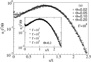
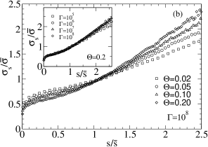
Figure 11: (a) Scaled island size distributions and (b) scaled capture numbers of sub-islands as function of the scaled island size in the case of compact island morphologies for fixed $\Gamma=10^{8}$ and four coverages $\Theta$. The inset shows the corresponding data at fixed $\Theta=0.2$ and the four simulated $\Gamma$ values.

VII Summary

The capture numbers entering the RE for the growth kinetics of thin films have been determined by KMC simulations in their dependence on both the coverage $\Theta$ and the $\Gamma=D/F$ ratio for the point island model and for two simple growth models representative for islands with compact and fractal shapes. It was shown that the $\Theta$-dependence of the capture numbers could not be accounted for by the ratio $R_{s}/\xi$ of the mean island radius $R_{s}$ and the effective adatom capture length $\xi$ of the RE. This suggests that the strong deviations between the capture numbers determined from the simulations and the ones predicted by the self-consistent theory have their origin in the linearization step used in this theory. The RE with self-consistent capture numbers nevertheless provide a good quantitative account of the adatom and island density. The deviations to the correct capture numbers lead, however, to a failure for a description of the ISD.

Integration of the RE with the simulated capture numbers determined from the KMC simulations gives an excellent quantitative prediction of the ISDs. For the compact islands morphologies, it was found that coalescence events, not considered in the RE, become relevant already at small coverages well below $\Theta\simeq 0.15$, where coalescence events do not significantly affect the island density. Compared to the fractal island morphologies, the coalescence rate for the compact morphologies is much higher. The ISD is affected already by a rather small number of coalescences, because these lead to a reshuffling of weights for different island sizes. The lower coalescence rate for fractal morphologies is caused by the fact that fingers of two approaching fractal islands typically first avoid each other, which subsequently leads to a screening effect and a slowing down of further growth of these fingers.

Finally we discussed the limiting curves for the scaled ISDs when $\Gamma\to\infty$. For the point islands the KMC data provide evidence that these limiting curves are independent of the coverage, which is given by the RE prediction (7). This means that there exists a true scaling behavior in the $\Gamma\to\infty$ limit, where the dependence on $\Theta$ is fully accounted for by the mean island size $\bar{s}$. For the growth models representing compact and fractal island morphologies, the results indicate that the limiting curves are dependent on $\Theta$. This implies that one needs to solve the partial differential equation (17) [or Eq. (21)] to calculate $f_{\infty}(x,\Theta)$ from $C_{\infty}(x,\Theta)$. Unfortunately no successful theory exists so far to predict the limiting curve $C_{\infty}(x,\Theta)$ for the scaled capture numbers.

The limiting curves are also different for different morphologies. Considering how sensitive the shape of the limiting curves depends on the nonlinear behavior of the scaled capture numbers as a function of the scaled island size, it is well possible that the shape will also vary with details of the growth mechanisms, even if the type of island morphology remains essentially the same.

Appendix A Rate equation prediction of the limiting curves for the scaled island size distribution

For large $\Gamma$, $\bar{s}\sim N^{-1}\sim\Gamma^{1/3}$ and $x=s/\bar{s}$ becomes a continuous variable, which allows one to derive a determining equation for the scaled ISD in dependence of the scaled capture numbers. The derivation was first presented by Bartelt and Evans.Bartelt and Evans (1996); Evans and Bartelt (2001) Replacing the variable $s$ by $x$ and using $\partial/\partial(Ft)=(1-\Theta)\partial/\partial\Theta$, Eqs. (2) can be written in the continuum limit as

$$\frac{\partial n_{x\bar{s}}}{\partial\Theta} =-\frac{1}{(1-\Theta)\bar{s}}\left\{\Gamma n_{1}\frac{\partial}{\partial x}\Big{(}\sigma_{x\bar{s}}n_{x\bar{s}}\Big{)}+\frac{\partial}{\partial x}\Big{(}\kappa_{x\bar{s}}n_{x\bar{s}}\Big{)}\right\}\,.$$ (12)

Defining $f(x,\Theta,\Gamma)=\bar{s}^{2}n_{x\bar{s}}/\Theta$, $C(x,\Theta,\Gamma)=\sigma_{x\bar{s}}/\bar{\sigma}$, and $K(x,\Theta,\Gamma)=\kappa_{x\bar{s}}/\bar{\kappa}$, one has

$$\frac{\partial}{\partial x}\Big{(}\sigma_{x\bar{s}}n_{x\bar{s}}\Big{)} =\frac{\Theta\bar{\sigma}}{\bar{s}^{2}}\frac{\partial(Cf)}{\partial x}$$ (13)

$$\frac{\partial}{\partial x}\Big{(}\kappa_{x\bar{s}}n_{x\bar{s}}\Big{)} =\frac{\Theta\bar{\kappa}}{\bar{s}^{2}}\frac{\partial(Kf)}{\partial x}$$ (14)

$$\frac{\partial n_{x\bar{s}}}{\partial\Theta} =-(2z-1)f-zx\frac{\partial f}{\partial x}+\Theta\frac{\partial f}{\partial\Theta}$$ (15)

where $z(\Theta,\Gamma)=\partial\ln\bar{s}/\partial\ln\Theta$. The reduced RE moreover predict $n_{1}\sim(1-\Theta)/(\Gamma\bar{\sigma}N)\sim(1-\Theta)\bar{s}/(\Theta\Gamma\bar{\sigma})$ for large $\Gamma$ and fixed $\Theta>\Theta_{x}\sim\Gamma^{-1/2}$. Inserting this relation and Eqs. (13, 14, 15) into Eq. (12) gives

$$(2z-1)f+zx\frac{\partial f}{\partial x}-\Theta\frac{\partial f}{\partial\Theta} =\frac{\partial(Cf)}{\partial x}+\frac{\Theta\bar{\kappa}}{(1-\Theta)\bar{s}}\frac{\partial(Kf)}{\partial x}$$ (16)

Introducing the limits $C_{\infty}(x,\Theta)=\lim_{\Gamma\to\infty}C(x,\Theta,\Gamma)$, $K_{\infty}(x,\Theta)=\lim_{\Gamma\to\infty}K(x,\Theta,\Gamma)$ and $z_{\infty}(\Theta)=\lim_{\Gamma\to\infty}z(\Theta,\Gamma)$, Eq. (16) yields a determining equation for $f_{\infty}(x,\Theta)=\lim_{\Gamma\to\infty}f(x,\Theta,\Gamma)$.

For $\lim_{\Gamma\to\infty}\bar{\kappa}/\bar{s}=0$ one obtains

$$(2z_{\infty}-1)f_{\infty}+z_{\infty}x\frac{\partial f_{\infty}}{\partial x}-\Theta\frac{\partial f_{\infty}}{\partial\Theta} =\frac{\partial(C_{\infty}f_{\infty})}{\partial x}$$ (17)

The condition $\lim_{\Gamma\to\infty}\bar{\kappa}/\bar{s}=0$ is valid for point islands, and it can be expected to hold also for compact island morphologies unless atoms deposited on top of islands are essentially all attaching to the island edge in the first layer (a situation unlikely due to second layer nucleation on larger islands).

When integrating Eq. (17) over $x$ from zero to infinity, the first, second and third term on the left hand side yield $(2z_{\infty}-1)$, $z_{\infty}$ (after a partial integration) and zero, respectively, because of the normalization of $f_{\infty}$. The right hand side becomes $[-C_{\infty}(0,\Theta)f_{\infty}(0,\Theta)]$ (note that for large $x$, $C_{\infty}\sim x$ and $f_{\infty}$ must decrease faster than $x$ to be normalizable – simulation results show that $f_{\infty}$ should in fact decay much faster). Accordingly, the relation

$$f_{\infty}(0,\Theta)=\frac{1-z_{\infty}(\Theta)}{C_{\infty}(0,\Theta)}$$ (18)

must be fulfilled. A corresponding relation can be derived in the same way already from Eq. (16). Analogously, when first multiplying Eq. (17) with $x$ and then integrating, one obtains

$$\int_{0}^{\infty}C_{\infty}(x,\Theta)f_{\infty}(x,\Theta)=1\,.$$ (19)

Integrating Eq. (17) to a finite value $x$ then yields

$$C_{\infty}(x,\Theta) =z_{\infty}(\Theta)x+\frac{1-z_{\infty}(\Theta)}{f_{\infty}(x,\Theta)}\int_{x}^{\infty}dx^{\prime}\,f_{\infty}(x^{\prime},\Theta)$$

$${}-\frac{\Theta}{f_{\infty}(x,\Theta)}\frac{\partial}{\partial\Theta}\int_{0}^{x}dx^{\prime}\,f_{\infty}(x^{\prime},\Theta)\,,$$ (20)

which expresses $C_{\infty}(x,\Theta)$ as a functional of $f_{\infty}(x,\Theta)$.

When one further assumes that the limiting curve $f_{\infty}$ is independent of $\Theta$, one has $\partial f_{\infty}/\partial\Theta=0$ and can neglect the corresponding term in Eq. (16). For self-consistency, this requires also $C_{\infty}$ and $z_{\infty}$ to become independent of $\Theta$. In fact, one can conversely show that if $C_{\infty}$ and $z_{\infty}$ are independent of $\Theta$, $f_{\infty}$ must by independent of $\Theta$ also. Under this assumption Eq. (17) then reduces to a separable ordinary differential equation, whose solution is given by Eq. (7), with $C_{\rm tot}(x)$ equal to $C_{\infty}(x)$ and $z$ equal to $z_{\infty}$.

If there exists a finite limit $\rho_{\infty}(\Theta)=\lim_{\Gamma\to\infty}\bar{\kappa}/\bar{s}>0$ , as it may be the case for fractal island morphologies (see the discussion in Sec. VI), Eq. (16) yields

$$(2z_{\infty}-1)f_{\infty} +z_{\infty}x\frac{\partial f_{\infty}}{\partial x}-\Theta\frac{\partial f_{\infty}}{\partial\Theta}=$$ (21)

$$\frac{\partial(C_{\infty}f_{\infty})}{\partial x}+\rho_{\infty}\frac{\Theta}{(1-\Theta)}\frac{\partial(K_{\infty}f_{\infty})}{\partial x}$$

as determining equation for $f_{\infty}(x,\Theta)$. Strictly speaking, a $\Theta$-independent $f_{\infty}(x)$ should not exist then and one needs to solve the semi-linear partial differential equation (21). If one nevertheless makes the approximation $\partial f_{\infty}/\partial\Theta\simeq 0$ in Eq. (21) and considers $C_{\infty}$ and $z_{\infty}$ to be independent of (or only weakly dependent on) $\Theta$, one would obtain the weakly $\Theta$-dependent solution Eq. (7) with $C_{\rm tot}=C_{\infty}+\rho_{\infty}\Theta K_{\infty}/(1-\Theta)$.

Figure 12: (a) Mean fraction $\Phi$ of distance vectors with anti-parallel orientation (with respect to the center of mass distance vector), and (b) mean minimal distance $d$ between islands as function of the time lag $\Delta t<0$ before a coalescence event at zero time. The times are given in units of $F^{-1}$ and the data were determined from the KMC simulations for $\Gamma=10^{7}$.

Appendix B Quantitative analysis of coalescence events

For a quantitative analysis of the coalescence behavior we determined the fraction of pair distance vectors of coalescing islands that before coalescence exhibit an anti-parallel orientation to the vector connecting the center of masses of the islands. Let us denote by $\mathbf{R}_{i,j}$ the vector pointing from the center of mass of island $i$ to the center of mass of island $j$, and by $\mathbf{r}_{i\alpha,j\beta}$ the vector pointing from atom $\alpha$ of island $i$ to atom $\beta$ of island $j$. The fraction of distance vectors with anti-parallel orientation then is

$$\Phi_{ij}=\frac{1}{s_{i}s_{j}}\sum_{\alpha,\beta}H(-\mathbf{r}_{i\alpha,j\beta}\cdot\mathbf{R}_{i,j})\,,$$ (22)

where $H(.)$ is the Heaviside jump function with $H(x)=1$ for $x>0$ and zero else. For a given time lag $\Delta t$ before coalescence, the $\Phi_{ij}$ were averaged over all coalescence events, yielding the mean fraction $\Phi(\Delta t)$ of distance vectors with anti-parallel orientation. To obtain the corresponding data, configurations generated by the KMC simulations were analyzed afterwards back in time, starting from the instant where islands first touched each other.

The mean fraction $\Phi$ obtained from this analysis is shown in Fig. 12(a) as a function of $\Delta t$ for $\Gamma=10^{7}$. We assigned negative values to $\Delta t$ to emphasize that $\Phi(\Delta t)$ was determined for lags before a coalescence event. That $\Phi(\Delta t)$ for fractal islands is by many orders of magnitude larger than for compact islands demonstrates the partial inter-penetration of the fractal islands before coalescence. The value $\Phi(\Delta t)\simeq 0.01$ reached for the fractal island morphologies in the limit $\Delta t\to 0$ means that on average about 10% of the atoms of each island in a coalescence event pass each other. That the partial inter-penetration is accompanied by a slowing down of the approach of two islands before coalescence can be seen in Figure 12(b), where the averaged minimal distance $d(\Delta t)$ between coalescing islands is shown, that means $d_{ij}=\min_{\alpha,\beta}(|\mathbf{r}_{i\alpha,j\beta}|)$ averaged over all coalescences of islands $i$ and $j$ for time lag $\Delta t$. The (negative) slope of $d(\Delta t)$ is significantly smaller for the fractal island morphologies, giving evidence for the screening effect.Brune (1998); Brune et al. (1999)

References

- Brune (1998) H. Brune, Surface Science Reports 31, 125 (1998).
- Michely and Krug (2004) T. Michely and J. Krug, Islands, Mounds and Atoms: Patterns and Processes in Crystal Growth far from equilibrium (Springer, Berlin, 2004).
- Evans et al. (2006) J. W. Evans, P. A. Thiel, and M. C. Bartelt, Surf. Sci. Rep. 61, 1 (2006).
- Dieterich et al. (2008a) W. Dieterich, M. Einax, and P. Maass, Eur. Phys. J. Special Topics 161, 151 (2008a).
- Venables (1973) J. A. Venables, Phil. Mag. 27, 697 (1973).
- Hlawacek et al. (2008) G. Hlawacek, P. Puschnig, P. Frank, A. Winkler, C. Ambrosch-Draxl, and C. Teichert, Science 321, 108 (2008).
- Loske et al. (2010) F. Loske, J. Lübbe, J. Schütte, M. Reichling, and A. Kühnle, Phys. Rev. B 82, 155428 (2010).
- Zangwill and Vvedensky (2011) A. Zangwill and D. D. Vvedensky, Nano Letters 11, 2092 (2011).
- Potocar et al. (2011) T. Potocar, S. Lorbek, D. Nabok, Q. Shen, L. Tumbek, G. Hlawacek, P. Puschnig, C. Ambrosch-Draxl, C. Teichert, and A. Winkler, Phys. Rev. B 83, 075423 (2011).
- Körner et al. (2011) M. Körner, F. Loske, M. Einax, A. Kühnle, M. Reichling, and P. Maass, Phys. Rev. Lett. 107, 016101 (2011).
- Ratsch and Venables (2003) C. Ratsch and J. A. Venables, J. Vac. Sci. Technol. A 21, S96 (2003).
- (12) When starting from a many-particle master equation for the growth kinetics of interacting adsorbate particles, the nonlinear terms in the rate equations would arise from some mean-field treatment of higher order correlation functions of occupations numbers, see, for example, J.-F. Gouyet et al., Adv. Phys. 52, 523 (2003).
- Körner et al. (2010) M. Körner, M. Einax, and P. Maass, Phys. Rev. B 82, 201401 (2010).
- Bales and Chrzan (1994) G. S. Bales and D. C. Chrzan, Phys. Rev. B 50, 6057 (1994).
- Bales and Zangwill (1997) G. S. Bales and A. Zangwill, Phys. Rev. B 55, R1973 (1997).
- Bartelt and Evans (1996) M. C. Bartelt and J. W. Evans, Phys. Rev. B 54, R17359 (1996).
- Evans and Bartelt (2001) J. W. Evans and M. C. Bartelt, Phys. Rev. B 63, 235408 (2001).
- Venables et al. (1984) J. A. Venables, G. D. T. Spiller, and M. Hanbucken, Rep. Prog. Phys. 47, 399 (1984).
- Venables (1994) J. A. Venables, Surface Science 299-300, 798 (1994).
- Einax et al. (2007) M. Einax, S. Ziehm, W. Dieterich, and P. Maass, Phys. Rev. Lett. 99, 016106 (2007).
- Einax et al. (2009) M. Einax, W. Dieterich, and P. Maass, J. Appl. Phys. 105, 054312 (2009).
- Vicsek and Family (1984) T. Vicsek and F. Family, Phys. Rev. Lett. 52, 1669 (1984).
- Vvedensky (2000) D. D. Vvedensky, Phys. Rev. B 62, 15435 (2000).
- Amar and Family (1995) J. G. Amar and F. Family, Phys. Rev. Lett. 74, 2066 (1995).
- Ruiz et al. (2003) R. Ruiz, B. Nickel, N. Koch, L. C. Feldman, R. F. Haglund, A. Kahn, F. Family, and G. Scoles, Phys. Rev. Lett. 91, 136102 (2003).
- Pomeroy and Brock (2006) J. M. Pomeroy and J. D. Brock, Phys. Rev. B 73, 245405 (2006).
- Pimpinelli and Einstein (2007) A. Pimpinelli and T. L. Einstein, Phys. Rev. Lett. 99, 226102 (2007).
- Oliveira and Aarão Reis (2011) T. J. Oliveira and F. D. A. Aarão Reis, Phys. Rev. B 83, 201405 (2011).
- Li et al. (2010) M. Li, Y. Han, and J. W. Evans, Phys. Rev. Lett. 104, 149601 (2010).
- Pimpinelli and Einstein (2010) A. Pimpinelli and T. L. Einstein, Phys. Rev. Lett. 104, 149602 (2010).
- Gibou et al. (2001) F. G. Gibou, C. Ratsch, M. F. Gyure, S. Chen, and R. E. Caflisch, Phys. Rev. B 63, 115401 (2001).
- Gibou et al. (2003) F. Gibou, C. Ratsch, and R. Caflisch, Phys. Rev. B 67, 155403 (2003).
- Gyure et al. (1998) M. F. Gyure, C. Ratsch, B. Merriman, R. E. Caflisch, S. Osher, J. J. Zinck, and D. D. Vvedensky, Phys. Rev. E 58, R6927 (1998).
- Bartelt et al. (1999a) M. C. Bartelt, C. R. Stoldt, C. J. Jenks, P. A. Thiel, and J. W. Evans, Phys. Rev. B 59, 3125 (1999a).
- Bartelt et al. (1998) M. C. Bartelt, A. K. Schmid, J. W. Evans, and R. Q. Hwang, Phys. Rev. Lett. 81, 1901 (1998).
- Hannon et al. (1998) J. B. Hannon, M. C. Bartelt, N. C. Bartelt, and G. L. Kellogg, Phys. Rev. Lett. 81, 4676 (1998).
- Brune et al. (1999) H. Brune, S. Bales, J. Jacobsen, C. Boragno, and K. Kern, Phys. Rev. B. 60, 5991 (1999).
- Holubec et al. (2011) V. Holubec, P. Chvosta, M. Einax, and P. Maass, Europhys. Lett. 93, 40003 (2011).
- Gillespie (1977) D. T. Gillespie, J. Phys. Chem. 81, 2340 (1977).
- Bartelt and Evans (1993) M. C. Bartelt and J. W. Evans, Surface Science 298, 421 (1993).
- Bartelt et al. (1999b) M. C. Bartelt, C. R. Stoldt, C. J. Jenks, P. A. Thiel, and J. W. Evans, Phys. Rev. B 59, 3125 (1999b).
- Amar et al. (2001) J. G. Amar, M. N. Popescu, and F. Family, Phys. Rev. Lett. 86, 3092 (2001).
- Bartelt and Evans (1992) M. C. Bartelt and J. W. Evans, Phys. Rev. B 46, 12675 (1992).
- Dieterich et al. (2008b) W. Dieterich, M. Einax, S. Heinrichs, and P. Maass, “Fluctuation effects in kinetic thin film growth,” in Anomalous Fluctuation Phenomena in Complex Systems: Plasmas, Fluids, and Financial Markets, edited by C. Riccardi and H. E. Roman (Transworld Research Network, Kerala, India, 2008) Chap. 8, pp. 211–244.
- Popescu et al. (2001) M. N. Popescu, J. G. Amar, and F. Family, Phys. Rev. B 64, 205404 (2001).
- Mulheran and Robbie (2000) P. A. Mulheran and D. A. Robbie, Europhys. Lett. 49, 617 (2000).
- Evans and Bartelt (2002) J. W. Evans and M. C. Bartelt, Phys. Rev. B 66, 235410 (2002).
- Mulheran (2004) P. A. Mulheran, Europhys. Lett. 65, 379 (2004).
- (49) M. Einax, W. Dieterich and P. Maass, to be published.