Generalized Metropolis dynamics with a generalized master equation: An approach for time-independent and time-dependent Monte Carlo simulations of generalized spin systems

Abstract

The extension of Boltzmann-Gibbs thermostatistics, proposed by Tsallis, introduces an additional parameter $q$ to the inverse temperature $\beta$. Here, we show that a previously introduced generalized Metropolis dynamics to evolve spin models is not local and does not obey the detailed energy balance. In this dynamics, locality is only retrieved for $q=1$, which corresponds to the standard Metropolis algorithm. Non-locality implies in very time consuming computer calculations, since the energy of the whole system must be reevaluated, when a single spin is flipped. To circumvent this costly calculation, we propose a generalized master equation, which gives rise to a local generalized Metropolis dynamics that obeys the detailed energy balance. To compare the different critical values obtained with other generalized dynamics, we perform Monte Carlo simulations in equilibrium for Ising model. By using the short time non-equilibrium numerical simulations, we also calculate for this model: the critical temperature, the static and dynamical critical exponents as function of $q$. Even for $q\neq 1$, we show that suitable time evolving power laws can be found for each initial condition. Our numerical experiments corroborate the literature results, when we use non-local dynamics, showing that short time parameter determination works also in this case. However, the dynamics governed by the new master equation leads to different results for critical temperatures and also the critical exponents affecting universality classes. We further propose a simple algorithm to optimize modeling the time evolution with a power law considering in a log-log plot two successive refinements.

I Introduction

The study of the critical properties of magnetic systems plays an important role in statistical mechanics and as a consequence also in thermodynamics. For equilibrium, the extensitivity of the entropy is a question of principle for most physicists. Nevertheless, an important issue may be raised. While many physicists believe that statistical mechanics generalizations with an extra parameter $q$ tsallis_1 are suitable to study the optimization combinatorial process as for example the simulated annealing (see e.g. Stariolo ,Uli1997 ), or areas such as econophysics martinez1 ; martinez2 , population dynamics and growth models martinez3 ; martinez4 ; martinez5 ; martinez6 , Bibliometry martinez7 and others.

In this paper, we generate the critical dynamics of Ising systems using a new master equation. This master equation leads to a generalized Metropolis prescription, which depends only on the spin interaction energy variations with respect to its neighborhood. Furthermore, it satisfies the detailed energy balance condition and it converges asymptotically to the generalized Boltzmann-Gibbs weights. In Refs. Crokidakis2009 ; Boer2011 generalized prescriptions have been treated as local. Here, we demonstrate that they are instead non-local. However, a non-local prescription such as the one of Ref. Penna1999 is numerically more expensive and destroys the phase transition. Another possibility is to recover locality. Using a special deformation of the master equation, we show how to recover locality for a generalized prescription and additionally recovering the detailed energy balance in equilibrium spin systems, maintaining the system phase transition.

To apply our Metropolis prescription, we have simulated a two dimensional Ising system in two different ways: using equilibrium Monte Carlo (MC) simulations we estimate critical temperatures for different $q$-values and performing time-dependent simulations. In the second part, we also calculate the critical exponents set corresponding to each critical temperature.Finally, we have developed an alternative methodology to refine the determination of the critical temperature. Our approach is based on the optimization of the magnetization power laws in log scale via of maximization of determination coefficient ($r$) of the linear fits.

Our presentation is organized as follows. In Sec. II, we briefly review the results of the critical dynamics for spins systems. In this review, we calculate the critical exponents for the several spin phases, that emerge from different initial conditions. In Sec. III, we propose a new master equation that leads to a Metropolis algorithm, which preserves locality and detailed energy balance, also for $q\neq 1$. In Sec. IV, we simulate an equilibrium Ising spin system in a square lattice and show the differences between the results of our approach and of Refs. Crokidakis2009 ; Boer2011 . Next, we evolve a Ising spin system in a square lattice, from ordered and disordered initial conditions in the context of time dependent simulations. From such non equilibrium Monte Carlo simulations, also called short time simulations, we are able to calculate the dynamic and static critical exponents ones. Finally, the conclusions are presented in Sec. V.

II Critical dynamics of spin systems and time dependent simulations

Here, we briefly review finite size scaling in the dynamics relaxation of spin systems. We present our alternative deduction of the some expected power laws in the short time dynamics context. Readers, which want a more complete review about this topic, may want to read Zheng1998 .

This topic is based on time dependent simulations, and it constitutes an important issue in the context of phase transitions and critical phenomena. Such methods can be applied not only to estimate the critical parameters in spin systems, but also to calculate the critical exponents (static and dynamic ones) through different scaling relations by setting different initial conditions.

The study of the statistical systems dynamical critical properties has become simpler in nonequilibrium physics after the seminal ideas of Janssen, Schaub and Schmittmann Janssen1989 and Huse Huse1989 . quenching systems from high temperatures to the critical one, they have shown universality and scaling behavior to appear already in the early stages of time evolution, via renormalization group techniques and numerical calculations respectively. Hence, using short time dynamics, one can often circumvent the well-known problem of the critical slowing down that plagues investigations of the long-time regime.

The dynamic scaling relation obtained by Janssen et al. for the magnetization k-th moment, extended to finite size systems, is written as

$$\langle M^{k}\rangle(t,\tau,L,m_{0})=b^{-k\beta/\nu}\langle M^{k}\rangle(b^{-z}t,b^{1/\nu}\tau,b^{-1}L,b^{x_{0}}m_{0})\text{,}$$ (1)

where the arguments are: the time $t$; the reduced temperature $\tau=(T-T_{c})/T_{c}$, with $T_{c}$ being the critical one, the lattice linear size $L$ and initial magnetization $m_{0}$. Here, the operator $\langle\ldots\rangle$ denotes averages over different configurations due to different possible time evolution from each initial configuration compatible with a given $m_{0}$. On the equation right-hand-side, one has: an arbitrary spatial rescaling factor $b$; an anomalous dimension $x_{0}$ related to $m_{0}$. The exponents $\beta$ and $\nu$ are the equilibrium critical exponents associated with the order parameter and the correlation length, respectively. The exponent $z$ is the dynamic one, which characterizes the time correlations in equilibrium. After the scaling $b^{-1}L=1$ and at the critical temperature $T=$ $T_{c}$, the first ($k=1$) magnetization moment is: $\langle M\rangle(t,L,m_{0})=L^{-\beta/\nu}\langle M\rangle(L^{-z}t,L^{x_{0}}m_{0})$.

Denoting $u=tL^{-z}$ and $w=L^{x_{0}}m_{0}$, one has: $\langle M\rangle(u,w)=\langle M\rangle(L^{-z}t,L^{x_{0}}m_{0})$. The derivative with respect to $L$ is: $\partial_{L}\langle M\rangle=(-\beta/\nu)L^{-\beta/\nu-1}\langle M\rangle(u,w)+L^{-\beta/\nu}[\partial_{u}\langle M\rangle\partial_{L}u+\partial_{w}\langle M\rangle\partial_{L}w]$, where we have explicitly: $\partial_{L}u=-ztL^{-z-1}$ and $\partial_{L}w=x_{0}m_{0}L^{x_{0}-1}$. In the limit $L\rightarrow\infty$, $\partial_{L}\langle M\rangle\rightarrow 0$, one has: $x_{0}w\partial_{w}\langle M\rangle-zu\partial_{u}\langle M\rangle-\beta/\nu\langle M\rangle=0$. The separability of the variables $u$ and $w$ in $\langle M\rangle(u,w)=M_{1}(u)M_{2}(w)$ leads to $x_{0}wM_{2}^{\prime}/M_{2}=\beta/\nu+zuM_{1}^{\prime}/M_{2}$, where the prime means the derivative with respect to the argument. Since this equation left-hand-side depends only on $w$ and the right-hand-side depends only on $u$, they must be equal to a constant $c$. Thus, $M_{1}(u)=u^{(c/z)-\beta/(\nu z)}$ and $M_{2}(w)=w^{c/x_{0}}$, resulting in $\left\langle M\right\rangle(u,w)=m_{0}^{c/x_{0}}L^{\beta/\nu}t^{(c-\beta/\nu)/z}$. Returning to the original variables, one has: $\langle M\rangle(t,L,m_{0})=m_{0}^{c/x_{0}}t^{(c-\beta/\nu)/z}$.

On one hand, choosing $c=x_{0}$ and calculating $\theta=(x_{0}-\beta/\nu)/z$, at criticality ($\tau=0$), we obtain $\langle M\rangle_{m_{0}}\sim m_{0}t^{\theta}$ corresponding to a regime under small initial magnetization. This can be observed by a finite time scaling $b=t^{1/z}$ in equation 1, at critical temperature ($\tau=0$) which leads to $\left\langle M\right\rangle(t,m_{0})=t^{-\beta/(\nu z)}\langle M\rangle(1,t^{x_{0}/z}m_{0})$. Defining $x=t^{x_{0}/z}m_{0}$, an expansion of the averaged magnetization around $x=0$ results in: $\langle M\rangle(1,x)=\langle M\rangle(1,0)+\left.\partial_{x}\langle M\rangle\right|_{x=0}x+\mathcal{O}(x^{2})$. By construction $\langle M\rangle(1,0)=0$, since $u=t^{x_{0}/z}m_{0}\ll 1$ and $\left.\partial_{x}\langle M\rangle\right|_{x=0}$ is a constant. So, by discarding the quadratic terms we obtain the expected power law behavior $\langle M\rangle_{m_{0}}\sim m_{0}t^{\theta}$. This anomalous behavior of initial magnetization is valid only for a characteristic time scale $t_{\max}$ $\sim m_{0}^{-z/x_{0}}$.

On the other hand, the choice $c=0$ corresponds to a case where the system does not depend on the initial trace of the system; and $m_{0}=1$ leads to simple power law:

$$\langle M\rangle_{m_{0}=1}\sim t^{-\beta/(\nu z)}$$ (2)

that similarly corresponds to decay of magnetization for $t>t_{\max}$ of a system that previously evolved from a initial small magnetization $(m_{0})$, and had its magnetization increased up to a magnetization peak.

For $m_{0}=0$, it is not difficult to show that the magnetization second moment is

$$\left\langle M^{2}\right\rangle_{m_{0}=0}\sim t^{(d-2\beta/\nu)/z}\;,$$ (3)

where $d$ is the system dimension.

Using Monte Carlo simulations, many authors have obtained the dynamic exponents $\theta$ and $z$ as well as the static ones $\beta$ and $\nu$, and other specific exponents for many different models and situations: Baxter-Wu Arashiro2003 , 2, 3 and 4-state Potts daSilva2002a ; daSilva2004 , Ising with multispin interactions Simoes2001 , models with no defined Hamiltonian (celular automata and contact process) daSilva2004a ; tome1998 ; daSilva2005 , models with tricritical point daSilva2002 , Heisenberg Fernandes2006 , protein folding Arashiro2 ; Arashiro3 , propagation of damages in Ising models albano2010 .

The sequence to determine the static exponents from short time dynamics is: to determine $z$ first, performing Monte Carlo simulations that mixes initial conditions daSilva2002a , and consider the power law for the cumulant

$$F_{2}(t)=\frac{\left\langle M^{2}\right\rangle_{m_{0}=0}}{\left\langle M\right\rangle_{m_{0}=1}^{2}}\sim t^{d/z}\;.$$ (4)

Once $z$ is calculated, the exponent $\eta=2\beta/\nu$ is calculated according to $\eta=2\widehat{(\beta/\nu z)}\cdot\widehat{z}$, where $\widehat{(\beta/\nu z)}$ was estimated via magnetization decay and $\widehat{z}$ from cumulant $F_{2}$.

However, prior to obtaining the critical exponents, we also perform time dependent MC simulations in order to refine the critical temperatures. These are based on power laws obtained by finite size scaling analysis of the magnetization decay from an initially ordered state (Eq. 2). This choice demands a number of runs smaller than other power laws in non-equilibrium, and so we propose an simple algorithm that spans different critical values to find the best determination coefficient in linear fit $\ln\langle M\rangle$ versus $\ln t$ . This procedure is explored in Sec. IV, and is used later to calculate the critical temperatures for Ising models with different values of the non-extensivity parameter $q$ in our new Metropolis prescription.

III Generalized master equation

In this section, we start recalling the way that the Metropolis algorithm is obtained from the master equation for spin systems. We point out that the energy difference by flipping an Ising spin is local,i.e. it depends only on the flipped spin. Next, we show a first attempt to generalize the Metropolis algorithm Crokidakis2009 ; Boer2011 , according to the non-extensive thermostatistics, introduced by Tsallis tsallis_1 . We show that this generalization does not preserve the spin flip locality. To recover this locality, we propose a new generalized master equation, which leads to a different generalization of the Metropolis algorithm.

III.1 Standard master equation and Metropolis algorithm

In general, spin systems non-equilibrium dynamics are described by the time evolution of the probability $P(E,t)$ that, at instant $t$, the system has an energy $E$. This probability is obtained from the master equation: $dP(E^{(a)},t)/dt=\sum\limits_{\sigma_{i}^{(b)}}\{w[\sigma_{i}^{(b)}\rightarrow\sigma_{i}^{(a)}]P[E^{(b)},t]-w[\sigma_{i}^{(a)}\rightarrow\sigma_{i}^{(b)}]P[E^{(a)},t]\}$, where $w[\sigma_{i}^{(b)}\rightarrow\sigma_{i}^{(a)}]$ is the transition rate of the $i-$th spin from $\sigma_{i}^{(b)}$ to $\sigma_{i}^{(a)}$. Here, $E^{(b)}$ ($E^{(a)}$) is the energy of the system before (after) the transition. As $t\rightarrow\infty$, $dP(E,t)/dt=0$ is a necessary condition for equilibrium. A sufficient but not necessary condition for equilibrium, known as detailed balance condition, supposes a more restricted situation for ocurrence of $dP(E,t)/dt=0$, i.e., $w[\sigma_{i}^{(b)}\rightarrow\sigma_{i}^{(a)}]P[E^{(b)}]-w[\sigma_{i}^{(a)}\rightarrow\sigma_{i}^{(b)}]P[E^{(a)}]=0$, meaning that each term in the summation vanishes. In this case, $P(E)=P(E,t\rightarrow\infty)$ is the Boltzmann distribution: $P(E_{j})=e^{-\beta E_{j}}/\sum_{k}e^{-\beta E_{k}}$, where the summation is over the different energy states and $\beta=(k_{B}T)^{-1}$.

Employing detailed balance requires to find simple prescriptions for spins systems dynamics, as for example the Metropolis prescription: $w[\sigma_{i}^{(b)}\rightarrow\sigma_{i}^{(a)}]=\min\{1,\exp[-\beta(E^{(a)}-E^{(b)})]\}$. When applied to evolve spin systems, this simple dynamics reduce to calculate just local energy changes. For instance, the Ising model in two dimensions has an energy $E^{(b)}=-J\sigma_{i_{x},i_{y}}^{(b)}S_{i_{x},i_{y}}+\xi$ before the flip of spin $\sigma_{i_{x},i_{y}}$, located at site indexed by $i_{x}$ and $i_{y}$, where the local energy change is quantified by

$$S_{i_{x},i_{y}}=\sigma_{i_{x}+1,i_{y}}+\sigma_{i_{x}-1,i_{y}}+\sigma_{i_{x},i_{y}-1}+\sigma_{i_{x},i_{y}+1}$$

and the non-local energy is $\xi$, which is obtained excluding the spin $\sigma_{i_{x},i_{y}}$, from the calculation. After the spin flip, the energy is $E^{(a)}=-J\sigma_{i_{x},i_{y}}^{(a)}S_{i_{x},i_{y}}+\xi$ and the energy change of the system, due to the spin $\sigma_{i_{x},i_{y}}$ flip is simply:

$$E^{(a)}-E^{(b)}=-J[\sigma_{i_{x},i_{y}}^{(a)}-\sigma_{i_{x},i_{y}}^{(b)}]S_{i_{x},i_{y}}\;,$$ (5)

which does not depend on the energy of the other spins.

III.2 Generalized Metropolis algorithm

The system equilibrium is described by the generalized Boltzmann-Gibbs distribution

$$P_{1-q}(E_{i})=\frac{[e_{1-q}(-\beta^{\prime}E_{i})]^{q}}{\sum_{i=1}^{\Omega}[e_{1-q}(-\beta^{\prime}E_{i})]^{q}}\;,$$ (6)

where $\Omega$ is the number of accessible states of the system and $\beta^{\prime}=\beta/\sum\limits_{i=1}^{\Omega}\{[e_{1-q}(-\beta E_{i})]^{q}+(1-q)\beta\langle E\rangle_{1-q}\}$, where $\langle E\rangle_{1-q}=\sum\nolimits_{i=1}^{\Omega}E_{i}P_{1-q}(E_{i})$. Here it is important to mention that $(k_{B}\beta^{\prime})^{-1}$ is a scale temperature that can be used to interpret experimental and computational experiments. There is a heated ongoing discussion whether it is the physical temperature or not.

The function

$$e_{\alpha}(x)=\left\{\begin{array}[]{ll}(1+\alpha x)^{1/\alpha}&\mbox{for}\;\alpha x>-1\\ 0&\mbox{otherwise}\;,\end{array}\right.$$ (7)

is the generalized exponential tsallis_2 ; tiago . For $\alpha\rightarrow 0$, one retrieves the standard exponential function $e_{0}(x)=e^{x}$. It is this singularity at $\alpha x>-1$ that brings up interesting effects such the survival/extinction transitions in one-species population dynamical models martinez5 . The inverse of the generalized exponential function is the generalized logarithmic function $\ln_{\alpha}(x)=(x^{\alpha}-1)/\alpha$, which for $\alpha\rightarrow 0$ leads to the standard logarithm function $\ln_{0}(x)=\ln(x)$. Notice that the inequality $\alpha x>-1$, for fixed $x$ produces a limiting value for $\alpha$. This generalized logarithmic function has been introduced first in the context on non-extensive thermostatistics tsallis_1 ; tsallis_2 and has a clear geometrical interpretation ss the area between 1 and $x$ underneath the non-symmetric hyperbole $1/t^{1-\alpha}$ tiago . It is interesting to notice, that in 1984 Cressie and Read cressie proposed an entropy that would lead to a generalization of the logarithm function given by : $\ln_{\alpha}(x)/(\alpha+1)$. In this case, we would gain the limiting value in $\alpha$ but lose its geometrical interpretation.

To recover the additive property of the argument, when multiplying two generalized exponential functions: $e_{\alpha}(a)e_{\alpha}(b)=e_{\alpha}(a\oplus_{\alpha}b)$ [$e_{\alpha}(a)/e_{\alpha}(b)=e_{\alpha}(a\ominus_{\alpha}b)$] and $e_{\alpha}(a)\otimes_{\alpha}e_{\alpha}(b)=e_{\alpha}(a+b)$ [$e_{\alpha}(a)\oslash_{\alpha}e_{\alpha}(b)=e_{\alpha}(a-b)$] consider the following algebraic operators nivanen ; borges :

$$a\oplus_{\alpha}b = a+b+\alpha ab$$ (8)

$$a\ominus_{\alpha}b = \frac{a-b}{1+\alpha b}$$ (9)

$$a\otimes_{\alpha}b = \left(a^{\alpha}+b^{\alpha}-1\right)^{1/\alpha}$$ (10)

$$a\oslash_{\alpha}b = \left(a^{\alpha}-b^{\alpha}+1\right)^{1/\alpha}\;.$$ (11)

Observe that, if $a\ominus_{\alpha}b=0$, then $a=b$ and if $a\otimes_{\alpha}b=c\otimes_{\alpha}d$, then $a\oslash_{\alpha}c=d\oslash_{\alpha}b$.

However, in equilibrium, the Ising model prescribes an adapted Metropolis dynamics that considers a generalized version of exponential function Crokidakis2009 ; Boer2011 :

$$w[\sigma_{i}^{(b)}\rightarrow\sigma_{i}^{(a)}]=\frac{P_{1-q}[E^{(a)}]}{P_{1-q}[E^{(b)}]}=\left\{\frac{e_{1-q}[-\beta^{\prime}E^{(a)}]}{e_{1-q}[-\beta^{\prime}E^{(b)}]}\right\}^{q}\;.$$ (12)

From the generalization of the exponential function in the Boltzmann-Gibbs weight, the transition rate of Eq. 12 can be used to determine the system evolution, as the Metropolis algorithm. Nevertheless, we stress that in such a choice, the dynamics is not local. Because generalized exponential functions are non-additive, a spin flip introduces a change in the system energy that is spread all over the lattice. More precisely, consider the Ising model in a square lattice, one can show that:

$$\frac{e_{1-q}[-\beta^{\prime}E^{(a)}]}{e_{1-q}[-\beta^{\prime}E^{(b)}]}=e_{1-q}\{-\beta^{\prime}[E^{(a)}\ominus_{1-q}E^{(b)}]\}$$ (13)

or:

$$\frac{e_{1-q}[-\beta^{\prime}E^{(a)}]}{e_{1-q}[-\beta^{\prime}E^{(b)}]}\neq e_{1-q}\{-\beta^{\prime}[E^{(a)}-E^{(b)}]\}\;,$$ (14)

where $E^{(a)}-E^{(b)}$ is given by Eq. 5, which depends only the spins that directly interact with the flipped spin, violating the detailed energy balance.

In Refs Crokidakis2009 ; Boer2011 , the authors consider (with no explanations) the equality in Eq. 14, instead of considering Eq. 13. Thus, the detailed energy balance is violated, since the system is updated following a local calculation of the generalized Metropolis algorithm of Eq. 12.

To correct this problem, one must update the spin system using the non-locality of Eq. 12, which is numerically expensive, since the energy of the whole lattice must be recalculated due to a simple spin flip. The other alternative is to require that the transition rate depends locally in the energy difference of a simple spin flip, which in turn leads us to a modified master equation. Since the former is very expensive numerically, we explore only the latter alternative which is numerically faster and is able to produce statistically significant results for fairly large spin systems.

III.3 Recovering locality in the generalized Metropolis algorithm

Based on the operators of Eq. 8 to Eq. 11, we propose the following generalized master equation:

$$\frac{dP_{1-q}[E^{(a)}]}{dt}=\sum\limits_{\sigma_{i}^{(b)}} w[\sigma_{i}^{(b)}\rightarrow\sigma_{i}^{(a)}]\otimes_{\tilde{q}/q}P_{q}[E^{(b)}]\;\ominus_{\tilde{q}/q}$$ (15)

$$w[\sigma_{i}^{(a)}\rightarrow\sigma_{i}^{(b)}]\otimes_{\tilde{q}/q}P_{q}[E^{(a)}]\;.$$

where $P_{q}(E)$ is given by Eq. 6. Here, it is suitable to call $\tilde{q}=1-q$ and write the generalized exponentials as a function of $\tilde{q}$. In equilibrium, $dP_{1-q}/dt=0$ and a dynamics governed by Eq 6.

The detailed balance (a sufficient condition to equilibrium) for the generalized master equation is

$$w[\sigma_{i}^{(b)}\rightarrow\sigma_{i}^{(a)}]\oslash_{\tilde{q}/q}w[\sigma_{i}^{(a)}\rightarrow\sigma_{i}^{(b)}]=P_{q}[E^{(a)}]\oslash_{\tilde{q}/q}P_{q}[E^{(b)}]\;,$$ (16)

which leads to a new generalized Metropolis algorithm:

$$w(\sigma_{i}^{(b)}\rightarrow\sigma_{i}^{(a)}) = \min\left\{1,\left[e_{\tilde{q}}(-\beta^{\prime}E^{(a)})\right]^{q}\oslash_{\tilde{q}/q}\left[e_{\tilde{q}}(-\beta^{\prime}E^{(b)})\right]^{q}\right\}=\min\left\{1,\left[e_{\tilde{q}}(-\beta^{\prime}(E^{(a)}-E^{(b)}))\right]^{q}\right\}$$ (17)

$$= \min\left\{1,\left[e_{\tilde{q}}(\beta^{\prime}J\left[\sigma^{(a)}_{i_{x},i_{y}}-\sigma^{(b)}_{i_{x},i_{y}}\right]S_{i_{x},i_{y}})\right]^{q}\right\}$$

and now the transition probability depends only on energy between the read site and its neighbors, i.e., locality is retrieved.

IV Generalized Metropolis Algorithm – Numerical Simulation results

We have performed Monte Carlo simulations of the square lattice Ising model in the context of generalized Boltzmann-Gibbs weights. These simulations are based on two approaches for Metropolis dynamics. The first one (Metropolis I) is described in Ref. Crokidakis2009 , where the nonlocal transition rate of Eq. (12) is used to update the spin system. In the second approach (Metropolis II), the local transition rate of Eq. 17 is used. We separate our results in two different subsections: the equilibrium simulations and short time critical dynamics.

IV.1 Equilibrium

In this part we analyze the magnetization $\left\langle m\right\rangle$, where $\left\langle\cdot\right\rangle$ denotes averages under Monte Carlo (MC) steps. We perfom MC simulations for $q=0.6$, $q=0.8$ and $q=1.0$. In the simulations, we have used $L_{\min}=2^{4}=16$ up to $L_{\max}=2^{9}=512$, with periodic boundary conditions and a random initial configuration of the spins with $\left\langle m_{0}\right\rangle=0$. Differently from reported in Ref. Crokidakis2009, , where the results have been obtained after $10^{7}$ MC steps per spin, we have used $6.1^{3}$ MC steps per spin, an equilibrium situation consistent with the one reported by Newman and Barkema Newman1999 . This results in $1.5\cdot 10^{6}-1.5\cdot 10^{9}$ MC steps for the whole lattice of $16^{2}$ up to $512^{2}$ spins.

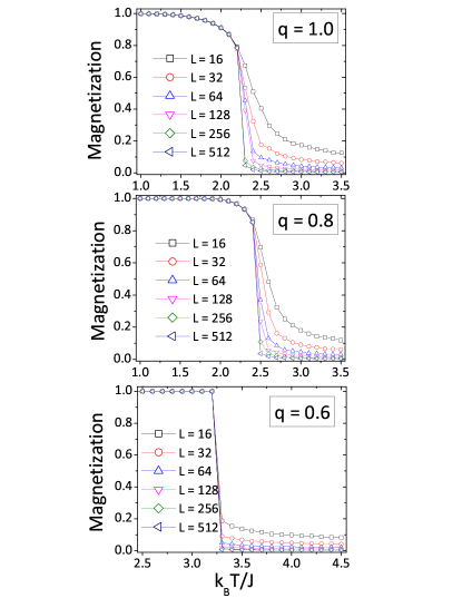
Figure 1: System magnetization versus temperature for $q=1.0$, 0.8 and 0.6. Using the dynamics based on Metropolis II, we observe phase transitions for critical values upper to $\log(1+\sqrt{2})/2$ as $q<1$ differently from previous studies, which are based on Metropolis I.

Fig. 1 shows the magnetization curves as function of critical temperature for different $q$-values. The critical temperature increases as $q$ decreases. This behavior, using our algorithm (Metropolis II) differs from the one obtained using the algorithm of Refs. Crokidakis2009, and Boer2011, (Metropolis I). We stress that both algorithms agree for $q=1$, the usual Boltzmann-Gibbs weights, converging to the theoretical value $\log(1+\sqrt{2})/2$. In Table 1, we show the critical temperature and error obtained from the extrapolation $L\rightarrow\infty$ (see Fig. 2) using both algorithms. These results suggest a thorough difference among the processes and critical values found between two the dynamics Metropolis I and II. In Fig. 1, the curves show phase transitions for critical values upper to $\log(1+\sqrt{2})/2$ as $q<1$. This differs from previous studies, which are based on prescription Metropolis I.

Fig. 1 shows that, differently from the $q=0.8$ and $q=1.0$ cases, for $q=0.6$ the discontinuity in the magnetization curve does not depend on system size $L$. In fact, in this case, the critical temperature $T_{c}$ does not depend on $L$. This effect occurs due to the cutoff of the escort probability distribution as reported for Metropolis I Crokidakis2009 for $q<0.5$. For Metropolis II, Fig. 2 depicts that $T_{c}$ remains constant for all values of $L^{-1}$, for $q=0.6$. For both cases, $q=1.0$ (obviously) and $q=0.8$, we have verified that $\nu\approx 1$ and $\beta\approx 0.125$, obtained from the collapse of the curves $\left\langle M\right\rangle L^{\beta/\nu}$ versus $(T-T_{c})L^{1/v}$. This data collapse permits the extrapolation of $k_{B}T_{c}/J$ versus $L^{-1}$, since $\nu\approx 1$ for both cases according to Fig. 2. In following, we show using non-equilibrium simulations that $2\beta/\nu\approx 0.25$, for $q=1$ and $q=0.8$, validating the data collapse results (see table 5).

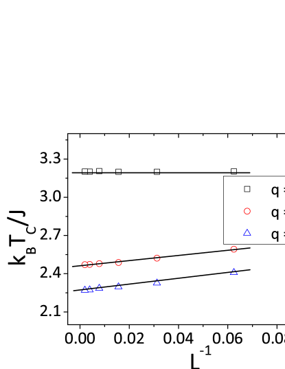
Figure 2: Extrapolation ($L\rightarrow\infty$) of critical temperatures for different $q-$values: $0.6,0.8$ and $1.0$ for the 2d Ising model.

$q$	ref. Metropolis I	Metropolis II
0.6	1.761(3)	3.201(1)
0.8	1.891(7)	2.461(5)
1.0	2.259(11)	2.262(9)

Table 1: Comparison between critical the critical temperature and error, for the 2d Ising model, obtained from extrapolation $L\rightarrow\infty$ (see Fig. 2) using the algorithm of Ref Crokidakis2009 (Metropolis I) and ours (Metropolis II).

Another important question to be formulate is: Can we corroborate the same behavior in non-equilibrium simulations? Next section, we show results from MC simulations in non-equilibrium regime under the two dynamics (Metropolis I and II). We also analyze the critical exponents (dynamic and static) as a function $q$ from short-time dynamics. We show that short time dynamics corroborate the behavior predicted by two dynamics suggesting that Metropolis II indeed presents an increase of critical value as $q$-value increases different from Metropolis I. Our results suggest that these technics based on time-dependent simulations can be extended also for $q\neq 1$, in short range spin models.

IV.2 Short time

Here we address time dependent MC simulations in the context of so called short time dynamics. First, to test our methodology, we show that critical values obtained from non-equilibrium simulations using Metropolis I must corroborate the critical values obtained in Ref. Crokidakis2009 , where MC simulations at equilibrium have been employed. We have checked it. Nevertheless, as in the equilibrium numerical simulations, we show that Metropolis II leads to different values from Metropolis I method.

Our algorithm to estimate the critical temperature is divided in two stages. In the first stage, a coarse grained calculation is performed to estimate the critical temperature $T_{c}(q)$, for different $q$ values. In the second stage, one uses the estimated critical temperature obtained in the first stage to run a non-equilibrium Monte Carlo simulation. We denote the second state as fine scale stage. In this stage, one determines the dynamical critical exponent from the short time behavior of the spin system, as described in Sec. II. Since, even using non-extensive thermostatistics, the magnetization must behave as a power law $\langle M\rangle\sim t^{-\beta/\nu z}$, we conjecture that changing $T_{c}(q)$ from $T_{c}^{(\min)}(q)$ up to $T_{c}^{(\max)}(q)$, the best $T_{c}(q)$ is the one that leads to the best linear behavior of $\ln\langle M\rangle$ versus $\ln t$. We have considered $n_{s}=500$ realizations, with initial magnetization $m_{0}=1$.

From the theoretical critical temperature ($\beta_{c}=J/k_{B}T_{c}=\log(1+\sqrt{2})/2$), one allows the temperature to vary in the range from $k_{B}T_{c}/J-1$ up to $k_{B}T_{c}/J+1$, setting $k_{B}T/J=[2-\log(1+\sqrt{2})][\log(1+\sqrt{2})]+j\cdot\Delta$, where $\Delta=0.1$ and $j=0,1,\ldots,20$. This is the coarse grained stage. For each temperature, a linear fit is performed and one calculates the determination coefficient of fit as:

$$r=\frac{\sum\limits_{t=1}^{N_{MC}}(\overline{\ln\langle M\rangle}-a-b\ln t)^{2}}{\sum\limits_{t=1}^{N_{MC}}(\overline{\ln\left\langle M\right\rangle}-\ln\langle M\rangle(t))^{2}}$$ (18)

and $\overline{\ln\langle M\rangle}=(1/N_{MC})\sum\nolimits_{t=1}^{N_{MC}}\ln\langle M\rangle(t)$, where $N_{MC}$ is the number of Monte Carlo sweeps. In our experiments, we have used $N_{MC}=300$ MC steps. Here, $r=1$ means an exact fit, so that the closer $r$ is from the unity, the better. Here, $a$ and $b$ are the linear coefficient and the slope in the linear fit $\ln\langle M\rangle$ versus $\ln t$, respectively. From $b$, one estimates the exponent $-\beta\nu/z$.

In the fine scale stage, we refine the critical temperature $k_{B}T_{c}^{(1)}(q)/J$ obtained in the first stage. We use the algorithm considering $\Delta=0.01$, with $j=0,1,\ldots,20$ considering $k_{B}T_{c}^{(2)}(q)/J=k_{B}T_{c}^{(1)}(q)/J-0.1+j\cdot\Delta$, now to find the best critical temperature in the range $k_{B}T_{c}^{(1)}(q)/J-0.1$ to $k_{B}T_{c}^{(1)}(q)/J+0.1$ with precision $\Delta=0.01$.

A natural validation for our algorithm is to reproduce the results obtained in Ref. Crokidakis2009, , in equilibrium, using the Metropolis I approach, for a specific $q$ value, considering our MC non-equilibrium simulations. For instance, for $q=0.70$, one has at equilibrium $k_{B}T_{c}/J=1.891(7)$, in Ref. Crokidakis2009 . After two stages, our algorithm produces $k_{B}T_{c}^{(2)}/J=1.889$, validating our numerical code.

Next, we use the algorithm with the following values: $q=0.70$, $0.75$, $0.80$, $0.85$, $0.90$, $0.95$ and $1.00$, in the equilibrium situation. In Table 2, we show our results for the first stage (coarse grained) using Metropolis I prescription. The values of the determination coefficient $\alpha$ of the linear fit $\ln\langle M\rangle$ versus $\ln t$ are presented for different $q$ values. The highest values (in bold) correspond to best critical temperature found in the first stage. For example: for $q=0.75$, we have that best $\alpha$ value is 0.940558872, which corresponds to $k_{B}T_{c}^{(1)}(q)/J=1.86918531$.

In Table 2, the symbol “–” corresponds to situations where the computation of slopes is not possible, due to large deviations in magnetization.

$k_{B}T_{c}^{(1)}/J$	$q=0.70$	$q=0.75$	$q=0.80$	$q=0.85$	$q=0.90$	$q=0.95$	$q=1.00$
$T^{\ast}-0.6$	0.644974839	0.544533372	0.433158672	0.376097284	0.326410245	0.282451042	0.263459517
$T^{\ast}-0.5$	0.998967222	0.872350719	0.65553425	0.492266999	0.392016875	0.336915743	0.306414971
$T^{\ast}-0.4$	0.858060019	0.940558872	0.979041762	0.731374836	0.500535816	0.396550709	0.341806493
$T^{\ast}-0.3$	0.822853648	0.82063843	0.90326648	0.999101612	0.773207193	0.535343676	0.409044416
$T^{\ast}-0.2$	–	–	0.833548876	0.885834994	0.998950355	0.788883669	0.547803953
$T^{\ast}-0.1$	–	–	–	0.836458324	0.882565862	0.999817616	0.776353951
$T^{\ast}=\log(1+\sqrt{2})/2$	–	–	–	–	0.817075651	0.897612219	0.997114577
$T^{\ast}+0.1$	–	–	–	–	–	0.82435859	0.916225167

Table 2: Coarse grained Stage for Metropolis I. The values of determination coefficient $\alpha$ of the linear fit $\ln\langle M\rangle$ versus $\ln t$ for different $q$ values. The highest values are in bold and correspond to best critical temperature found at first stage (coarse grained). For example: for $q$=0.75, the best $r$ is 0.940558872, which corresponds to $k_{B}T_{c}^{(1)}/J$=1.86918531.

After the refinement (second stage), the best values found for the critical temperatures using Metropolis I prescription, for different $q-$values are presented in the first line of Table 3. In Fig. 3, for $q=0.70$ and 0.85, we show the magnetization decays as the power law: $M(t)\sim t^{-\beta/\nu z}$, for the critical temperature estimated using: our (Metropolis II) and Metropolis I algorithms. Also, we show the plots considering MC simulations for $T_{c}+\delta$ and $T_{c}-\delta$, with $\delta=0.05$.

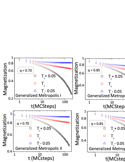
Figure 3: Decay of magnetization according to the power law: $M(t)\sim t^{-\beta/\nu z}$ in the critical temperature found by the considered algorithms (circle red points), for $q=0.70$ and 0.85. We also show the plots considering MC simulations for $T_{c}+\delta$ and $T_{c}-\delta$. It was used $\delta=0.05$. The upper (lower) plots correspond to Metropolis I (II) algorithm.

We use the same procedure to find the critical temperatures for prescription Metropolis II. We find very different results, when compared with that ones obtained with Metropolis I. Similarly to Table 2, we show the results using the Metropolis II prescription in Table 4. The values are smaller than the ones found with Metropolis I prescription. However, they match as $q\rightarrow 1$, which validates the numerical procedure.

$q$	0.70	0.75	0.80	0.85	0.90	0.95	1.00
$k_{B}T_{c}^{(2)}/J$	1.77(1)	1.82(1)	1.89(1)	1.97(1)	2.07(1)	2.17(1)	2.27(1)
$\beta/\nu z$	0.060(4)	0.062(7)	0.078(5)	0.082(2)	0.100(5)	0.094(4)	0.057(3)
$z$	2.13(4)	2.15(5)	2.12(4)	2.09(3)	2.10(3)	2.11(6)	2.15(3)
$\theta$	0.18(4)	0.14(4)	0.22(7)	0.17(3)	0.04(6)	0.17(3)	0.19(4)
$\eta$	0.25(2)	0.27(3)	0.33(2)	0.34(1)	0.42(2)	0.40(2)	0.25(1)
$r$	0.998568758	0.998915473	0.999342437	0.999458152	0.999589675	0.999718708	0.999206853

Table 3: Critical temperature and exponents obtained for different $q$ values for prescription Metropolis I. The exponents where obtained performing simulations for the estimated critical temperatures and were based on power laws previously described in short time regime. The last line we show the $r$ value for the best fits in the second stage (fine scale)

$k_{B}T_{c}^{(1)}/J$	$q=0.70$	$q=0.75$	$q=0.80$	$q=0.85$	$q=0.90$	$q=0.95$	$q=1.00$
$T^{\ast}-0.1$	–	0.369354816	0.393077206	0.473151224	0.555233203	0.664145691	0.754299904
$T^{\ast}=\log(1+\sqrt{2})/2$	–	0.439789081	0.50595381	0.658725599	0.829581264	0.952694449	0.997206853
$T^{\ast}+0.1$	–	0.579484235	0.756653731	0.959530136	0.995694839	0.951627799	0.91284158
$T^{\ast}+0.2$	0.601895662	0.836896384	0.999315534	0.932708995	0.869271327	0.848547425	0.838519074
$T^{\ast}+0.3$	0.844382176	0.989767198	0.875131078	0.833730495	0.831169795	0.799709762	–
$T^{\ast}+0.4$	0.989716381	0.847004746	0.812106454	–	–	–	–
$T^{\ast}+0.5$	0.828738110	0.787203767	–	–	–	–	–
$T^{\ast}+0.6$	0.842827863	–	–	–	–	–	–

Table 4: Coarse grained Stage for Metropolis II - The values of determination coeficient $r$ of the linear fit $\ln\langle M\rangle$ versus $\ln t$, for different $q$ values. As in Table 2, the highest values are in bold correspond to best critical temperature found at first stage (coarse grained).

Similarly, the best results after the fine scale refinement (second stage) are shown in the first line of Table 5.

$q$	0.70	0.75	0.80	0.85	0.90	0.95	1.00
$k_{B}T_{c}^{(2)}/J$	2.66(1)	2.55(1)	2.47(1)	2.41(1)	2.36(1)	2.31(1)	2.27(1)
$\beta/\nu z$	0.019(5)	0.039(5)	0.060(4)	0.094(6)	0.116(7)	0.075(4)	0.057(3)
$z$	1.97(4)	2.02(3)	2.10(3)	2.09(3)	2.09(6)	2.20(4)	2.15(3)
$\theta$	0.43(3)	0.21(7)	0.22(3)	0.11(4)	0.16(5)	0.13(3)	0.19(4)
$\eta$	0.07(2)	0.16(2)	0.25(2)	0.39(3)	0.48(3)	0.33(2)	0.25(1)
$r$	0.994455464	0.998375667	0.999227272	0.999226704	0.99928958	0.99925661	0.997206853

Table 5: Critical temperature and exponents obtained for different $q$ values for the Metropolis II algorithm. The exponents were obtained performing simulations for the estimated critical temperatures. They were based on power laws described in Sec. II. The last line we show the $r$ value for the best fits in the second stage (fine scale)

The magnetization decay obtained by the Metropolis II algorithm depicted in Fig. 3. After obtaining these estimates for the critical temperatures, we perform short time simulations to obtain the critical dynamic exponents $z$ and $\theta$ and the static one $\eta=2\beta/\nu$, using the power laws of Sec. II. Here, we calculated $\theta$ from time correlation $C(t)=\langle M(t)M(0)\rangle$. Tomé and de Oliveira Tania1998 showed that correlation behaves as $C(t)\sim t^{\theta}$, where $\theta$ is exactly the same exponent from initial slope of magnetization from lattices prepared with initial fixed magnetization $m_{0}$. The advantage of this method is that we repeat $N_{s}$ runs, but the lattice does not require a fixed initial magnetization. It is enough to choose the spin with probability 1/2. i.e., $m_{0}=0$ in average. This method does not require the extrapolation $m_{0}\rightarrow 0$.

Figs. 4 and 5 depict plots of time evolving of $F_{2}$ of Eq. 4 and $C(t)$ as a function of $t$ for the different Metropolis algorithm.

To obtain the exponents consider the following steps. Firstly, in simulations that start from the ordered state $m_{0}=1$ and $L=512$, calculate the slope $\beta/\nu z$ of the linear fit of $\ln\langle M(t)\rangle$ as a function of $\ln t$. The error bars are obtained, via running simulations for $N_{bin}=5$, calculating $\langle M(t)\rangle$ that each for seed, with $N_{run}=400$ runs.

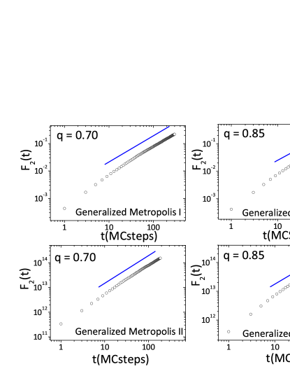
Figure 4: Dynamic cumulant $F_{2}(t)$ versus $t$ in log scale. The slope gives $d/z$ which supplies the $z$-value. Both prescriptions (Metropolis I e II) are studied.

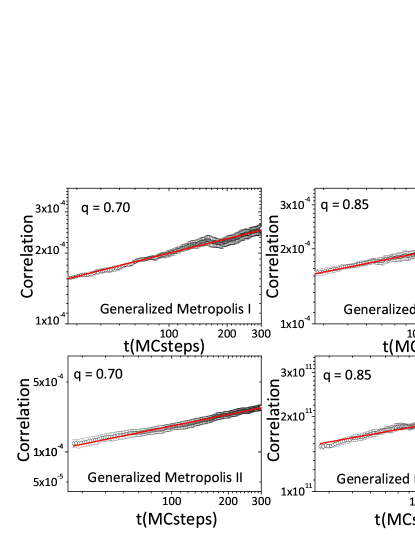
Figure 5: Time correlation of magnetization $C(t)=\left\langle M(t)M(0)\right\rangle$ for two prescriptions: Metropolis I and II.

Once we have calculated $\beta/\nu z$, we estimate $z$ taking the slope in log-log plot $\ln F_{2}$ versus $\ln t$. We used $N_{s}=3000$ different runs starting from random spins configurations with $m_{0}=0$ for time series $\langle M(t)^{2}\rangle$ $\times\ t$ and the same number of runs for time series $\langle M(t)\rangle$ $\times\ t$ starting from $m_{0}=1$(ordered state). Similarly, we repeated the numerical experiment for $N_{bin}=5$ different seeds to obtain the uncertainties. In two dimensional systems, the slope is $\phi=2/z$ (see Eq. 4) and so $z$ is calculated according to $\widehat{z}=2/\widehat{\phi}$ and the uncertainty in $z$ is obtained by relation$\ \sigma_{z}=(2/\phi^{2})\sigma_{\phi}$. Here the $\widehat{\bullet}$ denotes the amount estimated from $N_{bin}=5$ different seeds. Once $z$ is calculated, the exponent $\eta=2\beta/\nu$ is calculated according to $\eta=2\widehat{(\beta/\nu z)}\cdot\widehat{z}$, where $\widehat{(\beta/\nu z)}$ was estimated via magnetization decay and $\widehat{z}$ from cumulant $F_{2}$. The exponent $\theta$ was similarly obtained performing $N_{s}=3000$ different runs to evolve the time series of correlation $C(t)$ and estimating directly the slope in this case.

Tables 3 and 5 show results for the critical exponents obtained with the two algorithms. We do not observe a monotonic behavior of the critical exponents as function of $q$ in either case but on the other hand for both cases we cannot assert, for example, that $z\in[2.09,2.15]$ (Metropolis I) and $z\in[1.97,2.20]\$(Metropolis II) or even other exponents do not change for $q<1$ which implies that we cannot simply extrapolate the critical properties from $q=1$ to $q<1$.

V Conclusions

In the non-extensive thermostatistics context, we have proposed a generalized master equation leading to a generalized Metropolis algorithm. This algorithm is local and satisfies the detailed energy balance to calculate the time evolution of spins systems. We calculate the critical temperatures using the generalized Metropolis dynamics, via equilibrium and non-equilibrium Monte Carlo simulations.

We have obtained the critical parameters performing Monte Carlo simulations in two different ways. Firstly, we show the phase transitions from curves $\left\langle M\right\rangle$ versus $k_{B}T/J$, considering the magnetization averaging, in equilibrium, under different MC steps. Next, we use the short time dynamics, via relaxation of magnetization from samples initially prepared of ordered or disordered states, i.e., time series of magnetization and their moments averaged over initial conditions and over different runs.

We have also studied the Metropolis algorithm of Refs. Crokidakis2009 ; Boer2011 . We show that it does not preserve locality neither the detailed energy balance in equilibrium. While our non-equilibrium simulations corroborate results of Refs.Crokidakis2009 ; Boer2011 when we use their extension of the Metropolis algorithm (Metropolis I), the exponents and critical temperatures obtained are very different when we use our prescription (Metropolis II). When the extensive case is considered, both methods lead to the same expected values.

Simultaneously, we have developed a methodology to refine the determination of the best critical temperature. This procedure is based on optimization of the power laws of the magnetization function that relaxes from ordered state in log scale, via of maximization of determination coefficient of the linear fits. This approach can be extended for other spin systems, since their general usefulness.

For a more complete elucidation about existence of phase transitions for $q\neq 1$, we have performed simulations for small systems MC simulations, recalculating the whole lattice energy in each simple spin flip, according to Metropolis I algorithm only to check the variations on the critical behavior of the model. Notice that this does not apply to Metropolis II algorithm, since it has been designed to work as the standard Metropolis one. Our numerical results show discontinuities in the magnetization, but no finite size scaling, corroborating the results of Ref. Penna1999 , which used the broad histogram technics to show that no phase transition occurs for $q\neq 1$ using Metropolis I algorithm.

It is important to mention that only Metropolis I Crokidakis2009 ; Boer2011 shows inconsistence on critical phenomena of model since global and local simulation schemes leads to different critical properties. Metropolis II overcomes this problem since local and global prescriptions are the same even for $q\neq 1$”. Broad histogram method works with a non-biased random walk that explore the configuration space, leading to a phase transition suppression for $q\neq 1$ Penna1999 . Nevertheless this algorithm must also be adapted to deal with the generalized Boltzmann weight in the same way the master equation needed to be modified. This is out of the scope of the present paper but this issue will be treated in a near future.

References

- (1) C. Tsallis, J. Stat. Phys. 52, 479 (1988).
- (2) C. Tsallis, D. A. Stariolo, Physica. A, 233, 395-406 (1996)
- (3) U. H. E. Hansmann, Physica A 242, 250-257 (1997)
- (4) C. Anteneodo, C. Tsallis and A. S. Martinez, Europhys. Lett. 59, 635-641 (2002).
- (5) N. Destefano and A. S. Martinez, Physica A 390, 1763-1772 (2011).
- (6) A. S. Martinez, R. S. González and C. A. S. Terçariol, Physica A 387, 5679-5687 (2008)
- (7) A. S. Martinez, R. S. González and A. L. Espíndola, Physica A 388, 2922-2930 (2009).
- (8) B. C. T. Cabella, A. S. Martinez and F. Ribeiro, Phys. Rev. E 83, 061902 (2011).
- (9) B. C. T. Cabella, F. Ribeiro and A. S. Martinez, Physica A 391, 1281-1286 (2012).
- (10) R. da Silva, F. Kalil, A. S. Martinez and J. P. M. de Oliveira, Physica A 391, 2119-2128(2012).
- (11) N. Crokidakis, D. O. Soares-Pinto, M. S. Reis, A. M. Souza, R. S. Sarthour, I. S. Oliveira, Phys. Rev. E 80, 051101 (2009).
- (12) A. Boer, Physica A 390, 4203 (2011).
- (13) J. Lima, J. S. Sá Martins, T.J. P. Penna, Physica A 268, 553 (1999)
- (14) B. Zheng, Intr. J. Mod. Phys. B. 12, 1419 (1998)
- (15) H. K. Janssen, B. Schaub, and B. Z. Schmittmann, Phys. B 73, 539 (1989).
- (16) D. A. Huse, Phys. Rev. B 40, 304 (1989).
- (17) E. Arashiro and J. R. Drugowich de Felício, Phys. Rev. E 67, 046123 (2003).
- (18) R. da Silva, N. A. Alves, and J. R. Drugowich de Felício, Phys. Lett. A 298, 325 (2002).
- (19) R. da Silva and J. R. Drugowich de Felício, Phys. Lett. A 333, 277 (2004).
- (20) C. S. Simões and J. R. Drugowich de Felício, Mod. Phys. Lett. B 15, 487 (2001).
- (21) T. Tome, J. R. Drugowich de Felicio, Mod. Phys. Lett. B, 12(21), 873 (1998)
- (22) R. da Silva and N. Alves Jr., Phys. A 350, 263 (2005).
- (23) R. da Silva, R. Dickman, and J. R. Drugowich de Felício, Phys. Rev. E 70, 067701 (2004).
- (24) R. da Silva, N. A. Alves, and J. R. Drugowich de Felício, Phys. Rev. E 66, 026130 (2002).
- (25) H. A. Fernandes, R. da Silva, J. R. Drugowich de Felicio, J. Stat. Mech., P10002 (2006).
- (26) E. Arashiro, J. R. Drugowich de Felício, U. H. E. Hansmann . J. Chem. Phys. 126, 045107 (2007).
- (27) E. Arashiro, J. R. Drugowich de Felício, U. H. E. Hansmann, Phys. Rev. E, vol. 73,(4), 40902 (2006)
- (28) M. L. R. Puzzo, E. V. Albano, Phys. Rev. E, 81 051116 (2010).
- (29) R. Salazar and R. Toral, Phys. Rev. Lett. 83, 4233 (1999).
- (30) C. Tsallis, Química Nova 17, 468 (1994).
- (31) T. J. Arruda, R. S. González, C. A. S. Terçariol and A. S. Martinez, Phys. Lett. A 372, 2578 (2008).
- (32) N. Cressie and T. Read, J. R. Stat. Soc. Ser. B 46, 440 (1984).
- (33) L. Nivanen, A. Le Méhauté and Q.A. Wang, Rep. Math. Phys. 52, 437 (2003).
- (34) E. P. Borges, Physica A 340, 95 (2004).
- (35) M. E. J. Newman, G. T. Barkema, Monte Carlo Method in Statistical Physics, Oxford (1999)
- (36) T. Tomé and M. J. de Oliveira, Phys. Rev. E. 58, 4242 (1998).