Refined Checks and Exact Dualities
in Three Dimensions

Abstract

We discuss and provide nontrivial evidence for a large class of dualities in three-dimensional field theories with different gauge groups. We match the full partition functions of the dual phases for any value of the couplings to underpin our proposals. We focus on two classes of models. The first class, motivated by the AdS/CFT conjecture, consists of necklace $U(N)$ quiver gauge theories with non chiral matter fields. We also consider orientifold projections and establish dualities among necklace quivers with alternating orthogonal and symplectic groups. The second class consists of theories with tensor matter fields with free theory duals. In most of these cases the $R$-symmetry mixes with IR accidental symmetries and we develop the prescription to include their contribution into the partition function and the extremization problem accordingly.

1 Introduction

Three dimensional dualities between supersymmetric field theories have been studied since a long time. Some of them are similar to the four dimensional case of Seiberg duality, like the Aharony duality Aharony:1997gp and the Giveon-Kutasov one Giveon:2008zn .

More recently, new nonperturbative techniques have been used to gain more insights into aspects of three-dimensional field theories. In particular, the exact partition function of any ${\cal N}\geq 2$ superconformal field theory reduces to a matrix model for any value of the coupling constants Kapustin:2009kz ; Jafferis:2010un ; Hama:2010av , and gives information about physical quantities of the given model Suyama:2009pd ; Herzog:2010hf ; Martelli:2011qj ; Cheon:2011vi ; Jafferis:2011zi ; Amariti:2011uw ; Minwalla:2011ma ; Amariti:2011da ; Amariti:2011jp ; Gang:2011jj ; Amariti:2011xp ; Drukker:2010nc ; Amariti:2012tj that can be compared with previous results Bagger:2006sk ; Bagger:2007jr ; Gustavsson:2007vu ; Bagger:2007vi ; Aharony:2008ug ; Gaiotto:2007qi ; Avdeev:1992jt ; Jafferis:2008qz ; Martelli:2008si ; Hanany:2008cd ; Hanany:2008fj ; Ueda:2008hx ; Imamura:2008nn ; Franco:2008um ; Hanany:2008gx ; Bianchi:2009ja ; Amariti:2009rb ; Franco:2009sp ; Bianchi:2009rf ; Davey:2009sr .

Moreover, one can also compare the partition functions of two field theories that are conjectured to describe dual phases of the same superconformal fixed point, thus providing a nontrivial check of the duality. Showing that both sides share the same partition function is non trivial . One can consider different limits. Seiberg-like dualities for theories with at least ${\cal N}=3$ supersymmetry have been considered in Kapustin:2010mh ; Kapustin:2010xq . With lower supersymmetry, the partition function is considerably more complicated. In the large-$N$ limit, one can use the saddle point approximation and successfully study infinite classes of theories which involve an arbitrary product gauge group Amariti:2011uw ; Gulotta:2011vp . For finite values of the gauge group rank and Chern-Simons (CS) level one can exploit the following observation. Exact results can be also obtained by generalizing the three-dimensional space on which the theory is defined to a squashed three-sphere, which enjoys a $U(1)^{2}$ subgroup of the isometry group $SU(2)^{2}$ of $S^{3}$. The localized partition function on this space can be written in terms of hyperbolic functions Hama:2011ea . A review of their properties is given in fvdb , and in appendix A, and they have revealed themselves very useful to give further evidence to a large class of dualities Willett:2011gp ; Kapustin:2011gh ; Benini:2011mf ; Niarchos:2012ah .

In most of these cases a single gauge group has been considered, but in principle one can use the same approach to match exact results for physical quantities among dual phases of theories describing generic configurations of M$2$ branes.

In this paper we are interested in different classes of dualities. Some of these have been considered in the framework of the large-$N$ approximation of the partition function in Amariti:2011uw ; Gulotta:2011vp . However, this limit does not catch an important subtlety of the duality transformation. If one starts with a product of unitary gauge groups $\prod U(N)_{k_{i}}$ in the electric theory and performs a duality transformation on the group $i$ the resulting dual gauge group contains a factor $U(N+|k_{i}|)$. At the leading order in a large-$N$ expansion, this dependence upon the CS level $k$ does not play any role. We drop the large-$N$ limit and provide nontrivial evidence for this duality to hold at any value of $N$ and the $k$’s in section 4. We also consider other models, which can be derived as the low energy theories living on the worldvolume of intersecting D-branes and orientifold O-planes, their dual phases and match the finite-$N$ partition function for them.

Another interesting set of dualities recently proposed in Jafferis:2011ns and extended in Kapustin:2011vz can be studied by computing the partition function on the squashed three-sphere. In these cases we re-derive some of the known results by applying the exact calculations of fvdb and we compare with known dualities.

In these cases one has to pay attention to infrared accidental symmetries. Indeed in some cases the exact computation shows that some theories look dual to free theories in which the scaling dimensions of the gauge invariant operators are not consistent with the free theory value. A proper modification of the extremization principle, to account for the mixing of accidental symmetries with the $R$-symmetry, is necessary for the calculation of the exact $R$-charge.

The paper is organized as follows. In section 2 we review the rules to write the all-loop partition function on a squashed three-sphere, and show how it can be written in terms of hyperbolic functions. We also list a few basic properties of the hyperbolic functions. In section 3 we review some of the classes of models we are interested in. We describe how they can be embedded in a type IIB setup, and how the duality transformations follow from this embedding. We consider theories with unitary, orthogonal and symplectic factors in the product gauge group. The dualities are proved for any value of the ranks and CS levels in section 4 through the matching of the partition functions on both sides. Models with free field theory duals will be considered in section 5, where we also raise the problem of accidental symmetries which we further describe in section 6. Open problems and hints for future work are discussed in section 7. We include some appendices which contain technical details.

2 The partition function on a squashed three sphere

Localization has allowed to reduce the partition function of any $\mathcal{N}=2$ three dimensional supersymmetric theory on a three sphere $S^{3}$ Jafferis:2010un ; Hama:2010av . A further refinement Hama:2011ea involves two different squashed spheres $S_{b}^{3}$: One of them preserves an $SU(2)\times U(1)$ isometry, but in this case the localization does not give any new result, the other one, which will be very useful in this paper, preserves an $U(1)^{2}$ isometry. The partition function on the latter squashed sphere $S_{b}^{3}$ for a CS matter theory with gauge group $G$ is

$$\mathcal{Z}_{S_{b}^{3}} = \int_{\mathbb{T}^{\text{rk}(G)}}\prod_{i=1}^{\text{rk}(G)}dx_{i}e^{i\pi kTr_{F}x^{2}}\det_{~{}~{}~{}~{}adj}\left(\sinh\left(\pi b\rho_{\alpha}(x)\right)\sinh\left(\pi b^{-1}\rho_{\alpha}(x)\right)\right)$$ (1)

$$\times \prod_{\rho\in r}S_{b}\left(\frac{i}{2}(b+b^{-1})(1-\Delta_{r})-\rho_{r}(x)\right)$$

where $\Delta_{r}$ is the scaling dimension (which in three dimensions coincides with the $R$-charge) of a chiral matter field in the representation $r$, $\rho_{r}$ are the weights of the representation $r$, and $\rho_{\alpha}$ are the roots of the gauge groups $G$. The various factors in the integrand in (1) correspond to the contribution from the CS term, the vector multiplet and the matter superfields (in the representation $r$) respectively. The function $S_{b}$ is the double sine function defined as

$$S_{b}\left(\frac{i}{2}(b+b^{-1})(1-\Delta_{r})-\rho(x)\right)=\prod_{n_{1},n_{2}\geq 0}^{\infty}\frac{n_{1}b+n_{2}b^{-1}+\frac{b+b^{-1}}{2}+i\rho(x)+\frac{b+b^{-1}}{2}(1-\Delta_{r})}{n_{1}b+n_{2}b^{-1}+\frac{b+b^{-1}}{2}-i\rho(x)-\frac{b+b^{-1}}{2}(1-\Delta_{r})}$$ (2)

The limit $b=1$ corresponds to the round sphere considered in Jafferis:2010un ; Hama:2010av . In that case the double sine reduces to

$$S_{1}\left(i(1-\Delta_{r})-\rho(x)\right)\equiv S_{1}(iz)=e^{l(z)}$$ (3)

where $l(z)$ is defined such that its derivative is $-\pi z\cot(\pi z)$.

The partition function on the squashed sphere is more complicated than the corresponding one on the round sphere. However, since the double sine function can be identified with the hyperbolic Gamma function Ruijsenaars , we can exploit the recent work by mathematicians which provide us with exact results for the integral involved in physical computations fvdb . In the following we introduce the basic definitions relevant for this paper, and provide more technical details to appendix A.

2.1 Hyperbolic functions

We start by introducing the periods $\omega_{1}$ and $\omega_{2}$, that in this case are identified with

$$\omega_{1}=ib\quad,\quad\omega_{2}=ib^{-1}\quad,\quad\omega=\frac{\omega_{1}+\omega_{2}}{2}$$ (4)

The double sine function in terms of $\omega_{1}$, $\omega_{2}$ and $z$ becomes

$$S(-iz;-i\omega_{1},-i\omega_{2})=\prod_{n1,n2\geq 0}^{\infty}\frac{(n_{1}+1)\omega_{1}+(n_{2}+1)\omega_{2}-z}{n_{1}\omega_{1}+n_{2}\omega_{2}+z}$$ (5)

This corresponds to the hyperbolic gamma function $\Gamma_{h}(z;\omega_{1},\omega_{2})\equiv\Gamma_{h}(z)$ first defined in Ruijsenaars . This function satisfies the difference equations

$$\Gamma_{h}(z+\omega_{1})=2\sin\left(\frac{\pi z}{\omega_{2}}\right)\Gamma_{h}(z)\quad,\quad\Gamma_{h}(z+\omega_{2})=2\sin\left(\frac{\pi z}{\omega_{1}}\right)\Gamma_{h}(z)$$ (6)

and the reflection formula

$$\Gamma_{h}(z+\psi_{1})\Gamma_{h}(\psi_{2}-z)=1\quad\quad\text{if}\quad\quad\psi_{1}+\psi_{2}=2\omega$$ (7)

Other useful identities are

$$\Gamma_{h}(\omega)=1\,,\,\Gamma_{h}\left(\frac{\omega_{1}}{2}\right)=\Gamma_{h}\left(\frac{\omega_{2}}{2}\right)=\frac{1}{\sqrt{2}}\,,\,\Gamma_{h}\left(\omega+\frac{\omega_{1}}{2}\right)=\Gamma_{h}\left(\omega+\frac{\omega_{2}}{2}\right)=\sqrt{2}$$ (8)

and

$$\Gamma_{h}(2z)=\Gamma_{h}\left(z\right)\Gamma_{h}\left(z+\frac{\omega_{1}}{2}\right)\Gamma_{h}\left(z+\frac{\omega_{2}}{2}\right)\Gamma_{h}(z+\omega)$$ (9)

By combining (6) and (7) one has

$$\Gamma_{h}(\pm z)\equiv\Gamma_{h}(z)\Gamma_{h}(-z)=\frac{\Gamma_{h}(z+\omega_{1})\Gamma_{h}(\omega_{2}-z)}{4\sin\left(\frac{\pi z}{\omega_{1}}\right)\sin\left(-\frac{\pi z}{\omega_{2}}\right)}=-\frac{1}{4\sin\left(\frac{\pi z}{\omega_{1}}\right)\sin\left(\frac{\pi z}{\omega_{2}}\right)}$$ (11)

which correspfonds to the one loop contribution of the vector multiplet in (1). The final expression for the partition function in terms of the hyperbolic gamma function is

$$\mathcal{Z}(\Delta_{R},\omega_{1},\omega_{2})=\frac{1}{\sqrt{(-\omega_{1}\omega_{2})^{n}}{\cal W}}\int\prod_{i=1}^{n}du_{i}e^{\frac{-i\pi k}{\omega_{1}\omega_{2}}x_{i}^{2}}\frac{\prod_{\rho_{r}\in R}\Gamma_{h}(\rho_{r}(x)+\omega\Delta_{R})}{\prod_{\rho_{\alpha}\in\alpha^{(+)}}\Gamma_{h}(\pm\rho_{\alpha}(x_{i}))}$$ (12)

where $\cal W$ is the dimension of the Weyl subgroup and $n$ is the rank of the gauge group. Many exact results concerning these integrals have been studied in fvdb . To deal with the notations there we define the functions $c(x)$ and $\zeta$ as

$$c(x)\equiv\exp\left(\frac{i\pi x}{2\omega_{1}\omega_{2}}\right)\quad,\quad\zeta=e^{\frac{i\pi(\omega_{1}^{2}+\omega_{2}^{2})}{24\omega_{1}\omega_{2}}}$$ (13)

in terms of which the CS contribution at level $k=-\frac{t}{2}$ is

$$\exp\left({\frac{i\pi t}{2\omega_{1}\omega_{2}}x_{i}^{2}}\right)=c(tx_{i}^{2})$$ (14)

Also notice that in the $S^{3}$ limit, $\omega_{1}=\omega_{2}=i$, we obtain $\log\left(\Gamma_{h}\left(z\right)\right)=l(1+iz)$ which is the one loop contribution of matter fields computed in Jafferis:2010un .

3 Families of quiver gauge theories and M$2$ branes

In this section we survey the classes of models dual to M$2$ branes on Calabi-Yau fourfold that we will be interested in. These models have been deeply investigated in Jafferis:2008qz ; Martelli:2008si ; Hanany:2008cd ; Hanany:2008fj ; Ueda:2008hx ; Imamura:2008nn ; Franco:2008um ; Hanany:2008gx ; Amariti:2009rb ; Franco:2009sp ; Davey:2009sr .

Each one can be understood in the framework of type IIB SUGRA compactified on a circle. The low energy brane dynamics is described by the worldvolume theory living in the $2+1$ infinite directions of some D$3$ brane suspended between pairs of $(1,p_{i})$ fivebranes. The latter picture also provides us with a representation in terms of quiver diagrams, according to which we associate a node to each gauge group and an arrow to each matter field. We distinguish two types of arrows: one which connects two distinct nodes is associated to bifundamental matter fields, while one that has both its endpoints on the same node represents a chiral field in the adjoint representation.

In the three-dimensional case, in addition to the above information we also have to provide the CS levels. In the type IIB picture, they are given by the difference $(p_{i}-p_{i-1})$. From a purely field theoretical point of view, our only constraint will be that they add up to zero.

Finally, we will let the gauge group factors to be either the unitary, orthogonal or symplectic group (i.e. we also consider cases with O$3$ planes in the brane construction).

3.1 Unitary groups

We take type IIB string theory compactified on a circle, which we parametrize with the $x_{6}$ coordinate. The worldvolume theory of a stack of $N$ D$3$ branes wrapped on the circle is described by a $U(N)$ gauge theory in three dimensions. If the D$3$’s intersect $g$ NS$5$ extended along the D$3$ worldvolume but not around the circle, the gauge group contains $g$ $U(N)$ factors. The introduction of the CS terms is achieved by replacing the NS$5$ with a tilted bound state of NS$5$ and $p_{i}$ D$5$, dubbed $(1,p_{i})$ fivebrane. We refer to table 1 for the precise definition of the embedding. The $(0,1,2)$ directions represent the three-dimensional spacetime, with $x_{6}$ compact.

brane	0	1	2	3	4	5	6	7	8	9
D$3$	X	X	X				X
NS$5_{\alpha}$	X	X	X	X	X	X
NS$5_{\beta}$	X	X	X	X					X	X
D$5_{\alpha}$	X	X	X		X	X		X
D$5_{\beta}$	X	X	X					X	X	X

Table 1: Type IIB embedding of low energy CS field theories.

The $\alpha$-th NS$5$ brane, $\alpha=1,\ldots,a$, combines with the $Q_{\alpha}$ D$5_{\alpha}$ branes to give a $(1,Q_{\alpha})$-fivebrane stretched along the $012[37]_{\theta_{\alpha}}45$ direction. The $\beta$-th NS$5$ brane, $\beta=1,\ldots,b$, combines with the $P_{\beta}$ D$5_{\beta}$ branes to give a $(1,P_{\beta})$-fivebrane stretched along the $012[37]_{\theta_{\beta}}89$ direction. For specific values of the angles $\theta_{\alpha}$ and $\theta_{\beta}$ determined by $Q_{\alpha}$ and $P_{\beta}$, the supersymmetry is enhanced to ${\cal N}\geq 3$. We will consider generic configurations, so our results will be also valid when this enhancement does occur. The fivebranes are chosen to be placed in the following order: first we put $b-a$ $(1,P_{\beta})$ fivebranes on the circle and then we alternate the remaining $a$ $(1,P_{\beta})$ and the $a$ $(1,Q_{\alpha})$.

The $N_{i}$ D$3$-branes stretched between each pair of $(1,p_{i})$ give rise to a $U(N_{i})_{k_{i}}$ gauge group in the quiver. Each $(1,p_{i})$ is associated to a pair of bifundamental chiral fields in the $(N_{i},\bar{N}_{i+1})$ representation. In addition, we have an adjoint chiral field for each consecutive pair of $(1,p_{i})$ of the same type. The resulting field theory is a $\prod_{i=1}^{g}U(N_{i})_{k_{i}}$ gauge theory, where $k_{i}$ represents the CS level of the $i$-th group and $g=b+a$. The levels are given by the relation $k_{i}=p_{i}-p_{i+1}$ which also implies $\sum k_{i}=0$. In the quiver representation we have the first $b$ nodes with adjoint matter and the last $a$ without adjoints; every pair of consecutive nodes is connected by a pair of bifundamental and anti-bifundamental fields. We also obtain the following superpotential

$$W=X_{1,1}X_{1,a+b}X_{a+b,1}+\sum_{i=1}^{b-a}X_{i,i}X_{i,i+1}X_{i+1,i}+\sum_{i=b-a+1}^{a+b}X_{i,i-1}X_{i-1,i}X_{i,i+1}X_{i+1,i}$$ (15)

where $X_{i,j}$ indicates a bifundamental field connecting nodes $i$ and $j$ and $X_{i,i}$ corresponds to an adjoint of the node $i$. Globally, the brane construction and thus the field theory preserves $\mathcal{N}=2$ supersymmetry.

3.1.1 Duality

The above brane picture allows us to describe Seiberg-like dualities in an unified way, through the Hanany-Witten transition Hanany:1996ie . Consider two consecutive, non-parallel, $(1,p_{i})$ fivebranes and move one towards the other until they cross and exchange their positions along the $x_{6}$ direction. Quantum charge conservation requires the creation of $|P_{\beta_{b+i}}-Q_{\alpha_{i}}|=k_{b+i}\,\,$ D$3$ branes on top of the existing $N_{b+i}$ ones.

Correspondingly, in the low energy field theory the $i$-th gauge factor changes its rank from $N_{i}$ to $N_{i}+|k_{i}|$, and because the fivebrane charges and order determine the CS levels, the latter also undergo the following shift

$$k_{i-1} = p_{i-1}-p_{i}\,\,\to\,\,k_{i-1}^{\prime}=p_{i-1}-p_{i+1}=k_{i-1}+k_{i}$$

$$k_{i} = p_{i}-p_{i+1}\,\,\to\,\,k_{i}^{\prime}=p_{i+1}-p_{i}=-k_{i}$$ (16)

$$k_{i+1} = p_{i+1}-p_{i+2}\,\,\to\,\,k_{i+1}^{\prime}=p_{i}-p_{i+2}=k_{i+1}+k_{i}$$

Note that the sum of all the CS levels is preserved in this process. The local nature of the Hanany-Witten transition is reflected in the field theory by the fact that only one gauge group and its first neighbors go through a change. Finally the superpotential locally changes as

$$\widetilde{W} = Y_{b+i-1,b+i-1}Y_{b+i-1,b+i}Y_{b+i,b+i-1}+Y_{b+i,b+i-1}Y_{b+i-1,b+i}Y_{b+i,b+i+1}Y_{b+i+1,b+i}$$ (17)

$$+ Y_{b+i+1,b+i+1}Y_{b+i+1,b+i}Y_{b+i,b+i+1}$$

Notice that the dual theory also contains two new adjoint fields. Thanks to the above superpotential, the two models have the same moduli space and are conjectured to be dual to each other in the deep infrared. Also notice that nowhere did we use the fact that in this example the electric ranks of the gauge groups are equal to each other. Thus the same argument can be straightforwardly applied to a product of arbitrary unitary groups.

The duality above extends the Kutasov-Giveon duality Giveon:2008zn for three dimensional supersymmetric gauge theories with CS terms. Nontrivial checks are required in order to validate the whole picture provided above. In fact, there exist two limits where such checks have been given. One is the large $N$ limit Amariti:2011uw . In this case, the dual gauge group can be safely taken to be the original one, because any difference in the ranks due to the CS levels is subleading. Notice that, in general, this is a nontrivial statement.

The second limit corresponds to the case of finite $N$ with $\mathcal{N}\geq 3$. Only partial results have been studied in this limit. For instance, when $a=b=1$ the model is the ABJM model which enjoys $\mathcal{N}=6$ supersymmetry. In that case the analysis becomes much simpler and many checks have been provided. In fact, beside the moduli space matching, there is no check for models with $g>2$ gauge group factors and ${\cal N}=2$ supersymmetry. The main difficulties in this case are due to the nontrivial anomalous dimensions of the fields. We will see how we can identify the scaling dimensions of the fields on the two sides of the duality so that the two partition functions agree even for $g>2$ and for arbitrary ranks. We will also argue that the map we will describe preserves extremization of the partition function with respect to scaling dimensions themselves.

3.2 Orthogonal and symplectic groups: the orientifold

While we focused on unitary gauge groups in the above subsection, more general models can be derived from the same type IIB picture above. An immediate extension includes adding orientifold O$3$ planes on top of the D$3$ branes, which we employ in the following. This construction does not break any residual supersymmetry, so we will end up with ${\cal N}\geq 2$ theories Hosomichi:2008jb ; Aharony:2008gk .

For simplicity, we restrict to the class of theories with $a=b$. Under the orientifold projection, the $(1,p_{i})$ fivebranes which intersect the O$3$ are identified with their own image while the projection does not act on the D$3$ branes. There are four kind of O$3$ planes, named O$3^{\pm}$ and $\widetilde{O3}^{\pm}$, that differ, among other, by the amount of D$3$ brane charge they carry, and by the resulting worldvolume theory gauge group they lead to. We summarize the different cases in table 2.

Type	Charge	Group
O$3^{+}$	$\,-\frac{1}{4}$	$SP(2N)$
O$3^{-}$	$~{}~{}~{}\frac{1}{4}$	$SO(2N)$
$\widetilde{\text{O}3}^{+}$	$~{}~{}~{}\frac{1}{4}$	$SP(2N)$
$\widetilde{\text{O}3}^{-}$	$~{}~{}~{}\frac{1}{4}$	$SO(2N+1)$

Table 2: O$3$ planes, their D$3$ brane charge and the corresponding gauge group.

A $(1,p_{i})$ fivebrane which intersects the orientifold plane switches its type according to the following rule: If $p_{i}$ is even we have $(\text{O}3^{+},\widetilde{\text{O}3}^{+})\leftrightarrow(\text{O}3^{-},\widetilde{\text{O}3}^{-})$ otherwise if $p_{i}$ is odd we have $(\text{O}3^{\pm}\leftrightarrow\widetilde{\text{O}3}^{\mp})$. We restrict to the case of $p_{i}$ even and make this explicit by considering $(1,2p_{i})$ instead. According to the general discussion on the brane engineering of CS matter theories above, all the CS terms will be even too.

It is then clear that the gauge group will include alternating factors of orthogonal and symplectic groups. Their ranks are given by the choice of the O$3$ planes, namely we obtain a chain of $SO(2N)_{2k_{i}}\times SP(2N)_{k_{j}}$ factors for alternating O$3^{+}$ and O$3^{-}$ planes, and of $SO(2N+1)_{2k_{i}}\times SP(2N)_{k_{j}}$ factors in the $\widetilde{\text{O}3}^{\pm}$ case (with the convention $SP(2)\simeq SU(2)$). An example of such construction is given in figure 1 for the case with O$3^{\pm}$.

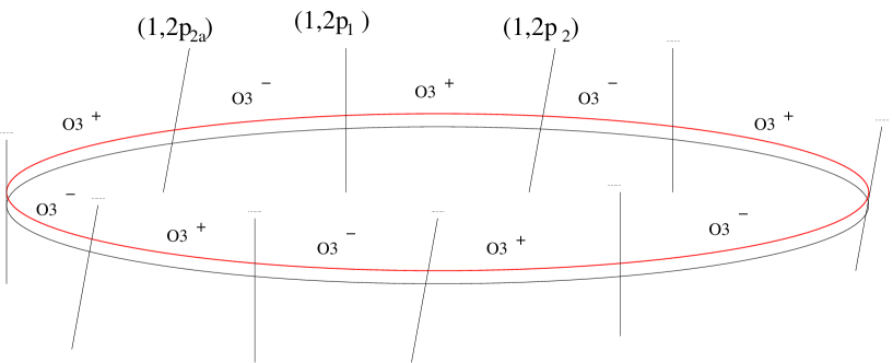
Figure 1: A type IIB embedding of orthogonal and symplectic field theories via O$3^{\pm}$ planes on a stack of D$3$.

The fields are projected such that every pair of bifundamental and anti-bifundamental becomes a single field in the fundamental of both the $SP$ and $SO$ node. By starting with $X_{i-1,i}$ and $X_{i,i-1}$ one ends up with a single field $X_{i-1,i}$ when we fix the left to right convention on the indices. The superpotential is

$$W=\left(X_{i-1,i}\cdot X_{i,i+1}\right)^{2}$$ (18)

where the products are appropriately taken in the $SP$ and/or $SO$ case.

3.2.1 Duality

We again apply the brane creation effect when two fivebranes cross each other to derive the rules for the low energy field theory duality. The steps are in close analogy with the ones above, with the charge of the O$3$ plane properly taken into account.

Because the duality only acts locally on the quiver, we can isolate the node over which we perform the fivebrane exchange and collect the changes in the gauge group and CS level of itself and its neighbors as follows: suppose we apply the duality on the node $A$ which locally looks like

A-1	A	A+1
$SO(2N)_{2k_{A-1}}$	$SP(2N)_{k_{A}}$	$SO(2N)_{2k_{A+1}}$
$SO(2N+1)_{2k_{A-1}}$	$SP(2N)_{k_{A}}$	$SO(2N+1)_{2k_{A+1}}$
$SP(2N)_{k_{A-1}}$	$SO(2N)_{2k_{A}}$	$SP(2N)_{k_{A+1}}$
$SP(2N)_{k_{A-1}}$	$SO(2N+1)_{2k_{A}}$	$SP(2N)_{k_{A+1}}$

with superpotential (18). Then the dual theory is locally given by

A-1	A	A+1
$SO(2N)_{2k_{A-1}+2k_{A}}$	$SP(2(N+|k_{A}|-1)_{-k_{A}}$	$SO(2N)_{2k_{A+1}+2k_{A}}$
$SO(2N+1)_{2k_{A-1}+2k_{A}}$	$SP(2(N+|k_{A}|-1))_{-k_{A}}$	$SO(2N+1)_{2k_{A+1}+2k_{A}}$
$SP(2N)_{k_{A-1}+k_{A}}$	$SO(2(N+k_{A}-1))_{-2k_{A}}$	$SP(2N)_{k_{A+1}+k_{A}}$
$SP(2N)_{k_{A-1}+k_{A}}$	$SO(2(N+|k_{A}|)+1)_{-k_{A}}$	$SP(2N)_{k_{A+1}+k_{A}}$

with all the remaining nodes in the quiver unchanged and dual superpotential given by

$$\tilde{W}=Y_{A-1,A-1}\cdot Y_{A-1,A}^{2}+Y_{A-1,A}^{2}Y_{A,A+1}^{2}+Y_{A+1,A+1}\cdot Y_{A+1,A}^{2}$$ (19)

These dualities fit with the ones proposed in Kapustin:2011gh for the case without the quiver structure, and with the ones for the case of two gauge groups and higher supersymmetry Aharony:2008gk .

In the following we will show that the partition function is preserved at finite $N$ for all of these dualities.

4 Exact results for the dualities

In this section we evaluate the exact partition function on a squashed three sphere of the above models and provide further evidence for the dualities. We review the identities we use in Appendix A and also refer to fvdb for more details. Because the duality only acts on the local structure of the quiver, we can restrict ourselves to the the subset of variables which undergo the duality transformation. In other words, we explicitly write only the integration variables corresponding to the gauge group factor we are performing the duality on.

4.1 Duality in $U(N)_{k}$ non-chiral quivers

In this case the large $N$ partition function have been studied in Drukker:2010nc ; Herzog:2010hf ; Martelli:2011qj ; Jafferis:2011zi ; Cheon:2011vi ; Suyama:2009pd ; Amariti:2011uw , and the agreement between dual phases have been checked in this limit in Kapustin:2010mh ; Kapustin:2010xq ; Gulotta:2011vp ; Amariti:2011uw ; Amariti:2012tj . Here we provide the agreement at finite $N$.

In terms of the hyperbolic functions defined in section 2, the partition function for models with only unitary gauge groups can be written in a very compact way. The matter content and local quiver structure are represented in figure 2, where we used the letter $A$ to label the gauge group factor over which we perform the duality. From the top figure we read the relevant contribution to the partition function involved in the duality as

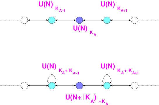
Figure 2: Dual phases describing a stack of M$2$ branes probing a Calabi-Yau fourfold.

$$\mathcal{Z}_{e} = \frac{1}{\sqrt{\left(-\omega_{1}\omega_{2}\right)^{N}}N!}\displaystyle\int\!\frac{\displaystyle\prod_{J=A-1}^{A}\prod_{i,j=1}^{N}\prod_{\eta=\pm 1}\Gamma_{h}\left(\eta\left(x_{J}^{(i)}-x_{J+1}^{(j)}\right)+\omega\Delta_{J,J+1}^{(\eta)}\right)}{\displaystyle\prod_{i<j}^{N}\Gamma_{h}\left(\pm\left(x_{A}^{(i)}-x_{A}^{(j)}\right)\right)}$$ (20)

$$\times \prod_{J=A-1}^{A+1}\prod_{i=1}^{N}c\left(-2k_{J}{x_{J}^{(i)}}^{2}\right)\prod_{i=1}^{N}dx_{A}^{(i)}$$

where the round sphere corresponds to the limit $\omega_{1}=\omega_{2}=\omega=i$. Our aim is to write (20) in a form that can be interpreted as the partition function of the dual theory described in section 3. We find it is useful to define the following shorthand notation

$$\begin{array}[t]{cc}\begin{array}[]{l}\Delta_{J,J+1}=\Delta_{J,J+1}^{(+)}\\ \mu_{A+1}^{(i)}=x_{A+1}^{(i)}+\omega\Delta_{A,A+1}^{(-)}\\ \nu_{A+1}^{(i)}=-x_{A+1}^{(i)}+\omega\Delta_{A,A+1}^{(+)}\\ \mu_{r}=\{\mu_{A-1}^{(i)},\mu_{A+1}^{(i)}\}\end{array}&\qquad\,\,\begin{array}[]{l}\Delta_{J+1,J}=\Delta_{J,J+1}^{(-)}\\ \mu_{A-1}^{(i)}=x_{A-1}^{(i)}+\omega\Delta_{A-1,A}^{(+)}\\ \nu_{A-1}^{(i)}=-x_{A-1}^{(i)}+\omega\Delta_{A-1,A}^{(-)}\\ \nu_{s}=\{\nu_{A-1}^{(i)},\nu_{A+1}^{(i)}\}\end{array}\end{array}$$ (30)

which satisfy the superpotential contraint

$$\sum_{r=1}^{2N}\mu_{r}+\sum_{s=1}^{2N}\nu_{s}=N\omega(\Delta_{A,A+1}^{(-)}+\Delta_{A,A+1}^{(+)}+\Delta_{A-1,A}^{(-)}+\Delta_{A-1,A}^{(+)})=2\omega N$$ (31)

Here $r$ and $s$ are collective indices for elements of the respective sets. By applying equation (98) and fixing $k_{A}>0$ we obtain

$$\mathcal{Z}_{m} = \frac{1}{\sqrt{(-\omega_{1}\omega_{2})^{N+k_{A}}}(N+k_{A})!}\int\frac{\displaystyle\prod_{J=A\pm 1}\prod_{i=1}^{N}\prod_{j=1}^{N+k_{A}}\Gamma_{h}\left(\omega-\nu_{J}^{(i)}-x_{A}^{(j)}\right)\,\Gamma_{h}\left(\omega-\mu_{J}^{(i)}+x_{A}^{(j)}\right)}{\displaystyle\prod_{i<j}^{N+k_{A}}\Gamma_{h}\left(\pm\left(x_{A}^{(i)}-x_{A}^{(j)}\right)\right)}$$ (32)

$$\prod_{i=1}^{N}c\left(-2(k_{A}+k_{J}){x_{J}^{(i)}}^{2}\right)\prod_{i=1}^{N+k_{A}}c\left(2k_{A}{x_{A}^{(i)}}^{2}\right)dx_{A}^{(i)}\times\prod_{r,s=1}^{2N}\Gamma_{h}\left(\mu_{r}+\nu_{s}\right)$$

$$\zeta^{-k_{A}^{2}-2}\,\,c\left(k_{A}^{2}\left(2\omega^{2}-1\right)+2\,N\,k_{A}\left(\omega^{2}\left(\Delta_{A-1,A}^{2}+\Delta_{A,A+1}^{2}-2\right)-1\right)\right)$$

The denominator can be interpreted as the 1-loop contribution from the vector superfield of the gauge group $U(N+k_{A})$ (recall that the duality does not change the ranks of other factors). The numerator in the first term contains the contribution from the (anti)bifundamental fields: it is easy to see that bifundamental fields are mapped to anti-bifundamental fields and viceversa, as required by Seiberg duality. Moreover, we also obtain the offshell map between the scaling dimensions $\tilde{\Delta}$ of the dual fields and the electric ones

$$\widetilde{\Delta}_{A,A\pm 1}=1-\Delta_{A\pm 1,A}\qquad\qquad\widetilde{\Delta}_{A\pm 1,A}=1-\Delta_{A,A\pm 1}$$ (33)

The last factor in the second line of (32) gives the contribution from the new adjoint fields. Indeed, it can be written in the form

$$\prod_{r,s=1}^{2N}\Gamma_{h}(\mu_{r}+\nu_{s}) = \prod_{J=A\pm 1}\prod_{i,j=1}^{N}\Gamma_{h}\left(x_{J}^{(i)}-x_{J}^{(j)}+\omega\widetilde{\Delta}_{J,J}\right)\times$$ (34)

$$\prod_{i,j=1}^{N}\Gamma_{h}\left(x_{A+1}^{(i)}-x_{A-1}^{(j)}+\omega(\Delta_{A,A+1}^{(+)}+\Delta_{A-1,A}^{(-)})\right)$$

$$\prod_{i,j=1}^{N}\Gamma_{h}\left(x_{A-1}^{(i)}-x_{A+1}^{(j)}+\omega(\Delta_{A,A+1}^{(-)}+\Delta_{A-1,A}^{(+)})\right)$$

where $\widetilde{\Delta}_{A\pm 1,A\pm 1}=\Delta_{A\pm 1,A}+\Delta_{A,A\pm 1}$ gives the $R$-charge of the adjoint fields. On the field theory side the dual superpotential is

$$W=\dots + Y_{A,A-1}Y_{A-1,A-1}Y_{A-1,A}+Y_{A-1,A}Y_{A,A+1}Y_{A+1,A-1}$$ (35)

$$+ Y_{A+1,A}Y_{A,A-1}Y_{A-1,A+1}+Y_{A,A+1}Y_{A+1,A+1}Y_{A+1,A}+\dots$$

and by integrating out the fields $Y_{A-1,A+1}$ and $Y_{A+1,A-1}$ it becomes

$$W=Y_{A,A-1}Y_{A-1,A-1}Y_{A-1,A}-Y_{A-1,A}Y_{A,A+1}Y_{A+1,A}Y_{A,A-1}+Y_{A,A+1}Y_{A+1,A+1}Y_{A+1,A}+\dots$$

where the dual fields $Y_{A\pm 1,A\pm 1}$ are related to the electric ones as

$$Y_{A\pm 1,A\pm 1}=X_{A\pm 1,A}X_{A,A\pm 1}$$ (37)

Formula (34) takes properly into account the contribution of the new mesons $Y_{A+1,A+1}$ and $Y_{A-1,A-1}$. The contribution of the two extra mesons reduces to $1$ in (34) after using the reflection formula (7) and the superpotential constraint$\widetilde{\Delta}_{A-1,A+1}+\widetilde{\Delta}_{A+1,A-1}=2$.

We now check that the CS levels shift according to the discussion in section 3. For simplicity we gauge fix the complexified Fayet-Iliopoulos (FI) term $\Delta_{m}$ to zero, but the corresponding generalization is straightforward and one can easily map the electric FI in the magnetic one as $\Delta_{m}^{\prime}$ = $\Delta_{m}^{\prime}\left(\Delta_{m},\Delta_{J,J+1}^{(\pm)}\right)$. We stress that we can perform this gauge fixing choice without worrying about extremization with respect to $\Delta_{m}$ because we consider $U(N)$ factors as opposed to $SU(N)$ ones. Below, when we will consider orthogonal and symplectic gauge groups, the FI term will vanish even for simple group factors because of invariance under charge conjugation.

Having fixed the FI term, the linear terms in the function $c$ in (32) have to cancel out. Recall that in a vector-like theory with vanishing FI term we also have $\Delta_{J,J+1}^{(+)}=\Delta_{J,J+1}^{(-)}$ and $\sum\mu_{r}=\sum\nu_{s}$. We only need these relations here, but they can be easily relaxed if one wishes to introduce a nontrivial FI term in the model. We obtain in (32) the shift of the levels $k_{A\pm 1}$ by a factor of $k_{A}$ while the level for the dualized group switches its sign. Finally the last line in (32) represents a pure phase factor, which does not spoil the duality.

4.1.1 Adding an adjoint field

We now consider a slightly different model which also contains an adjoint field $X_{A-1,A-1}$ on the electric side. The quiver for the dual phases is depicted in Figure 3.

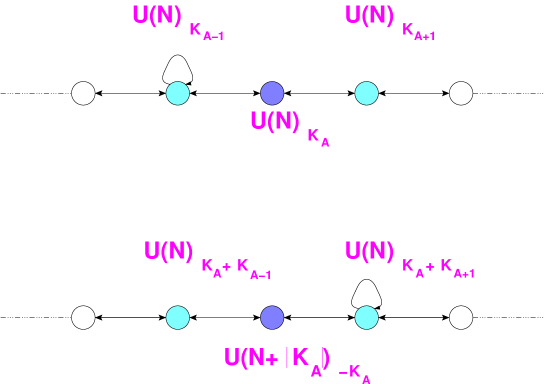
Figure 3: Dual phases describing a stack of M$2$ branes probing Calabi-Yau fourfold with adjoint matter involved in the duality.

The superpotential for the colored nodes of the quiver is

$$W_{e}=\dots+X_{A-1,A-1}X_{A-1,A}X_{A,A-1}-X_{A-1,A}X_{A,A+1}X_{A+1,A}X_{A,A-1}+\dots$$ (38)

The dual superpotential is

$$W_{m}=\dots Y_{A-1,A}Y_{A,A+1}Y_{A+1,A}Y_{A,A-1}-Y_{A+1,A+1}Y_{A+1,A}Y_{A,A+1}+\dots$$ (39)

The relevant contribution to the electric partition function on the squashed sphere is:

$$\mathcal{Z}_{e}= \frac{1}{\sqrt{\omega_{1}^{N}\omega_{2}^{N}}N!}\int\frac{\displaystyle\prod_{J=A-1}^{A}\prod_{i,j=1}^{N}\Gamma_{h}\left(\pm\left(x_{J}^{(i)}-x_{J+1}^{(j)}\right)+\omega\Delta_{J,J+1}^{(\eta)}\right)}{\displaystyle\prod_{J=A-1}^{A+1}\prod_{i<j}^{N}\Gamma_{h}\left(\pm\left(x_{J}^{(i)}-x_{J}^{(j)}\right)\right)}$$

$$\prod_{i,j=1}^{N}\Gamma_{h}\left(\pm\left(x_{i}^{(A-1)}-x_{i}^{(A-1)}\right)+\omega\Delta_{A-1,A-1}\right)\prod_{J=A-1}^{A+1}\prod_{i=1}^{N}c\left(-2k_{J}{x_{J}^{(i)}}^{2}\right)dx_{J}^{(i)}$$

The duality can be shown by following the same steps as in Subsection 4.1. The only difference is that in (34) there is an extra constraint $\Delta_{A-1,A-1}+\Delta_{A-1,A}+\Delta_{A,A-1}=2$. This constraint sets the contribution of the meson $Y_{A-1,A-1}$ to $1$ in the dual partition function (in field theory it is integrated out) because of (7).

4.2 The first class of orientilfolds: O$3$ planes

In this section we study the duality on the first class of orientifolded models introduced in section 3.2 and match the partition function between different phases. Recall that the relevant models are quiver field theories with alternating $"a"$ $SP(2N)_{k_{i}}$ and $"a"$ $SO(2N)_{2k_{i}}$ nodes, with $\sum k_{i}=0$. The superpotential is

$$W=\sum_{J=1}^{2a-1}\left(X_{J,J+1}\cdot X_{J+1,J+2}\right)^{2}$$ (41)

where $X_{2a,2a+1}=X_{2a,1}$. If $a>1$ there is always a field connecting two consecutive nodes labeled by $J$ and $J+1$, and we assign to this field the charge $\Delta_{J,J+1}$. The superpotential imposes the constraint $\Delta_{J-1,J}+\Delta_{J,J+1}=1$.

4.2.1 Duality on an $SP(2N)_{k}$ node

We first study the duality on an $SP(2N)_{k_{A}}$ group. Also in this case we refer to the quiver in Figure 2, but we erase the arrows because the groups are real and there is no distinction between fundamental and antifundamental representations. The relevant contribution to the partition function for this model is

$$\mathcal{Z}_{SP(2N)_{k_{A}}}=\int\frac{\displaystyle\prod_{J=A-1}^{A}\prod_{i,j=1}^{N}\Gamma_{h}\left(\pm x_{J}^{(i)}\pm x_{J+1}^{(j)}+\omega\Delta_{J,J+1}\right)\prod_{J=A-1}^{A+1}\prod_{i=1}^{N}c\left(-4k_{J}{x_{J}^{(i)}}^{2}\right)}{\displaystyle\prod_{1\leq i<j\leq N}\Gamma_{h}\left(\pm x_{A}^{(i)}\pm x_{A}^{(j)}\right)\prod_{i=1}^{N}\Gamma_{h}\left(\pm 2x_{A}^{(i)}\right)}\prod_{i=1}^{N}dx_{A}^{(i)}$$ (42)

where we used the notation $\Gamma_{h}(x+a)\Gamma_{h}(-x+a)=\Gamma_{h}(\pm x+a)$. In this case we define the $\mu_{r}$ variables as

$$\mu_{i,{A-1}}^{(\pm)}=\pm x_{A-1}^{(i)}+\omega\Delta_{A-1,A}\quad,\quad\mu_{i,{A+1}}^{(\pm)}=\pm x_{A+1}^{(i)}+\omega\Delta_{A,A+1}$$ (43)

Since there are $4N$ different $\mu$ the index $r$ runs from $1$ to $4N$, such that

$$\mu_{r}=\{\mu_{i,A-1}^{(+)},\mu_{i,A-1}^{(-)},\mu_{i,A+1}^{(+)},\mu_{i,A+1}^{(-)}\}$$ (44)

where every $i$ runs from $1$ to $N$. The dual gauge group is

$$SO(2N)_{2(k_{A-1}+k_{A})}\times SP(2(N+|k_{A}|-1))_{-k_{A}}\times SO(2N)_{2(k_{A}+k_{A+1})}$$ (45)

The dual superpotential is

$$W_{m}=Y_{A\pm 1,A\pm 1}\cdot Y_{A\pm 1,A}\cdot Y_{A,A\pm 1}-\left(Y_{A-1,A}\cdot Y_{A,A+1}\right)^{2}$$ (46)

The partition function of the dual gauge theory corresponds to the RHS of (A.2) by fixing $k_{A}>0$. In this case we have

$$I_{N,2(1+k_{A})a}^{N+k_{A}-1}(\mu)=I_{N+k_{A}-1,2(1+k_{A})b}^{N}(\omega-\mu)\prod_{1\leq r<s\leq 4N}\Gamma_{h}\left(\mu_{r}+\mu_{s}\right)\zeta^{(k_{A}-1)(1-2k_{A})}$$ (47)

$$c\left(\omega^{2}\left(2k_{A}^{2}\!-\!k_{A}\!\left(\!3\!+\!4N\!\left(\!\Delta_{A-1,A}^{2}\!+\!\Delta_{A,A+1}^{2}\!-\!1\!\right)\!\right)\!+\!1\right)\!-\!4k_{A}\left(\sum_{i=1}^{N}{x_{A-1}^{(i)}}^{2}\!+\!\sum_{i=1}^{N}{x_{A+1}^{(i)}}^{2}\!\right)\!\right)$$

The case $k_{A}<0$ in the electric theory is studied by inverting (A.2) as explained in Appendix A. As expected the rank of the dual groups is $\tilde{N}=N+|k_{A}|-1$.

It is straightforward to see from the first term in the RHS of (47) that the electric $R$-charge of a bifundamental connecting a pair of nodes in the electric theory is related in the magnetic theory to the $R$-charge of a bifundamental connecting the same pair of nodes nodes through $\widetilde{\Delta}_{i,j}=1-\Delta_{i,j}$.

The second term in the RHS of (47) can be expanded in terms of $\mu_{r}$ and it becomes

$$\prod_{1\leq r<s\leq 4N}\Gamma_{h}\left(\mu_{r}+\mu_{s}\right) =$$

$$= \prod_{1\leq i<j\leq N}\Gamma_{h}\left(\pm x^{(i)}_{A-1}\pm x^{(j)}_{A-1}+2\omega\Delta_{A-1,A}\right)\times{\Gamma_{h}}^{N}\left(2\omega\Delta_{A-1,A}\right)$$

$$\times \prod_{1\leq i<j\leq N}\Gamma_{h}\left(\pm x^{(i)}_{A+1}\pm x^{(j)}_{A+1}+2\omega\Delta_{A,A+1}\right)\times{\Gamma_{h}}^{N}\left(2\omega\Delta_{A,A+1}\right)$$

$$\times \,\,\,\,\,\prod_{i,j=1}^{N}\,\,\,\,\Gamma_{h}\left(\pm x^{(i)}_{A+1}\pm x^{(j)}_{A-1}+\omega\Delta_{A-1,A}+\omega\Delta_{A,A+1}\right)$$

The first two terms are the mesons of the dual theory while the last one evaluates to $1$ because of the superpotential constraint on the R-charges.

We conclude the proof of the duality with the analysis of the CS contributions to the partition function. The CS of the dual $SP$ group switches from $k_{A}$ to $-k_{A}$, because the dual theory is a “$b$” integral (see Appendix A for details). The CS of the $SO$ groups transform in (47) as $2k_{A\pm 1}\rightarrow 2k_{A}+2k_{A\pm 1}$, as expected.

Similar to the case of unitary theories, (47) also has which we ignore.

4.2.2 Duality on an $SO(2N)_{2k}$ node

In the O$3^{\pm}$ orientifolded quiver one can also dualize an $SO(2N)_{2k_{A}}$ node. The dual gauge group is

$$SP(2N)_{k_{A-1}+k_{A}}\times SO(2(N+|k|+1))_{-2k_{A}}\times SP(2N)_{k_{A}+k_{A+1}}$$ (50)

and the superpotential is again (46) with the proper products. The relevant contribution to the partition function of the electric theory is

$$\mathcal{Z}_{SO(2N)_{k_{A}}}=\int\frac{\displaystyle\prod_{J=A-1}^{A}\prod_{i,j=1}^{N}\Gamma_{h}\left(\pm x_{J}^{(i)}\pm x_{J+1}^{(j)}+\omega\Delta_{J,J+1}\right)\prod_{J=A-1}^{A+1}\prod_{i=1}^{N}c\left(-4k_{J}{x_{J}^{(i)}}^{2}\right)}{\displaystyle\prod_{1\leq i<j\leq N}\Gamma_{h}\left(\pm x_{A}^{(i)}\pm x_{A}^{(j)}\right)}\prod_{i=1}^{N}dx_{A}^{(i)}$$ (51)

As in Willett:2011gp ; Benini:2011mf the measure of the $SO(2N)$ gauge group can be converted into that of an $SP(2N)$ group by applying the relation (9) and inserting in the partition function the contribution

$$1=\frac{\displaystyle\prod_{i=1}^{N}\prod_{\alpha=1}^{4}\Gamma_{h}(\pm x_{A}^{(i)}+\rho_{\alpha})}{\Gamma_{h}({\pm 2x_{A}^{(i)}})}$$ (52)

where $\rho_{\alpha}=\left(0,\frac{\omega_{1}}{2},\frac{\omega_{2}}{2},\omega\right)$. The $\mu$ vector becomes

$$\mu_{r}=\{\mu_{i,A-1}^{(+)},\mu_{i,A-1}^{(-)},\mu_{i,A+1}^{(+)},\mu_{i,A+1}^{(-)},\rho_{\alpha}\}$$ (53)

where $r=1,\dots,4N+4$ and

$$\mu_{i,{A-1}}^{(\pm)}=\pm x_{A-1}^{(i)}+\omega\Delta_{A-1,A}\quad,\quad\mu_{i,{A+1}}^{(\pm)}=\pm x_{A+1}^{(i)}+\omega\Delta_{A,A+1}$$ (54)

By applying (A.2) with $k_{A}>0$ we have

$$I_{N,2(1+k_{A})_{a}}^{N+k_{A}+1}(\mu) = I_{N+k_{A}+1,2(1+k_{A})_{b}}^{N}(\omega-\mu)\prod_{1\leq r<s\leq 4N+4}\Gamma_{h}\left(\mu_{r}+\mu_{s}\right)\zeta^{(k_{A}-1)(1-2k_{A})}$$

$$\times c\left(4k_{A}\left(\sum_{i=1}^{N}{x_{A-1}^{(i)}}^{2}+\sum_{i=1}^{N}{x_{A+1}^{(i)}}^{2}\right)-\frac{1}{2}k_{A}\left(\omega_{1}{}^{2}+\omega_{1}{}^{2}\right)\right)$$

$$\times c\left(\omega^{2}\left(2k_{A}{}^{2}+k_{A}\left(3-4N\left(\Delta_{A-1,A}{}^{2}+\Delta_{A,A+1}{}^{2}-1\right)\right)+1\right)\right)$$

The case $k_{A}<0$ in the electric theory is studied by inverting (A.2). As expected the rank of the dual groups is $\tilde{N}=N+|k_{A}|+1$. Observe that it fits with the proposal of Kapustin:2011vz , $SO(\tilde{N}_{c})=SO(N_{f}+|K|-2-N_{c})$. Indeed in our case $N_{c}=2N$, $K=2k_{A}$, $N_{f}=4N+4$ and $\tilde{N}_{c}=2(N+|k_{A}|+1)$.

The RHS of (4.2.2) corresponds to the partition function of the dual theory. By using the relation (52) the extra terms in the measure arising in (4.2.2) become

$$\frac{\displaystyle\prod_{i=1}^{N+|k_{a}|+1}\prod_{\alpha=1}^{4}\Gamma_{h}(\omega\pm x_{A}^{(i)}-\rho_{\alpha})}{\Gamma_{h}({\pm 2x_{A}^{(i)}})}=1$$ (56)

thus giving us the measure of the $SO(2(N+|k_{A}|+1))$ dual gauge group.

Upon expanding the $\Gamma_{h}(\mu_{r}+\mu_{s})$ term in the RHS of (4.2.2) we find

$$\prod_{1\leq r<s\leq 4N+4}\Gamma_{h}\left(\mu_{r}+\mu_{s}\right)=\prod_{1\leq r<s\leq 4N}\Gamma_{h}\left(\mu_{r}+\mu_{s}\right)\prod_{{\tiny\begin{array}[]{c}1\leq r\leq 4N\\ 4N<s<4N+4\end{array}}}\Gamma_{h}\left(\mu_{r}+\mu_{s}\right)\prod_{4N<r<s\leq 4N+4}\Gamma_{h}\left(\mu_{r}+\mu_{s}\right)$$ (59)

By combining the first two products we obtain

$$\prod_{i,j=1}^{N}\Gamma_{h}(\pm x_{A+1}^{(i)}\pm x_{A+1}^{(j)}+2\omega\Delta_{A,A+1})\times\prod_{i,j=1}^{N}\Gamma_{h}(\pm x_{A-1}^{(i)}\pm x_{A-1}^{(j)}+2\omega\Delta_{A-1,A})$$ (61)

which represent the massless mesons of dual theory (they are the adjoints of neighbouring SP$(2N)$). The extra contributions from the first two terms in the RHS of (59) correspond to the massive mesons and evaluate to $1$. The last term in the product in (59) is

$$\Gamma_{h}\left(\frac{\omega_{1}}{2}\right)\Gamma_{h}\left(\frac{\omega_{2}}{2}\right)\Gamma_{h}(\omega)^{2}\Gamma_{h}\left(\omega+\frac{\omega_{1}}{2}\right)\Gamma_{h}\left(\omega+\frac{\omega_{2}}{2}\right)=1$$ (62)

bacause of (8). The rest of the terms in (4.2.2) give the right transformation on the $CS$ levels and an extra phase as usual.

4.3 The second class of orientifolds: duality on $SO(2N+1)_{k}$

If we consider $\widetilde{\text{O}3}^{\pm}$ orientifold planes, the gauge groups of the necklace quiver involve $SO(2N+1)$ factors instead of $SO(2N)$. We are interested in studying the duality on these nodes. The relevant contribution to the partition function is

$$\mathcal{Z}_{SO(2N+1)_{k_{A}}} = \int\frac{\displaystyle\prod_{J=A-1}^{A}\prod_{i,j=1}^{N}\Gamma_{h}\left(\pm x_{J}^{(i)}\pm x_{J+1}^{(j)}+\omega\Delta_{J,J+1}\right)\prod_{J=A-1}^{A+1}\prod_{i=1}^{N}c\left(-4k_{J}{x_{J}^{(i)}}^{2}\right)}{\displaystyle\prod_{1\leq i<j\leq N}\Gamma_{h}\left(\pm x_{A}^{(i)}\pm x_{A}^{(j)}\right)\prod_{i=1}^{N}\Gamma_{h}\left(\pm x_{A}^{(i)}\right)}$$ (63)

$$\times \prod_{i=1}^{N}\Gamma_{h}\left(\pm x_{A-1}^{(i)}+\omega\Delta_{A-1,A}\right)\Gamma_{h}\left(\pm x_{A+1}^{(i)}+\omega\Delta_{A,A+1}\right)dx_{A}^{(i)}$$

The measure of the $SO(2N+1)$ group can be converted into the one of an $SP(2N)$ group by applying (9). We find

$$\frac{1}{\Gamma_{h}\left({\pm x_{A}^{(i)}}\right)}=\frac{\Gamma_{h}\left(\pm x_{A}^{(i)}+\frac{\omega_{1}}{2}\right)\Gamma_{h}\left(\pm x_{A}^{(i)}+\frac{\omega_{2}}{2}\right)}{\Gamma_{h}\left(\pm 2x_{A}^{(i)}\right)}$$ (64)

In this case the $\mu$ vector is $4N+2$ dimensionful. The first $4N$ elements are the same of the previous orthogonal case while the extra two are $\frac{\omega_{1}}{2}$ and $\frac{\omega_{2}}{2}$.

The partition function of the dual theory is obtained by applying (A.2) to (63). By fixing $k_{A}>0$ we have

$$I_{N,2(1+k_{A})_{a}}^{N+k_{A}}(\mu) = I_{N+k_{A},2(1+k_{A})_{b}}^{N}(\omega-\mu)\prod_{1\leq r<s\leq 4N+2}\Gamma_{h}\left(\mu_{r}+\mu_{s}\right)\zeta^{(k_{A}+1)(1-2k_{A})}$$

$$\times c\left(-4k_{A}\left(\sum_{i=1}^{N}{x_{A-1}^{(i)}}^{2}+\sum_{i=1}^{N}{x_{A+1}^{(i)}}^{2}\right)-\frac{1}{2}k_{A}\left(\omega_{1}^{2}+\omega_{2}^{2}\right)\right)$$

$$\times c\left(\omega^{2}k_{A}\left(2k_{A}+1+4N-4N\left(\Delta_{A-1,A}^{2}+\Delta_{A,A+1}^{2}\right)\right)\right)$$

The case $k_{A}<0$ in the electric theory is studied by inverting (A.2). As expected the rank of the dual group is $\tilde{N}=N+|k_{A}|$. Observe that it fits with the proposal of Kapustin:2011vz , $SO(\tilde{N}_{c})=SO(N_{f}+|K|-2-N_{c})$. Indeed in our case $N_{c}=2N+1$, $K=2k_{A}$, $N_{f}=4N+2$ and $\tilde{N}_{c}=2(N+|k_{A}|)+1$.

As before we can transform the measure back to $SO(2(N+|k_{A}|)+1)$ by applying (64). Then we study the mesons: we have to expand the product

$$\prod_{1\leq r<s\leq 4N+2}\Gamma_{h}\left(\mu_{r}+\mu_{s}\right)\times\prod_{1\leq r\leq 4N}\Gamma_{h}\left(\mu_{r}\right)$$ (66)

where the first term come from (4.3) and the second one from (63). It is not difficult to recognize the contribution of the dual mesons predicted by the duality. The term $1\leq r<s\leq 4N$ gives

$$\prod_{1\leq i<j\leq N}\Gamma_{h}(\pm x_{A\pm 1}^{(i)}\pm x_{A\pm 1}^{(j)}+2\omega\Delta_{A,A\pm 1})$$ (67)

The extra contributions come from

$$\prod_{1\leq r<\leq 4N,4N<s\leq 4N+2}\Gamma_{h}\left(\mu_{r}+\mu_{s}\right)\times\prod_{1\leq r\leq 4N}\Gamma_{h}\left(\mu_{r}\right)$$ (68)

Explicitly we have

$$\prod_{i=1}^{N}\left(\prod_{\alpha=1,2}\Gamma_{h}\left(\pm x_{A\pm 1}^{(i)}+\omega\Delta_{A\pm 1}+\frac{\omega_{\alpha}}{2}\right)\right)\times\Gamma_{h}\left(\pm x_{A\pm 1}^{(i)}+\omega\Delta_{A\pm 1}\right)=$$

$$= \frac{\Gamma_{h}\left(\pm 2x_{A\pm 1}+\omega\Delta_{A\pm 1,A}\right)}{\Gamma_{h}\left(\pm x_{A\pm 1}+\omega\Delta_{A\pm 1,A}+\omega\right)}$$ (69)

The numerator in this expression replaces $i<j$ with $i\leq j$ in (67) while the denominator can be transformed as

$$\frac{1}{\Gamma_{h}\left(\pm x_{A\pm 1}+\omega\Delta_{A\pm 1,A}+\omega\right)}=\Gamma_{h}\left(\pm x_{A\pm 1}+\omega(1-\Delta_{A\pm 1,A})\right)$$ (70)

which corresponds to the dual of the second line of (63).

5 Duality and free theories: some exact results

Three dimensional dualities are not only important for theories with an AdS dual but also for more general SCFTs. For example in Jafferis:2011ns a new duality was proposed between an $SU(2)_{1}$ CS theory with an adjoint and no superpotential and a free theory. This duality was further studied in Kapustin:2011vz , in which an interacting CS matter theory without superpotential is dual to a free theory. While many checks have been performed by expanding the superconformal index, and comparing the expansions on both sides of the dualities, a full understanding of the matching of the partition function is still missing. Here we show the matching between the partition functions analytically.

The models considered in this section do not suffer from accidental symmetries. In every case the partition function matrix integral of the electric interacting theory can be worked out exactly and the extremization of the result sets the $R$-charges of the magnetic fields to the canonical value without any modification. In general, the naive extremization does not give this result, because the $R$-symmetry mixes with accidental symmetries. We comment on the latter cases in the next section.

A technical comment is in order. In the following we need some relations involving the integrals dubbed as JI in appendix A. We take them from fvdb and mention them in the text when necessary.

5.1 $SU(2)_{1}$ theory with an adjoint field

The first example is an $SU(2)_{1}$ CS theory with an adjoint, studied in Jafferis:2011ns . The authors proposed a general formula for the partition function in this case but they did not prove this formula analytically. Here we use the results of fvdb to show the agreement. The partition function on the round sphere is

$$Z_{SU(2)_{1}}(\Delta) = \int dx\sinh^{2}\left(2\pi x\right)e^{2\pi ix^{2}}e^{l(1-\Delta)+l(1-\Delta+2ix)+l(1-\Delta-2ix)}$$

$$= \frac{1}{4}\int d\epsilon\int dx_{1}dx_{2}\left(-4\sin(\frac{\pi(x_{1}-x_{2})}{i})\sin(\frac{\pi(x_{1}-x_{2})}{i})\right)$$

$$e^{\pi i(x_{1}^{2}+x_{2}^{2})}e^{l(1+i\tau)+l(1+i\tau+i(x_{1}-x_{2}))+l(1+i\tau-i(x_{1}-x_{2}))}e^{2\pi i(x_{1}+x_{2})\epsilon}$$

where we used the relation

$$\int d\,x_{1}d\,x_{2}\delta(x_{1}+x_{2})=\int d\epsilon\int d\,x_{1}d\,x_{2}e^{2\pi i(x_{1}+x_{2})\epsilon}$$ (72)

and we set $\tau=i\Delta$, where $\Delta$ represents the $R$-charge of the adjoint field. In terms of the hyperbolic functions the partition function becomes

$$Z_{SU(2)_{1}}(\Delta)= -\frac{1}{4\Gamma_{h}^{\prime}(\tau)}\int d\epsilon\Bigg{(}\frac{\Gamma_{h}^{\prime}(\tau)^{2}}{2}\int d\,x_{1}d\,x_{2}\frac{\Gamma_{h}^{\prime}(\tau\pm(x_{1}-x_{2}))}{\Gamma_{h}^{\prime}(\pm(x_{1}-x_{2})}$$ (73)

$$\times c^{\prime}(2\lambda(x_{1}+x_{2})-2(x_{1}^{2}+x_{2}^{2}))\Bigg{)}$$

where $\lambda=-2\epsilon$. We used the notations $\Gamma_{h}^{\prime}$ and $c^{\prime}$ to specify that we are considering $\omega_{1}=\omega_{2}=i$, i.e. this is the partition function on the three sphere. More generally the formula inside the parenthesis can be associated to the partition function on the squashed three sphere, and the resulting integral has been computed in fvdb . Here we quote the result

$$\frac{\Gamma_{h}(\tau)^{n}}{\sqrt{\left(-\omega_{1}\omega_{2}\right)^{n}}n!}\int\prod_{1<\leq i\leq j\leq n}\frac{\Gamma_{h}(\tau\pm(x_{i}-x_{j})}{\Gamma_{h}(\pm(x_{i}-x_{j}))}\prod_{j=1}^{n}c(2\lambda x_{j}-2x_{j}^{2})dx_{j}=$$

$$= \zeta^{-3n}\prod_{j=1}^{n}\Gamma_{h}\left(j\tau\right)c\left(\frac{n}{2}\left(2\omega^{2}+\lambda^{2}+2(n-1)\tau\omega+\frac{1}{3}(n-1)(2n-1)\tau^{2}\right)\right)$$ (74)

By reducing on the three sphere, fixing $n=2$ and applying (5.1) we have

$$Z_{SU(2)_{1}}=-\frac{1}{4\Gamma_{h}^{\prime}(\tau)}\int d\epsilon\,\,\,{\zeta^{\prime}}^{-6}\Gamma_{h}^{\prime}(\tau)\Gamma_{h}^{\prime}(2\tau)c^{\prime}\left(-2+\lambda^{2}+2i\tau+\tau^{2}\right)$$ (75)

If we substitue $\zeta^{\prime}=e^{i\pi/12}$ and $\tau=i\Delta$ in (75) and perform the gaussian integration

$$\int_{-\infty}^{\infty}d\,\lambda e^{-\frac{i\pi\lambda^{2}}{2}}=\frac{2}{\sqrt{2}}e^{-\frac{i\pi}{4}}$$ (76)

the final expression becomes

$$Z_{SU(2)_{1}}=\frac{1}{2\sqrt{2}}e^{l(1-2\Delta)}e^{\frac{i\pi}{2}(1+\Delta)^{2}-\frac{i\pi}{4}}$$ (77)

which coincides with the one proposed by Jafferis:2011ns .

5.2 SO$(4)_{1}$ with the adjoint field

As discussed in Kapustin:2011vz , the $SO(4)_{1}$ with an adjoint reduces to two copies of the Jafferis:2011ns duality, because $SO(4)\simeq SU(2)\times SU(2)$. Here we show that the partition function can be exactly computed in the $SO$ cases by using the results of fvdb and reproduce the $SO(4)_{1}$ case explicitly. In this case we need the relation

$$\frac{\Gamma_{h}(\tau)^{n}}{\sqrt{\left(\omega_{1}\omega_{2}\right)^{n}}2^{n}n}\int\frac{\displaystyle\prod_{1\leq i<j\leq n}\Gamma_{h}(\tau\pm x_{i}\pm x_{j})\prod_{j=1}^{n}\prod_{r=1}^{3}\Gamma_{h}(\mu_{r}\pm x_{j})}{\displaystyle\prod_{1\leq i<j\leq n}\Gamma_{h}(\pm x_{i}\pm x_{j})\prod_{j=1}^{n}\Gamma_{h}(\pm 2x_{j})}\prod_{j=1}^{n}c(-2x_{j}^{2})dx_{j}=$$

$$= \prod_{j=1}^{n}\Gamma_{h}(j\tau)\prod_{1\leq r<s\leq 3}\Gamma_{h}(j\tau+\mu_{r}+\mu_{s})$$ (78)

$$\times c\left(n\left(2(\mu_{0}\mu_{1}+\mu_{1}\mu_{2}+\mu_{2}\mu_{0})+2(n-1)\tau\sum_{r=1}^{3}\mu_{r}+\frac{1}{3}(n-1)(4n-5)\tau^{2}\right)\right)$$

This equation can be applied to the SO$(2n)_{1}$ case after we identify

$$\mu_{1}=0\quad,\quad\mu_{2}=\frac{\omega_{1}}{2}\quad,\quad\mu_{3}=\frac{\omega_{2}}{2}$$ (79)

because, by applying (7) and (9), we have

$$\frac{\Gamma_{h}\left(\pm x\right)\Gamma_{h}\left(\pm x+\frac{\omega_{1}}{2}\right)\Gamma_{h}\left(\pm x+\frac{\omega_{2}}{2}\right)}{\Gamma_{h}(\pm 2x)}=1$$ (80)

Formula (5.2) then reduces to the partition function of a SO$(2n)_{1}$ theory with a field in the adjoint representation. If we reduce to the case $n=2$ and fix $\tau=i\Delta$ and $\omega_{1}=\omega_{2}=i$ the partition function on the three sphere is

$$e^{2l(1-2\Delta)}e^{2\pi i\left(\Delta+\frac{1}{2}\right)^{2}-\frac{3}{2}\pi i}$$ (81)

which reduces to two copies of $SU(2)_{1}$ theories with the adjoint and differs from that case just by a phase factor.

5.3 $SP(4)_{2}$ with an absolutely antisymmetric field

In the case of symplectic groups also there are exact relations in fvdb that can be applied to obtain a CS matter theory dual to a free theory.

Here we study the irreducible absolutely antisymmetric representation, described by the Dynkin label $\vec{s}=(1,1,0\dots,0)$ (see Appendix B for details). By using the Schur polynomial in the appendix the character of this irreducible representation is

$$\chi_{(1,1,0,\dots,0)}=\sum_{i\neq j}\left(z^{i}z^{j}+z^{i}z^{-j}+z^{-i}z^{j}+z^{-i}z^{-j}\right)+N-1$$ (82)

In this case we need the equality fvdb

$$\frac{\displaystyle\Gamma_{h}(\tau)^{n-1}}{\sqrt{\left(-\omega_{1}\omega_{2}\right)^{n}}2^{n}n!}\int\prod_{1\leq i<j\leq n}\frac{\Gamma_{h}(\tau\pm x_{i}\pm x_{j})}{\Gamma_{h}(\pm x_{i}\pm x_{j})}\prod_{j=1}^{n}\frac{1}{\Gamma_{h}(\pm 2x_{j})}c(-8x_{j}^{2})dx_{j}=$$

$$= \zeta^{-3n}\prod_{j=2}^{n}\Gamma_{h}(j\tau)\,c\left(n\left(3\omega^{2}+3(n-1)\tau\omega+\frac{1}{6}(n-1)(2n-7)\tau^{2}\right)\right)$$ (83)

For $n=2$ it represents the partition function for a $SP(4)_{2}$ gauge theory with an absolutely antisymmetric two index tensor. By fixing $\tau=i\Delta$ and $\omega_{1}=\omega_{2}=i$ the partition function on the three sphere becomes

$$\mathcal{Z}_{SP(4)_{2}}=e^{l(1-2\Delta)}e^{-\frac{i\pi}{2}(\Delta-3)^{2}}$$ (84)

This relation suggests that this theory is dual to a free theory with a singlet.

A similar duality appeared in Kapustin:2011vz , however the antisymmetric representation considered there was not irreducible and contained another singlet. This extra singlet adds a $\Gamma_{h}(\tau)$ factor on both sides of (84), leaving the equality unchanged. In this case the theory is dual to a theory with two singlets with charges $\Delta$ and $2\Delta$. This case contains accidental symmetries which mix wit the $R$-symmetry and need to be properly accounted in the extremization of the partition function. We will comment on this issue in section 6.

5.3.1 The superconformal index

The superconformal index is a Witten like index which counts over the protected BPS states of the theory. The index for three dimensional theories with $\mathcal{N}\geq 3$ SUSY was first proposed in Bhattacharya:2008bja by localizing the theory on on $S^{2}\times S^{1}$. The expression for the index is given by

$$\mathcal{I}(x,y_{i})=\text{Tr}(-1)^{F}x^{E+j_{3}}\prod_{i}y_{i}^{F_{i}}$$ (85)

where $F$ is the fermion number, E is the energy, $j_{3}$ is the third component of the $SU(2)$ rotational symmetry in the superconformal group. This index was refined to include the monopole contributions in Kim:2009wb . For theories with $\mathcal{N}=2$ supersymmetry the $R$-charge is not constrained to be canonical anymore, and the index for a generic $R$-charge assignment was found in Imamura:2011su . It is important to observe that, in the general case, dual theories share the same index only after the contribution from the monopole sectors is included. In some cases the index matches sector by sector but in general one has to sum over all the sectors. For example if an interacting theory is dual to a free theory one has to necessarily include the monopole corrections before matching the indices.

Here we consider the index of the $SP(4)_{2}$ CS theory with one matter field in the absolutely antisymmetric representation and $R$-charge $\Delta$. After including the contribution from monopoles with GNO charge $(1,0)$ the superconformal index is

$$\mathcal{I} = \left(1-x^{2}+x^{2\Delta}+x^{4\Delta}+x^{6\Delta}+x^{8\Delta}+x^{10\Delta}+x^{12\Delta}+x^{14\Delta}+\dots\right){}_{(0,0)}$$

$$+ \left(-x^{2-2\Delta}-x^{4-2\Delta}+\dots\right){}_{(1,0)}+\dots$$

$$= 1-x^{2}-x^{2-2\Delta}-x^{4-2\Delta}+x^{2\Delta}+x^{4\Delta}+x^{6\Delta}+x^{8\Delta}+x^{10\Delta}+x^{12\Delta}+x^{14\Delta}+\dots$$

This coincides with the index of a free multiplet with $R$-charge $2\Delta$, corroborating the duality proposed above.

6 Comments on accidental symmetries

In this section we briefly comment on a proposal to deal with accidental symmetries in three-dimensional field theories. We will adapt to the three-dimensional case a similar prescription used in the four-dimensional $a$-maximization Kutasov:2003iy , with the respective physical meaning Barnes:2004jj , which also allows for an extension away from the fixed points Amariti:2011xp based on the four dimensional analogy Kutasov:2003ux . For a preliminary discussion, see Morita:2011cs .

Any time the fixed point scaling dimension of a scalar gauge invariant operator drops below the $d$-dimensional unitary bound $\Delta\geq(d-2)/2$, this signals that the UV description that we are using to extract information about the IR physics is no longer valid, because the theory enjoys new ”accidental” symmetries which are not manifest in the UV description. The new symmetries are generated by the gauge invariant operators, which decouple from the rest of the theory in the IR: they retain their canonical scaling dimensions and describe free fields. In these cases we need to modify the UV description in a suitable way, which we describe in the following.

Consider a model where $m$ gauge invariant operators ${\cal O}_{i}$, $i=1,\ldots,m$ hit the unitary bound, and consider coupling to that theory $m$ sources $L_{i}$ and $m$ gauge invariant operators $M_{i}$ through the superpotential

$$\Delta W=L^{i}\left({\cal O}_{i}+\lambda M_{i}\right)$$ (87)

where $\lambda$ is small in the UV. The operators ${\cal O}_{i}$ are, in general, not related to each other, and so are the $L$’s and the $M$’s. Imposing the condition $R(L_{i})+R({\cal O}_{i})=2$ we see that when $R({\cal O}_{i})>(d-2)/(d-1)$ the last term is indeed relevant and makes the fields $L$ and $M$ massive. Once they are integrated out, we obtain the IR superconformal theory we started with, and no physical quantity has changed. On the other hand, when $R({\cal O}_{i})<(d-2)/(d-1)$, the $LM$ coupling is irrelevant and the $M$’s are free decoupled fields in the IR.

In the case of three-dimensional field theories, where $R=\Delta$, a free field contributes a factor $\exp\left(\ell(1/2)\right)=2^{-1/2}$ to the partition function, or equivalently a term $\log(2)/2$ to the free energy. The $R$-charge of the $L$’s is fixed by the first term in (87), and their contribution to the partition function is $\exp\left(m\ell(-1+\Delta({\cal O})\right)$. Summing everything up, we obtain

$$F=F_{0}+\left(m\frac{\log(2)}{2}+\sum_{i=1}^{m}\ell\left(1-\Delta({\cal O}_{i})\right)\right)$$ (88)

where we also used $\ell(1-\Delta)=-\ell(-1+\Delta)$ for $0<\Delta<2$, which is always the case in any sensible theory (see footnote 9). Equation (88) has a very clear interpretation: along the RG flow, the $R$-charges as a function of the RG scale are given by the Lagrange multiplier technique Amariti:2011xp ; when a gauge invariant operator hits the unitary bound, one subtracts its contribution to the free energy and adds the contribution of the same number of free fields. Because both the correction term to (88) and its first derivative vanish at the free field point $\Delta({\cal O}_{i})=1/2$, all the $R$-charges and the free energy itself are continuous and differentiable functions of the RG scale.

6.1 Accidental symmetries in the duality with free theories

In section 5 we focused on theories with a free magnetic dual whose partition function can be exactly and consistently computed by localization and extremization without any further modification. We now apply the discussion in the previous subsection and show how the computation of the exact superconformal $R$-charge can be consistently worked out even when the infrared theory enjoys accidental symmetries. This provides new and stronger checks of three-dimensional dualities.

We start by describing an example in some detail, in which the dual gauge group vanishes and the magnetic theory only contains a tower of non-interacting singlets with naive $R$-charges different from the canonical ones. The simplest electric theory of this kind has $U(N_{c})_{1}$ gauge group and contains one adjoint $X$ with a vanishing superpotential Kapustin:2011vz .

The partition function of the $U(N_{c})_{1}$ theory with one adjoint $X$ can be exactly computed fvdb

$$\mathcal{Z}_{U(N_{c})_{1},X}=e^{\frac{i\pi}{12}N\left(3+6\Delta\left(N_{c}-1\right)+\Delta^{2}\left(2N_{c}^{2}-3N_{c}+1\right)\right)}\times\prod_{j=1}^{N_{c}}e^{l(1-j\Delta)}$$ (89)

where $j\Delta$ is the $R$-charge of Tr$X^{j}$. Notice that the $U(1)\subset U(N_{c})$ decouples and Tr$X$ is a free field. However, for the sake of uniform treatment, we keep its $R$-charge to be $\Delta$ instead of $1/2$.

The naive $R$ charges of the $N_{c}$ free fields of the magnetic theory, given by $u_{j}=$Tr$X^{j}$, are obtained by extremizing (89), which boils down to solving the equation

$$\frac{\partial\log\left|\mathcal{Z}_{U(N_{c})_{1},X}(\Delta,N_{c})\right|}{\partial\Delta}=\sum_{j=1}^{N_{c}}j\pi(1-j\Delta)\cot(\pi(1-j\Delta))=0$$ (90)

The solution is

$$\Delta=\frac{1}{N_{c}+1}$$ (91)

Proving that (91) solves (90) is pretty straightforward. Indeed

$$\left.\frac{\partial\log\left|\mathcal{Z}_{U(N_{c})_{1},X}(\Delta,N_{c})\right|}{\partial\Delta}\right|_{\Delta=\frac{1}{N_{c}+1}}=\sum_{j=1}^{N_{c}}\left(\frac{j(N_{c}+1-j)}{N_{c}+1}\right)\cot\left(\frac{j\,\pi}{N_{c}+1}\right)=$$

$$= \frac{1}{2}\left(\sum_{j=1}^{N_{c}}\left(\frac{j(N_{c}+1-j)}{N_{c}+1}\right)\cot\left(\frac{j\,\pi}{N_{c}+1}\right)+\left(j\rightarrow N_{c}+1-j^{\prime}\right)\right)=0$$ (92)

It follows that the singlets do not have the canonical scaling dimension, and there are $\left[\frac{N_{c}+1}{2}\right]$ gauge invariant operators with $R$-charge below or at the unitarity bound; thus, we have to treat them as free fields, and modify the extremization principle according to equation (88). We interpret this first step by noticing that along the RG flow, the operators ${\rm Tr}X^{j}$ with $j<\left[\frac{N_{c}+1}{2}\right]$ will hit the unitarity bound at higher energies. For high enough $N_{c}$, this is not the end of the story: extremization of the modified free energy shows that we did not cure all the accidental symmetries. Again, roughly half of the operators have $R$-charges below or at the unitarity bound, and we again apply (88). The process continues until all but one operator, namely $u_{N_{c}}$, remains and we end up with the following modified partition function

$$\left|\mathcal{Z}_{U(N_{c})_{1},X}\right|=2^{-\frac{N_{c}-1}{2}}e^{l(1-N_{c}\Delta)}$$ (93)

which is extremized at $N_{c}\Delta=1/2$. We have then shown that the $U(N_{c})_{1}$ partition function coincides with the one of $N_{c}$ free fields $u_{j}$, and that a proper treatment of the accidental symmetries allows us to identify the duality map as $u_{j}={\rm Tr}X^{j}$. The same arguments may be carried over to other models.

7 Open questions

We provided some nontrivial evidence for classes of infinite three-dimensional dualities for theories with unitary, orthogonal and symplectic gauge groups. Our results provide support for arbitrary gauge group and CS levels, and extend previous results which were limited either to the large-$N$ limit or to numerical evaluations for low ranks and one factor in the gauge group.

Our main tool has been the exact, all-loop partition function evaluated on a squashed three sphere. Allowing for arbitrary $R$-charges, it can be written as an integral of hyperbolic functions which have been recently studied by mathematicians.

Exact evaluation of the above quantities, available in the literature for classical gauge groups, allowed to uncover new dualities. In the large-$N$ limit, and for low enough CS levels, they could also be inferred by the AdS/CFT duality, and exact evaluation of the above quantities allows for an extension to arbitrary ranks and levels.

Unitary gauge groups have been extensively studied in the large-$N$ limit, and precise prescriptions for the computation of the partition function in this regime are available in the literature. Because of its simplifying nature, it is much more tractable than the computation of the finite-$N$ partition function and it allows for comparison of physical quantities in the AdS/CFT correspondence. Based on this observation, we tried analyzing the case of the other classical gauge groups, where a similar analysis still lacks. We found that the set of saddle point equations are not consistent with the long range cancellation in these cases. Thus, the continuum limit would require a different approach. A similar situation also holds in chiral-like models for unitary gauge groups Amariti:2011jp ; Amariti:2011uw . There exist other dualities between quivers with unitary gauge groups and quivers with symplectic/orthogonal gauge groups Aharony:2008gk . These dualities suggest that the theories with symplectic and orthogonal groups also exhibit the $N^{3/2}$ scaling of the free energy at large $N$. It will be interesting to prove the matching of the partition function for these dualities along the lines of this paper.

Some of the dualities we have studied involve free field theories on the magnetic side. Some comments are in order. Any nontrivial check involving the partition function in this case requires the possibility of an exact evaluation of the full matrix integral, because on the free theory side there is no integral at all. Secondly, when one considers such theories, it turns out that the free theory contains $n$ free fields with charge $j\Delta$, with $\Delta$ the smallest charge and $j=1,\ldots,n$. While this constitutes an offshell check of the duality, we know that a free field has $R$-charge $1/2$, which cannot be obtained by extremization of the naive partition function. If the duality holds, this means that the electric $R$-symmetry mixes with an accidental symmetry and we showed how to handle this scenario in Section 6.

More generally accidental symmetries arise in presence of gauge theories with tensor matter and superpotential Kapustin:2011vz . These dualities are three dimensional generalizations of the KSS dualities Kutasov:1995ss . It would be interesting to study the matching of the partition functions in these cases, as already proposed in Morita:2011cs , at finite values for the ranks of the gauge groups and CS level.

We conclude by recalling that accidental symmetries are one of the main issue in the proof of a $c$-theorem. In the three dimensional case the candidate $c$-function in is the free energy $F$ on the round $S^{3}$ ($F=-\log|\mathcal{Z}|$), which has been conjecture to decrease along the RG flow Jafferis:2011zi . Relevant deformations break the abelian symmetries which are manifest in the UV description of the theory and once we have a quantity that is maximized by the exact superconformal $R$-symmetry we can interpret it as the $c$-function. The $c$-theorem immediately follows from the two line ”almost proof” of Intriligator:2003jj . However accidental symmetries constitute a loophole to this argument and a proof of the $F$-theorem requires more care in this case: the free field value is a maximum for the function $-\ell(1-\Delta)$, thus the infrared correction term in (88) is always positive, for any value of the scaling dimensions, in full agreement with the maximization of $F$. However, the correction term adds a positive contribution to $F_{IR}$, possibly invalidating the $F$-theorem $F_{IR}<F_{UV}$.

Appendix A Relations among hyperbolic integrals

In this appendix we review the equivalence among the hyperbolic integrals necessary to match the dual phases in the quiver gauge theories that we studied in the paper. We refer to fvdb for more details.

A.1 The unitary case

The partition function for a $U(n)$ gauge theory with CS level $2t$, $s_{1}$ fundamentals, $s_{2}$ anti-fundamentals and one adjoint matter field corresponds to the integral dubbed as $\textit{JI}_{n,(s_{1},s_{2}),t}(\mu;\nu;\lambda;\tau)$ in fvdb . The original integral is defined as

$$\textit{JI}_{n,(s_{1},s_{2}),t}(\mu;\nu;\lambda;\tau) =\frac{\Gamma_{h}(\tau)^{n}}{\sqrt{-\omega_{1}\omega_{2}}^{n}n!}\int\prod_{i\leq j<k\leq n}\frac{\Gamma_{h}(\tau\pm(x_{j}-x_{k}))}{\Gamma_{h}(\pm(x_{j}-x_{k}))}$$

$$\times\prod_{j=1}^{n}\prod_{r=1}^{s_{1}}\Gamma_{h}(\mu_{r}-x_{j})\prod_{s=1}^{s_{2}}\Gamma_{h}(\nu_{s}+x_{j})c(2\lambda x_{j}+tx_{j}^{2})dx_{j}$$

The variables $\tau$, $\nu$ and $\mu$ are linear combinations of the chemical potentials for the global symmetries under which the adjoint, fundamental and anti-fundamental fields are charged respectively.

In the cases studied in section 4 the theory does not contain an adjoint. This corresponds to identifying the parameter $\tau$ with $\omega$. In the hyperbolic function analysis, setting $\tau=\omega$, removes the adjoint field contributions from the above integral because of (7) and (8). The new integral is defined as

$$\textit{J}_{n,(s_{1},s_{2}),t}(\mu;\nu;\lambda)=\textit{JI}_{n,(s_{1},s_{2}),t}(\mu;\nu;\lambda;\omega)$$ (94)

The field theory duality is translated in an equivalence between the integrals in (94). These equivalences are derived from the transformation properties of certain integrals named degenerations in fvdb

$$\textit{I}_{n,\xi}^{m}(\mu;\nu;\lambda)=\textit{J}_{n,(s_{1},s_{2}),t}(\mu;\nu;\lambda)$$ (95)

where $\xi$ labels the integrals on the LHS of (95). The value taken by $\xi$ is either (p,q)$a$ or (p,q)$b$ and it can be fixed by using the following table

condition	type	$m$	p	q
$t<-|s_{1}-s_{2}|$	$\text{(p,q)}a$	$\frac{s_{1}+s_{2}-t-2n}{2}$	$\frac{s_{1}-s_{2}-t+4}{2}$	$\frac{s_{2}-s_{1}-t+4}{2}$
$t>|s_{1}-s_{2}|$	$\text{(p,q)}b$	$\frac{s_{1}+s_{2}+t-2n}{2}$	$\frac{s_{2}-s_{1}+t+4}{2}$	$\frac{s_{1}-s_{2}+t+4}{2}$

Even if the definition of $\textit{I}_{n,\xi}^{m}$ looks like a re-parametrization of $\textit{J}_{n,(s_{1},s_{2}),t}\,$, the equality (95) is valid only under certain very broad conditions on the $\mu$, $\nu$ and $\tau$ variables . At this point of the discussion we prefer to switch to more physical notations, that involve the usual terminology for the gauge group ranks, the CS level and the number of flavors. Thus the quantities $n$, $m$, $s_{1}$, $s_{2}$ and $t$ are redefined as

$$n=N_{c}\quad,\quad m=\widetilde{N}_{c}\quad,\quad s_{1}=N_{f}\quad,\quad s_{1}=\widetilde{N}_{f}\quad,\quad t=-2k\quad,\quad$$ (96)

We are only interested in non chiral like theories and therefore fix $\widetilde{N}_{f}=N_{f}$. In terms of these variables the table becomes

condition	type	$\widetilde{N}_{c}$	p	q
$k>0$	$\text{(p,q)}a$	$N_{c}+k$	$2+k$	$2+k$
$k<0$	$\text{(p,q})b$	$N_{c}-k$	$2-k$	$2-k$

Eventually the most useful result of fvdb , for our applications, is that the $a$ and $b$ type integrals are related as

$$\textit{I}_{n,(p,q)a}^{m}(\mu;\nu;\lambda) = \textit{I}_{m,(p,q)b}^{n}(\omega-\nu;\omega-\mu;(p-q)\omega-\lambda)\prod_{r,s}\Gamma_{h}(\mu_{r}+\nu_{s})\zeta^{(-6+2p+2q-pq)}$$

$$\times c((\frac{1}{2}(p-q)^{2}+pq+(4-p-q)(m+2)-4)\omega^{2}+\frac{1}{2}\lambda^{2})$$

$$\times c((2-p)\sum_{r}\mu_{r}^{2}+(2-q)\sum_{s}\nu_{s}^{2}+\frac{1}{2}(2m\omega-\sum_{r}\mu_{r}-\sum_{s}\nu_{s})^{2})$$

$$\times c(\lambda(\sum_{r}\mu_{r}-\sum_{s}\nu_{s}+(p-q)\omega)+(p+q-4)(\sum_{r}\mu_{r}+\sum_{s}\nu_{s})\omega)$$

where $r=1,\dots,m+n+2-q\,(\equiv s_{1})$ and $s=1,\dots,m+n-2+p\,(\equiv s_{2})$. Upon substituting (96) and fixing $\widetilde{N}_{f}=N_{f}$ this becomes

$$\textit{I}_{N_{c},(2+k,2+k)a}^{\widetilde{N}_{c}}(\mu;\nu;\lambda)\! \!=\textit{I}_{\tilde{N}_{c},(2+k,2+k)b}^{N_{c}}(\omega-\nu;\omega-\mu;-\lambda)\prod_{r,s=1}^{N_{f}}\Gamma_{h}(\mu_{r}+\nu_{s})\zeta^{-k^{2}-2}$$ (98)

$$\times c\left(k\left(\!\sum_{r=1}^{N_{f}}\mu_{r}^{2}\!+\!\sum_{s=1}^{N_{f}}\nu_{r}^{2}\!\right)\!+\!k(k-2m)\omega^{2}+\frac{1}{2}\lambda^{2}\!-\!2k\left(\!\sum_{r=1}^{N_{f}}\mu_{r}\!+\!\sum_{s=1}^{N_{f}}\nu_{s}\!\right)\omega\!\right)$$

$$\times c\left(\lambda\left(\sum_{r=1}^{N_{f}}\mu_{r}-\sum_{s=1}^{N_{f}}\nu_{s}\right)+\frac{1}{2}(2m\omega-\sum_{r=1}^{N_{f}}\mu_{r}-\sum_{s=1}^{N_{f}}\nu_{s})^{2}\right)$$

A few comments are in order. First the difference between the case $a$ and $b$ is in the sign of the CS level $k$. In this case we fixed $k>0$ but the same equality can be reversed if one starts with $k<0$ and use the equation (5.5.7) in fvdb . This identifies $\tilde{N}_{c}$ with $N_{c}+|k|$. Moreover, as discussed in fvdb , $t+s_{1}+s_{2}$ is always even for the above degenerations. This corresponds to requiring $|k|+\frac{N_{f}+\tilde{N}_{f}}{2}$ to be integer. This is the same as the parity anomaliy condition of three dimensional field theories Niemi:1983rq .

A.2 The symplectic case

The second class of integral that we need from fvdb is associated with the symplectic group $SP(2N_{c})_{k}$. The integrals have been dubbed as $\textit{JI}_{n,s,t}(\mu;\tau)$ in fvdb . Explicitly they are

$$\textit{JI}_{n,s_{1},t}(\mu;\tau)=\displaystyle\frac{\Gamma_{h}(\tau)^{n}}{\sqrt{-\omega_{1}\omega_{2}}^{n}n!}\int\frac{\displaystyle\prod_{i\leq j<k\leq n}\Gamma_{h}(\tau\pm x_{j}\pm x_{k})\prod_{j=1}^{n}\prod_{r=1}^{s_{1}}\Gamma_{h}(\mu_{r}\pm x_{j})}{\displaystyle\prod_{i\leq j<k\leq n}\Gamma_{h}(\pm x_{j}\pm x_{k})\prod_{j=1}^{n}\Gamma_{h}(\pm 2x_{j})}\prod_{j=1}^{n}c(2tx_{j}^{2})dx_{j}$$

In this case $\tau$ labels the fields in the antisymmetric representation while $\mu$ is the label for fields in the fundamental representation. In the absence any anti-symmetric representations $\tau$ gets identified with $\omega$. In this case the integral (A.2) becomes

$$\textit{I}_{n,\text{p}a}^{m}(\mu)=\textit{JI}_{n,2n+2m+4-\text{p},2-\text{p}}(\mu;\omega)$$ (100)

$$\textit{I}_{n,\text{p}b}^{m}(\mu)=\textit{JI}_{n,2n+2m+4-\text{p},\text{p}-2}(\mu;\omega)$$

where where p$a$ or p$b$ are fixed as

condition	type	$m$	p
$t<0$	$\text{p}a$	$\frac{s_{1}-t-2n-2}{2}$	$2-t$
$t>0$	$\text{p}b$	$\frac{s_{1}-t-2n-2}{2}$	$2+t$

As in the case of unitary groups we switch to more physical parameters

$$t=-2k\quad n=N_{c}\quad s_{1}=2N_{f}\quad m=\widetilde{N}_{c}$$ (101)

In temrs of these parameters the table becomes

condition	type	$\widetilde{N}_{c}$	p
$k>0$	$\text{p}a$	$N_{f}+k-N_{c}-1$	$2(1+k)$
$k<0$	$\text{p}b$	$N_{f}-k-N_{c}-1$	$2(1-k)$

The transformation properties of these integrals, given in fvdb , become (we fix $k>0$)

$$\textit{I}_{N_{c},2(1+k)a}^{\widetilde{N}_{c}}(\mu) = \textit{I}_{\widetilde{N_{c}},2(1+k)b}^{N_{c}}(\omega-\mu)\prod_{1\leq r<s\leq 2N_{f}}\Gamma_{h}(\mu_{r}+\mu_{s})\zeta^{(k-1)(1-2k)}$$

$$\times c\left(-2k\sum_{r=1}^{2N_{f}}(\mu_{r}-\omega)^{2}+\left(\left(2\widetilde{N}_{c}+1\right)\omega-\sum_{r=1}^{2N_{f}}\mu_{r}\right)^{2}+2k\left(2N_{c}-\frac{2k-1}{2}\right)\omega^{2}\right)$$

As in the unitary case the difference between the case $a$ and $b$ is in the sign of the CS level $k$, and the case with $k<0$ is obtained from (A.2) after using relation (5.5.2) of fvdb .

Appendix B Characters

In the paper we studied different representations for the orthogonal, symplectic and unitary groups. In this appendix we list the formula for the characters of the representation of these groups. As usual we identify a representation of a simple group of rank $n$ by its Dynkin labels, a set of $n$ integers $(s_{1},\dots,s_{n})$ which are assigned to the simple roots of the group by the Dynkin diagrams. Then the characters of the representations are associated to the Schur polynomials as functions of the eigenvalues of the group $G$, parameterizing the maximal abelian torus. In the cases we investigated the Schur polynomials are

• $U(n)$

  $$P_{\vec{s}}=\frac{\det{z_{i}^{s_{j}+n-j}}}{\det{z_{i}^{n-j}}}\quad\quad i,j=1,\dots,n$$ (103)

• $SP(2n)$

  $$P_{\vec{s}}=\frac{\det{\left(z_{i}^{s_{j}+n-j+1}-z_{i}^{-(s_{j}+n-j+1)}\right)}}{\det\left(z_{i}^{n-j+1}-z_{i}^{-(n-j+1)}\right)}\quad\quad i,j=1,\dots,n$$ (104)

• $SO(2n)$

  $$P_{\vec{s}}=\frac{\det{\left(z_{i}^{s_{j}+n-j}+z_{i}^{-(s_{j}+n-j)}\right)}+\det{\left(z_{i}^{s_{j}+n-j}-z_{i}^{-(s_{j}+n-j)}\right)}}{2\det\left(z_{i}^{n-j+1}-z_{i}^{-(n-j+1)}\right)}\prod_{i=1}^{n}\left(z_{i}-\frac{1}{z_{i}}\right)$$ (105)

  with $i,j=1,\dots,n$

• $SO(2n+1)$

  $$P_{\vec{s}}=\frac{\det{\left(z_{i}^{s_{j}+\frac{1}{2}+n-j}+z_{i}^{-(s_{j}+\frac{1}{2}+n-j)}\right)}}{2\det\left(z_{i}^{n-j+1}-z_{i}^{-(n-j+1)}\right)}\frac{\displaystyle\prod_{i=1}^{n}\left(z_{i}-\frac{1}{z_{i}}\right)}{\displaystyle\prod_{i=1}^{n}\left(z_{i}^{\frac{1}{2}}-\frac{1}{z_{i}^{\frac{1}{2}}}\right)}$$ (106)

In the computation of the partition function we actually used the substitution

$$z_{i}=e^{ix_{i}}$$ (107)

and we studied the characters to respect to the $x_{i}$ variables. For example in the adjoint representation we have

Group	Dynkin Label	Non Zero Roots $(i<j)$
$U(n)$	$s=(2,1,\dots,1,0)$	$\pm(x_{i}-x_{j})$
$SP(2n)$	$s=(2,0,\dots,0,0)$	$\pm x_{i}\pm x_{j}$, $\quad\pm 2x_{i}$
$SO(2n)$	$s=(1,1,0,\dots,0,0)$	$\pm x_{i}\pm x_{j}$
$SO(2n+1)$	$s=(1,1,0,\dots,0,0)$	$\pm x_{i}\pm x_{j}$, $\quad\pm x_{i}$

In addition in every case there are $n$ zero roots associated to the adjoint of the four cases. By applying the same formulas we can obtain the characters for the other representations.

References

• (1) O. Aharony, IR duality in d = 3 N=2 supersymmetric USp(2N(c)) and U(N(c)) gauge theories, Phys.Lett. B404 (1997) 71–76, [hep-th/9703215].
• (2) A. Giveon and D. Kutasov, Seiberg Duality in Chern-Simons Theory, Nucl.Phys. B812 (2009) 1–11, [arXiv:0808.0360].
• (3) A. Kapustin, B. Willett, and I. Yaakov, Exact Results for Wilson Loops in Superconformal Chern-Simons Theories with Matter, JHEP 1003 (2010) 089, [arXiv:0909.4559].
• (4) D. L. Jafferis, The Exact Superconformal R-Symmetry Extremizes Z, arXiv:1012.3210.
• (5) N. Hama, K. Hosomichi, and S. Lee, Notes on SUSY Gauge Theories on Three-Sphere, JHEP 1103 (2011) 127, [arXiv:1012.3512].
• (6) T. Suyama, On Large N Solution of ABJM Theory, Nucl.Phys. B834 (2010) 50–76, [arXiv:0912.1084].
• (7) C. P. Herzog, I. R. Klebanov, S. S. Pufu, and T. Tesileanu, Multi-Matrix Models and Tri-Sasaki Einstein Spaces, Phys.Rev. D83 (2011) 046001, [arXiv:1011.5487].
• (8) D. Martelli and J. Sparks, The large N limit of quiver matrix models and Sasaki-Einstein manifolds, Phys.Rev. D84 (2011) 046008, [arXiv:1102.5289].
• (9) S. Cheon, H. Kim, and N. Kim, Calculating the partition function of N=2 Gauge theories on $S^{3}$ and AdS/CFT correspondence, JHEP 1105 (2011) 134, [arXiv:1102.5565].
• (10) D. L. Jafferis, I. R. Klebanov, S. S. Pufu, and B. R. Safdi, Towards the F-Theorem: N=2 Field Theories on the Three-Sphere, JHEP 1106 (2011) 102, [arXiv:1103.1181].
• (11) A. Amariti, C. Klare, and M. Siani, The Large N Limit of Toric Chern-Simons Matter Theories and Their Duals, arXiv:1111.1723.
• (12) S. Minwalla, P. Narayan, T. Sharma, V. Umesh, and X. Yin, Supersymmetric States in Large N Chern-Simons-Matter Theories, JHEP 1202 (2012) 022, [arXiv:1104.0680].
• (13) A. Amariti and M. Siani, Z-extremization and F-theorem in Chern-Simons matter theories, JHEP 1110 (2011) 016, [arXiv:1105.0933].
• (14) A. Amariti and M. Siani, Z Extremization in Chiral-Like Chern Simons Theories, arXiv:1109.4152.
• (15) D. Gang, C. Hwang, S. Kim, and J. Park, Tests of AdS4/CFT3 correspondence for $\mathcal{N}=2$ chiral-like theory, JHEP 1202 (2012) 079, [arXiv:1111.4529].
• (16) A. Amariti and M. Siani, F-maximization along the RG flows: A Proposal, JHEP 1111 (2011) 056, [arXiv:1105.3979].
• (17) N. Drukker, M. Marino, and P. Putrov, From weak to strong coupling in ABJM theory, Commun.Math.Phys. 306 (2011) 511–563, [arXiv:1007.3837].
• (18) A. Amariti and S. Franco, Free Energy vs Sasaki-Einstein Volume for Infinite Families of M2-Brane Theories, arXiv:1204.6040.
• (19) J. Bagger and N. Lambert, Modeling Multiple M2’s, Phys.Rev. D75 (2007) 045020, [hep-th/0611108]. Dedicated to the Memory of Andrew Chamblin.
• (20) J. Bagger and N. Lambert, Gauge symmetry and supersymmetry of multiple M2-branes, Phys.Rev. D77 (2008) 065008, [arXiv:0711.0955].
• (21) A. Gustavsson, Algebraic structures on parallel M2-branes, Nucl.Phys. B811 (2009) 66–76, [arXiv:0709.1260].
• (22) J. Bagger and N. Lambert, Comments on multiple M2-branes, JHEP 0802 (2008) 105, [arXiv:0712.3738].
• (23) O. Aharony, O. Bergman, D. L. Jafferis, and J. Maldacena, N=6 superconformal Chern-Simons-matter theories, M2-branes and their gravity duals, JHEP 0810 (2008) 091, [arXiv:0806.1218].
• (24) D. Gaiotto and X. Yin, Notes on superconformal Chern-Simons-Matter theories, JHEP 0708 (2007) 056, [arXiv:0704.3740].
• (25) L. Avdeev, D. Kazakov, and I. Kondrashuk, Renormalizations in supersymmetric and nonsupersymmetric nonAbelian Chern-Simons field theories with matter, Nucl.Phys. B391 (1993) 333–357.
• (26) D. L. Jafferis and A. Tomasiello, A Simple class of N=3 gauge/gravity duals, JHEP 0810 (2008) 101, [arXiv:0808.0864].
• (27) D. Martelli and J. Sparks, Moduli spaces of Chern-Simons quiver gauge theories and AdS(4)/CFT(3), Phys.Rev. D78 (2008) 126005, [arXiv:0808.0912].
• (28) A. Hanany and A. Zaffaroni, Tilings, Chern-Simons Theories and M2 Branes, JHEP 0810 (2008) 111, [arXiv:0808.1244].
• (29) A. Hanany, D. Vegh, and A. Zaffaroni, Brane Tilings and M2 Branes, JHEP 0903 (2009) 012, [arXiv:0809.1440].
• (30) K. Ueda and M. Yamazaki, Toric Calabi-Yau four-folds dual to Chern-Simons-matter theories, JHEP 0812 (2008) 045, [arXiv:0808.3768].
• (31) Y. Imamura and K. Kimura, On the moduli space of elliptic Maxwell-Chern-Simons theories, Prog.Theor.Phys. 120 (2008) 509–523, [arXiv:0806.3727].
• (32) S. Franco, A. Hanany, J. Park, and D. Rodriguez-Gomez, Towards M2-brane Theories for Generic Toric Singularities, JHEP 0812 (2008) 110, [arXiv:0809.3237].
• (33) A. Hanany and Y.-H. He, M2-Branes and Quiver Chern-Simons: A Taxonomic Study, arXiv:0811.4044.
• (34) M. S. Bianchi, S. Penati, and M. Siani, Infrared stability of ABJ-like theories, JHEP 1001 (2010) 080, [arXiv:0910.5200].
• (35) A. Amariti, D. Forcella, L. Girardello, and A. Mariotti, 3D Seiberg-like Dualities and M2 Branes, JHEP 1005 (2010) 025, [arXiv:0903.3222].
• (36) S. Franco, I. R. Klebanov, and D. Rodriguez-Gomez, M2-branes on Orbifolds of the Cone over Q**1,1,1, JHEP 0908 (2009) 033, [arXiv:0903.3231].
• (37) M. S. Bianchi, S. Penati, and M. Siani, Infrared Stability of N = 2 Chern-Simons Matter Theories, JHEP 1005 (2010) 106, [arXiv:0912.4282].
• (38) J. Davey, A. Hanany, N. Mekareeya, and G. Torri, Phases of M2-brane Theories, JHEP 0906 (2009) 025, [arXiv:0903.3234].
• (39) A. Kapustin, B. Willett, and I. Yaakov, Tests of Seiberg-like Duality in Three Dimensions, arXiv:1012.4021.
• (40) A. Kapustin, B. Willett, and I. Yaakov, Nonperturbative Tests of Three-Dimensional Dualities, JHEP 1010 (2010) 013, [arXiv:1003.5694].
• (41) D. R. Gulotta, J. Ang, and C. P. Herzog, Matrix Models for Supersymmetric Chern-Simons Theories with an ADE Classification, JHEP 1201 (2012) 132, [arXiv:1111.1744].
• (42) N. Hama, K. Hosomichi, and S. Lee, SUSY Gauge Theories on Squashed Three-Spheres, JHEP 1105 (2011) 014, [arXiv:1102.4716].
• (43) F. van de Bult, Hyperbolic Hypergeometric Functions, http://www.its.caltech.edu/ vdbult/Thesis.pdf, Thesis (2008).
• (44) B. Willett and I. Yaakov, N=2 Dualities and Z Extremization in Three Dimensions, arXiv:1104.0487.
• (45) A. Kapustin, Seiberg-like duality in three dimensions for orthogonal gauge groups, arXiv:1104.0466.
• (46) F. Benini, C. Closset, and S. Cremonesi, Comments on 3d Seiberg-like dualities, JHEP 1110 (2011) 075, [arXiv:1108.5373].
• (47) V. Niarchos, Seiberg dualities and the 3d/4d connection, arXiv:1205.2086.
• (48) D. Jafferis and X. Yin, A Duality Appetizer, arXiv:1103.5700.
• (49) A. Kapustin, H. Kim, and J. Park, Dualities for 3d Theories with Tensor Matter, JHEP 1112 (2011) 087, [arXiv:1110.2547].
• (50) S. Ruijsenaars, First order analytic difference equations and integrable quantum systems, J. Math. Phys. 38 (1997) 1069 1146.
• (51) A. Hanany and E. Witten, Type IIB superstrings, BPS monopoles, and three-dimensional gauge dynamics, Nucl.Phys. B492 (1997) 152–190, [hep-th/9611230].
• (52) K. Hosomichi, K.-M. Lee, S. Lee, S. Lee, and J. Park, N=5,6 Superconformal Chern-Simons Theories and M2-branes on Orbifolds, JHEP 0809 (2008) 002, [arXiv:0806.4977].
• (53) O. Aharony, O. Bergman, and D. L. Jafferis, Fractional M2-branes, JHEP 0811 (2008) 043, [arXiv:0807.4924].
• (54) A. Armoni and A. Naqvi, A Non-Supersymmetric Large-N 3D CFT And Its Gravity Dual, JHEP 0809 (2008) 119, [arXiv:0806.4068].
• (55) D. Forcella and A. Zaffaroni, N=1 Chern-Simons theories, orientifolds and Spin(7) cones, JHEP 1005 (2010) 045, [arXiv:0911.2595].
• (56) J. Bhattacharya and S. Minwalla, Superconformal Indices for N = 6 Chern Simons Theories, JHEP 0901 (2009) 014, [arXiv:0806.3251].
• (57) S. Kim, The Complete superconformal index for N=6 Chern-Simons theory, Nucl.Phys. B821 (2009) 241–284, [arXiv:0903.4172].
• (58) Y. Imamura and S. Yokoyama, Index for three dimensional superconformal field theories with general R-charge assignments, JHEP 1104 (2011) 007, [arXiv:1101.0557].
• (59) P. Goddard, J. Nuyts, and D. I. Olive, Gauge Theories and Magnetic Charge, Nucl.Phys. B125 (1977) 1.
• (60) D. Kutasov, A. Parnachev, and D. A. Sahakyan, Central charges and U(1)(R) symmetries in N=1 superYang-Mills, JHEP 0311 (2003) 013, [hep-th/0308071].
• (61) E. Barnes, K. A. Intriligator, B. Wecht, and J. Wright, Evidence for the strongest version of the 4d a-theorem, via a-maximization along RG flows, Nucl.Phys. B702 (2004) 131–162, [hep-th/0408156].
• (62) D. Kutasov, New results on the ’a theorem’ in four-dimensional supersymmetric field theory, hep-th/0312098.
• (63) T. Morita and V. Niarchos, F-theorem, duality and SUSY breaking in one-adjoint Chern-Simons-Matter theories, Nucl.Phys. B858 (2012) 84–116, [arXiv:1108.4963].
• (64) D. Kutasov, A. Schwimmer, and N. Seiberg, Chiral rings, singularity theory and electric - magnetic duality, Nucl.Phys. B459 (1996) 455–496, [hep-th/9510222].
• (65) A. Amariti, L. Girardello, A. Mariotti, and M. Siani, Metastable Vacua in Superconformal SQCD-like Theories, JHEP 1102 (2011) 092, [arXiv:1003.0523].
• (66) C. Closset, T. T. Dumitrescu, G. Festuccia, Z. Komargodski, and N. Seiberg, Contact Terms, Unitarity, and F-Maximization in Three-Dimensional Superconformal Theories, arXiv:1205.4142.
• (67) K. A. Intriligator and B. Wecht, The Exact superconformal R symmetry maximizes a, Nucl.Phys. B667 (2003) 183–200, [hep-th/0304128].
• (68) A. Niemi and G. Semenoff, Axial Anomaly Induced Fermion Fractionization and Effective Gauge Theory Actions in Odd Dimensional Space-Times, Phys.Rev.Lett. 51 (1983) 2077.