Turbulent magnetic field amplification driven by cosmic-ray pressure gradients

Abstract

Observations of non-thermal emission from several supernova remnants suggest that magnetic fields close to the blastwave are much stronger than would be naively expected from simple shock compression of the field permeating the interstellar medium (ISM).

We present a simple model which is capable of achieving sufficient magnetic field amplification to explain the observations. We propose that the cosmic-ray pressure gradient acting on the inhomogeneous ISM upstream of the supernova blastwave induces strong turbulence upstream of the supernova blastwave. The turbulence is generated through the differential acceleration of the upstream ISM which occurs as a result of density inhomogeneities in the ISM. This turbulence then amplifies the pre-existing magnetic field.

Numerical simulations are presented which demonstrate that amplification factors of 20 or more are easily achievable by this mechanism when reasonable parameters for the ISM and supernova blastwave are assumed. The length scale over which this amplification occurs is that of the diffusion length of the highest energy non-thermal particles.

1 Introduction

The idea that magnetic fields might be substantially amplified by cosmic-ray driven processes in strong shocks, and in particular those bounding young supernova remnants (SNRs), has recently attracted considerable attention. Much of this derives from the seminal work of [5] who pointed out the existence of a strong current-driven instability under conditions thought to be appropriate to young remnants. It is also supported by a range of indirect, but quite compelling, observational arguments which point to substantially higher effective magnetic fields at the shocks of young remnants than would be expected just from adiabatic compression of a pre-existing interstellar field [24, 7, 2, 3, 25, 1, 20, 23, 22, 27]. The idea is very attractive because it appears to fill in a missing piece in the theory of cosmic ray acceleration by SNR shocks and allow acceleration to the energies needed to explain the cosmic-ray ‘knee’ particles; if the magnetic field strength is only a few $\mu$G as expected in the interstellar medium it is very hard to get the acceleration to reach these energies as pointed out by [15].

Actually the idea has a long, if not widely known, pre-history. Over half a century ago [14] speculated that collisionless interstellar shocks could dissipate kinetic energy into either thermal energy, cosmic-rays or magnetic field energy and over a quarter of a century ago [8] pointed out the need for substantially amplified fields in Cas-A on the basis of early gamma-ray observations.

The Bell mechanism, which essentially relies on the current carried by non-magnetised high-energy cosmic-ray particles driving a return current in the thermal plasma, definitely can occur in the precursor region of SNR shocks if these are strong particle accelerators. However it need not be the only process and indeed it suffers from the disadvantage that it can only generate fields on scales smaller than the gyro-radius of the driving particles. Without some inverse cascade or other process these fields are thus on scales too small to be used to accelerate the highest energy particles themselves. It is thus of interest to examine other possible mechanisms. As pointed out [10, 17] one promising candidate is the instability identified in [11] and further studied in [4]; cf also [26] and [21] This can have faster growth rates than the Bell instability and has the great advantage of operating on scales large compared to the gyro-radius of the driving particles and in relying only on rather simple and robust physics.

[6] proposed an analytic model, similar to that investigated here, in which the cosmic ray pressure drives small-scale dynamo action which amplifies the pre-shock magnetic field. The magnetic field is amplified in the usual stretch-fold manner by the solenoidal component of the velocity field in the precursor. This solenoidal component of the velocity field results from the inhomogeneous density of the medium upstream of the shock (see section 2). These authors find that significant amplification of the magnetic field is possible through this mechanism. In this work, we focus on using fully nonlinear numerical simulations in which both solenoidal and compressive components of the precursor velocity field contribute to the process of amplification of the magnetic field. These two approaches to the problem can be seen as complementary, with each having its own strengths.

2 Physical basis for the instability and toy model

The instability arises very simply and generally from the fact that the cosmic ray pressure gradient in the shock precursor exerts a local ponderomotive force on the thermal plasma which will not in general be proportional to the mass density. Density fluctuations thus induce acceleration fluctuations, which lead in turn to velocity fluctuations which then induce further density fluctuations. In the case of linear perturbations of an essentially homogeneous isentropic background plasma these fluctuations are acoustic (or magneto-acoustic) modes and the process leads to the acoustic instability discussed in [11], but more generally one should also consider entropy fluctuations. In one dimension the instability can be suppressed if the diffusion coefficient for the cosmic-rays is rather artificially chosen to be inversely proportional to the mass density, but it is impossible to suppress the instability in more than one dimension. If the distribution of cosmic-ray pressure is adjusted to avoid instability perpendicular to the shock front, it is unstable parallel and vice-versa. In general the scattering experienced by the cosmic rays, and thus the effective diffusion coefficient, is a complicated function of the local magnetic field strength and power-spectrum of magnetic irregularities. It will thus change if the plasma is locally adiabatically compressed, and this will feed back into the cosmic-ray distribution and thus the cosmic-ray pressure gradients, but in a non-obvious way. Rather than try to model this we consider the simplest possible case where the cosmic-ray propagation is totally decoupled from the matter dynamics.

This is something of an extreme assumption and thus requires some discussion. It amounts to assuming that the diffusion tensor of the cosmic ray particles is a given function of position and momentum, and is not affected by the magnetic field and density fluctuations. Now clearly at one level this is nonsense. The magnitude of the diffusion and the anisotropy of the tensor are intimately related to the local magnetic field strength and orientation, and the strength of the scattering wave field will also be influenced by the local compression or expansion of the medium in which the waves are propagating. But these effects are very complicated and beyond our current ability to model in any realistic way. To simply set them to zero is, while unnatural, not unphysical, and leads to a very simple toy model. The key question is whether, in doing this, we have thrown out any essential physics and we do not think that we have done so. On the contrary, as all analyses of the acoustic instability show, it is very difficult to suppress the instability (and in fact impossible in more than one spatial dimension). If anything, easier diffusion of cosmic ray particles along channels evacuated by increased cosmic ray pressure should increase the instability aided by an analogue of the Parker instability in the shock precursor (cosmic ray inflated magnetic loops will experience an effective buoyancy in the apparent gravitational field resulting from the precursor deceleration). In this situation to simply switch off these complications and treat a simple toy model in which the essential features of the instability are retained seems a sensible thing to do and we do not think that it either artificially enhances or suppresses the importance of the instability. If a simulation with a more realistic coupling between the cosmic ray pressure and the dynamical perturbations can be carried out we will be delighted, but we will be surprised if the results are radically different.

Motivated by [16] and his universal asymptotic solution for strong accelerators, which has a linearly rising cosmic ray pressure in the precursor, we thus consider a toy system consisting of a rectangular computational box extending in the $x$-direction from $0$ to $L$ within which the cosmic ray pressure $P_{\rm C}$ rises linearly from zero at the inflow side to a value of order the ram pressure of the inflowing plasma at the outflow side. The shock position is thus taken to be at $x=L$.

$$P_{\rm C}(x)=\theta\rho_{0}U_{0}^{2}{x\over L},$$ (1)

where $0<\theta<1$ is a positive parameter less than unity.

The flow is thus decelerated by a uniform body force $-\theta\rho_{0}U_{0}^{2}/L$ representing the reaction of the accelerated cosmic rays (and the work done is of course the work done in accelerating them). We then seed the inflowing plasma, which is treated as an ideal MHD fluid, with small-scale density fluctuations and follow the evolution of the resulting turbulence and magnetic field amplification. Because the computational box is intended to cover the shock precursor region with a shock sitting just downstream on the high-$x$ side of the right-hand boundary at $x=L$ the boundary conditions are pure inflow on the left and pure outflow on the right. It is necessary to choose $\theta$ such that this condition is satisfied and no characteristic curves re-enter the computational domain from downstream (on the right).

This model has the great advantage that it captures the essential physics of the instability, a bulk force acting on the plasma which is not proportional to the local density, without having to compute the cosmic ray pressure distribution and thereby reduces the problem to a pure computational MHD one.

If we assume that the incoming flow contains density irregularities of magnitude $\delta\rho$ on a length scale $\lambda$ the bulk force, operating on a time scale of order the advection time through the precursor, will generate velocity fluctuations of magnitude

$$\delta u\approx{\delta\rho\over\rho_{0}}{1\over\rho_{0}}{\theta\rho_{0}^{2}U_{0}\over L}{L\over U_{0}}\approx{\delta\rho\over\rho_{0}}\theta U_{0}$$ (2)

on the same length scale $\lambda$. If this is to drive turbulence we require the eddy turn-over time to be short compared to the outer-scale and thus

$${\lambda\over\delta u}\ll{L\over U_{0}}\Rightarrow\lambda\ll\theta{\delta\rho\over\rho_{0}}L$$ (3)

Density fluctuations satisfying this not very restrictive condition should be capable of inducing turbulence and thus magnetic field amplification. The total amount of kinetic energy available in the turbulence can be roughly estimated as

$$e_{\rm F}={1\over 2}\rho_{0}(\delta u)^{2}\approx{1\over 2\rho_{0}}\left(\delta\rho\right)^{2}\theta^{2}U_{0}^{2}$$ (4)

and thus the maximum amplified field should be below full equipartition by a factor of order $\theta^{2}(\delta\rho/\rho_{0})^{2}$. If nonlinear effects drive the density fluctuations to saturation at $\delta\rho\approx\rho$ (as is probable) then this process could be very efficient at converting flow energy into magnetic energy if $\theta\approx 1$.

That turbulence can amplify magnetic fields at the blastwaves of supernova shock remnants has been proposed previously [12, 13, e.g.]. In these works the field amplification occurs downstream of the shocks and the turbulence is driven by vorticity created as an inhomogeneous fluid passes through a strong shock. Our model is quite different in that field amplification occurs in the upstream medium and the turbulence is driven by the cosmic ray pressure. It is reasonable to expect that the process examined by [12] and [13] will then operate on the cosmic-ray amplified field to further amplify it in the downstream region.

3 Numerical method

To investigate this model further we employ numerical simulations of a decelerating, ideal magnetohydrodynamic (MHD) flow using the HYDRA code [18, 19] set to simulate ideal MHD, rather than multifluid MHD. The equations solved are

$$\frac{\partial\rho}{\partial t}+\mathbf{\nabla}\cdot\left(\rho\mathbf{u}\right) = 0$$ (5)

$$\frac{\partial\rho\mathbf{u}}{\partial t}+\nabla\cdot\left(\rho\mathbf{u}\mathbf{u}+P\mathbf{I}\right) = \mathbf{J}\times\mathbf{B}+\mathbf{F}_{\rm cr},$$ (6)

$$\frac{\partial e}{\partial t}+\mathbf{\nabla}\cdot\left[\left(e+P\right)\mathbf{u}\right] = \mathbf{J}\cdot(\mathbf{u}\times\mathbf{B})+\mathbf{F}_{\rm cr}\cdot\mathbf{u}$$ (7)

$$\frac{\partial\mathbf{B}}{\partial t}+\nabla\cdot(\mathbf{u}\mathbf{B}-\mathbf{B}\mathbf{u}) = 0,$$ (8)

$$\nabla\cdot\mathbf{B} = 0$$ (9)

where $\rho$ is the mass density, $\mathbf{u}$ is the fluid velocity, $P$ is the thermal pressure, $\mathbf{B}$ is the magnetic field, $\mathbf{F}_{\rm cr}$ is the force due to the cosmic ray pressure gradient and $\mathbf{I}$ is the identity matrix. $\mathbf{F}_{\rm cr}$ is given by

$$\mathbf{F}_{\rm cr} = -\mathbf{\nabla}P_{\rm C}$$ (10)

$$= -\frac{\theta\rho_{0}U_{0}^{2}}{L}\mathbf{\hat{\i}}$$

(see equation 1).

These equations are advanced in time using a standard van Leer-type second order, finite volume, shock capturing scheme. The magnetic field divergence is controlled using the method of [9]. This slightly unusual form of the MHD equations is used as HYDRA is a multifluid code, making this form of the equations more convenient. This code has been extensively validated for both multifluid and ideal MHD set-ups.

For the simulations presented in this work we take $\theta$ (defined in equation 1) to be 0.6 which is observationally reasonable [23, e.g.]. For the large Mach numbers associated with supernova blastwaves this will give us a very significant acceleration of the pre-shock flow.

3.1 Definition of the problem

We wish to simulate a flow which is being accelerated by a constant force in front of a supernova blastwave. The constant force is exerted on the fluid through interactions with a non-thermal particle population. The density of the pre-shock fluid is taken to be inhomogeneous and, for consistency with expectations for isothermal turbulence in the interstellar medium, it is taken to have a log-normal probability density function.

We formulate our problem in the rest frame of the blastwave which is assumed to be planar and to have a Mach number of 100. The position of the blastwave is taken to have a value of $x=L$. The computational domain is given length $L=1$ in the $x$ direction, and length $\frac{L}{8}$ in the $y$ direction. The length in the $z$ direction is one grid zone for our 2D simulations. This means that the blastwave itself is at the boundary of our domain. This is appropriate as our focus in this work is on the development of the instability in the pre-shock fluid.

A further advantage of this set-up is that, for appropriate definition of $\theta$ (see Equation 1), the conditions at $L=1$ should ensure that no information propagates from outside the domain at this point as the flow will remain supersonic in the positive $x$ direction across the entire grid. There are some subtleties to this, however, and this is discussed further in Section 3.3.

A crucial parameter for determining whether or not significant magnetic field amplification can occur is the ratio, in the “mean” rest frame of the fluid, of the energy residing in the magnetic field to that residing in the motions resulting from the stochastic density distribution and the (mass-independent) body force exerted by the cosmic rays.

Equation 4 gives the kinetic energy associated with the expected velocity fluctuations arising from the differential acceleration due to the cosmic ray pressure. In order for these fluctuations to amplify the initial magnetic field without significant back-reaction from the magnetic field on the fluid motions, we require that the energy density in the initial field be much less than that associated with the fluctuations:

$$e_{\rm F}>>e_{B}$$ (11)

where $e_{B}$ is the energy density associated with the magnetic field. Thus we require

$$\frac{B_{0}^{2}}{2}<<\frac{\left(\delta\rho\theta U_{0}\right)^{2}}{2\rho_{0}}$$ (12)

or

$$B_{0}<<\frac{\delta\rho\theta U_{0}}{\sqrt{\rho_{0}}}$$ (13)

For supernova blastwaves propagating into the ISM we certainly expect this condition to be satisfied.

3.2 Initial conditions

The initial distribution of density is defined in the following way. First we define a function $f$ by

$$f(x,y,z)=\sum_{k_{x},k_{y},k_{z}}A_{i}\sin\left\{\frac{2\pi}{L}\left[k_{x}x+k_{y}y+k_{z}z\right]+\phi_{i}\right\}$$ (14)

where $i$ is an index for the wave-vector. $A_{i}$ and $\phi_{i}$ are random variables picked from the ranges $[0,1]$ and $[0,2\pi]$, respectively and $\alpha$ is a normalising constant to give the desired RMS of the density distribution. The wavenumbers, $k_{x}$, $k_{y}$ and $k_{z}$ range from -32 to 32, -4 to 4 and -4 to 4, respectively. The density distribution itself is then given by

$$\rho(x,y,z)=e^{\alpha f(x,y,z)}$$ (15)

For all simulations presented in this work this RMS variation is chosen to be 0.2, while the average density is approximately 1. This recipe gives us a log-normal distribution for the density distribution which is typical of what would be expected in the case of pre-existing (isothermal) turbulence.

The fluid initially has a uniform pressure, chosen to give a mean sound speed of 1, and it is taken to have a ratio of specific heats of $5/3$. We perform the simulations in a frame of reference taken to be the rest frame of the supernova blastwave (see Section 3.1) and give the fluid a uniform speed, $U_{0}$, of 100 in the positive $x$ direction. Equation 3 then suggests that we require the scale of our density inhomogeneities to satisfy

$$\lambda<<0.12$$ (16)

which, as can be seen from Equation 15, is satisfied (at least marginally) for the higher values of $k_{x},k_{y}$ and $k_{z}$.

The magnetic field is also initially uniform. The field is chosen to be purely in the $y$ direction and so these simulations are appropriate for a perpendicular shock. Equation 13 is clearly satisfied for the values of $|\mathbf{B}_{0}|$ and $(\delta\rho)_{\rm rms}$ given in Table 1. Thus we do expect to get significant magnetic field amplification, at least until the field is amplified to levels at which the magnetic energy density becomes of order the kinetic energy density of the fluctuations.

Table 1 contains a summary of the simulations run. We first perform a resolution study with $\delta\rho_{\rm rms}=0.2$ and $B_{0}=0.1$ to investigate the convergence of our simulations. We also briefly investigate the influence of varying the initial magnetic field strength and the value of $\delta\rho_{\rm rms}$.

Table 1: Summary of the simulations used in this work.

Simulation	Grid size	$\delta\rho_{\rm rms}$	$B_{0}$	Plasma $\beta$
1	$500\times 64$	0.2	0.1	200
2	$1000\times 125$	0.2	0.1	200
3	$2000\times 250$	0.2	0.1	200
4	$4000\times 500$	0.2	0.1	200
5	$4000\times 500$	0.44	0.1	200
6	$4000\times 500$	0.2	0.01	2000

3.3 Boundary conditions

All of the boundary conditions are set to periodic with the exception of the $yz$-planes at $x=0$ and $x=L$. At $x=0$ the speed, pressure and magnetic field of the fluid are fixed at $U_{0}$, 0.6 and $|\mathbf{B_{0}}|$ respectively. The density condition varies with time and is given by

$$\rho(t,y,z)=\exp\left\{\alpha f(-k_{x}U_{0}t,y,z)\right\}$$ (17)

so that the density distribution flowing onto the computational domain at $x=0$ is that of the initial distribution of the density. This gives the overall simulation a periodicity of 0.01, the flow time across the grid in the absence of the cosmic ray pressure.

The boundary conditions at $x=L$ are set to gradient zero, with the exception of the pressure which is fixed at 0.6. The pressure is fixed in this way as gradient zero boundary conditions for systems such as this, where there is supersonic flow out of the computational domain but with varying pressure, can occasionally lead to spurious high pressure waves being driven into the domain from the boundary.

3.4 Determining the magnetic field amplification

In order to determine the magnetic field amplification for a given simulation we proceed as follows. We analyse snapshots of the simulation taken at intervals of $\Delta t=0.002$ between time $t=0.02$ and $t=0.04$ by averaging the magnetic field strength over $0\leq y\leq\frac{L}{8}$ for each value of $x$ to give us $<B(x,y,t)>_{y\in\left(0,\frac{L}{8}\right)}$. This quantity is then averaged over all snapshots taken between $t=0.02$ and $t=0.04$ to give us a time-averaged magnetic field strength as a function of $x$: $<<B(x,y,t)>_{y\in\left(0,\frac{L}{8}\right)}>_{t\in(0.02,0.04)}$. This is then normalised by the initial field strength in order to determine the magnetic field amplification as a function of $x$.

4 Resolution study

The amplification of the magnetic field is plotted as a function of $x$ in figure 1 for simulations 1 – 4 (defined in Table 1). Interestingly, the magnetic field amplification does not appear to be converged, even at the relatively high resolution of Simulation 4. This deserves some consideration.

In this system, the turbulence generated is driven by the cosmic ray pressure acting on parcels of fluid with differing densities. Thus the length scales on which the turbulence is driven are those on which the density varies. As can be seen by inspection of figure 2, these length scales range from almost the full range of $y$ right down to the shortest length scales resolved by the simulation. This will always be the case unless the simulation resolves length scales down to the physical dissipation scale (determined either by viscous effects or non-ideal MHD effects). This is quite different to the problem of modelling general turbulence in the ISM where the driving scales are taken to be large, and the energy then cascades down to the dissipation length scale. In this case one can hope to simulate at least part of the “inertial range”, but in the system being modelled here there is inherently no inertial range.

However, things are not quite as bad as they seem. It is clear that higher resolution gives us greater magnetic field amplification. This is what we would expect as, with higher resolution, we are allowing the field to be amplified on a greater range of length scales, and hence we might expect to get higher overall amplification. We expect, then, that as we increase our resolution we will continue to get more magnetic field amplification until either $e_{\rm F}\approx e_{B}$ or the simulation resolves the relevant dissipation scale of the system.

Thus the results of the resolution study imply that the magnetic field amplification levels presented in this work are, in fact, lower limits for what would actually happen in the ISM immediately upstream of a supernova blastwave.

Figure 1: Plots of the magnetic field amplification, averaged over $0\leq y\leq\frac{L}{8}$, for the simulations in the resolution study.

5 Results

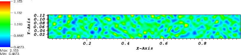
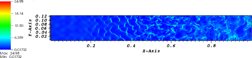
Figure 2: Plots of the distribution of the density at $t=0$ (top panel) and $t=0.04$ (bottom panel).

Figure 2 contains a plot of the distribution of the density in Simulation 4 at $t=0$ and at $t=0.04$. The fluid enters at $x=0$ and, as it is decelerated by the cosmic ray pressure, the density inhomogeneities are amplified as the regions of high density are compressed. Vorticity is generated as the regions of low density are decelerated to a greater degree than regions of high density. This creates shocks at the front of the high density regions.

Ultimately, by the time the fluid has reached $x=1$, the flow has become quite disordered and appears turbulent. We will only focus on the magnetic field amplification as this is the topic of this paper. A general study of turbulence driven in this manner would be interesting, but beyond the scope of this work.

It is clear from Figure 1 that the magnetic field is strongly amplified by the vorticity generated in the fluid by the action of the cosmic ray pressure. At the highest resolution amplification of a factor of around 20 is achieved. This gives an average magnetic field amplification in the pre-shock region, which is the diffusion scale of the highest energy cosmic rays, of around 10. Recalling that this is a lower limit (see Sect. 4) it is clear that this instability is certainly capable of amplifying the ISM magnetic field up to levels which match observations: taking an initial field of 5 $\mu$G and amplifying this to around 50 $\mu$G through this instability, and then passing it through the (strong) supernova blastwave will amplify it to around 200 $\mu$G which is in the range required to explain the observed morphology of the X-ray synchrotron emission [24, 7, 2, 3, 25, 1, 20, 23, 22, 27].

5.1 Dependence on RMS density fluctuations

Using Simulations 4 and 5 we briefly investigate the influence of varying $(\delta\rho)_{\rm rms}$, increasing it from $0.2$ to $0.44$. Figure 3 contains plots of the magnetic field amplification as a function of $x$ for each simulation. In the early stages of the development of the instability (i.e. for small $x$) the magnetic field is amplified more rapidly for higher $(\delta rho)_{\rm rms}$, as might be expected. However, as the fluid progresses towards $x=1$ the magnetic field becomes amplified to approximately the same extent in each case. This can be understood through noting that once the nonlinear effects become important (i.e. once the density inhomogeneities are significantly amplified), the overall level of turbulence and vorticity induced in the flow are approximately equal, thus leading to a similar level of magnetic field amplification.

Figure 3: Plots of the average magnetic field amplification as a function of $x$ for Simulations 4 and 5.

Of course, one does expect that as $(\delta\rho)_{\rm rms}$ increases the field amplification will also increase. It appears, though, that nonlinear effects give rise to a relatively weak dependence of field amplification on $(\delta\rho)_{\rm rms}$, at least if equations 3 and 13 are satisfied.

5.2 Dependence on initial magnetic field strength

Figure 4: As Figure 3 but for Simulations 4 and 6.

Figure 4 contains plots of the magnetic field amplification as a function of $x$ for Simulations 4 and 6. There is virtually no dependence of the magnetic field amplification on the initial field strength. Again, this is dependent on equations 3 and 13 being satisfied. However, we can conclude that for conditions appropriate to supernova blastwaves, the specific value of the magnetic field in the ISM is not important in determining the final magnetic field amplification, at least at the resolutions investigated here.

The energy density in the amplified magnetic field at $x=1$ is about 3% of that available in the velocity variations, $\delta u$, according to equation 4. One would expect then that the back-reaction of the magnetic field on the turbulent flow would be negligible and thus the specific magnetic field strength should not be important when determining the final amplification value.

6 Conclusions

We have demonstrated using a simple, but physically motivated and not unrealistic, model that significant magnetic field amplification can occur in cosmic-ray shock precursors driven by the differential acceleration of density inhomogeneities and the resultant turbulent vorticity field. A more detailed model of the diffusion of cosmic rays into the precursor would probably lead to even higher amplification because the effective diffusion would be smaller in the amplified dense knots leading to larger pressure gradients.

A noteworthy feature of the mechanism proposed here is that it operates up to what is essentially the largest scale available for any cosmic-ray driven process, the length scale of the precursor itself. Clearly no cosmic-ray driven process can operate further ahead of the shock than the length scale determined by the diffusion of the most energetic particles. It also has the great advantage of operating on scales large compared to the gyro-radius of the driving particles (at least in non-relativistic shocks where even in the Bohm limit the precursor length scale exceeds the gyro-radius by a factor of $c/U$, the ratio of the speed of light to the shock speed and typically several hundred to a thousand for SNR shocks) so that the amplified field can reduce the gyro-radius and trigger a boot-strap process. Of course other processes are possible and may add to the field amplification, particularly on smaller scales where plasma kinetic effects such as those considered by Bell can operate. The point we want to make here is simply that independent of all the detailed plasma physics, as long as there is a cosmic-ray precursor with a significant associated pressure gradient, and as long as the inflowing medium is clumpy, a well-stirred and significantly amplified magnetic field can easily be created in the precursor on the scales required.

References

- [1] J. Ballet “X-ray synchrotron emission from supernova remnants” In Advances in Space Research 37, 2006, pp. 1902–1908 DOI: 10.1016/j.asr.2005.03.047
- [2] A. Bamba, M. Ueno, H. Nakajima and K. Koyama “Thermal and Nonthermal X-Rays from the Large Magellanic Cloud Superbubble 30 Doradus C” In ApJ 602, 2004, pp. 257–263 DOI: 10.1086/380957
- [3] A. Bamba et al. “A Spatial and Spectral Study of Nonthermal Filaments in Historical Supernova Remnants: Observational Results with Chandra” In ApJ 621, 2005, pp. 793–802 DOI: 10.1086/427620
- [4] M. C. Begelman and E. G. Zweibel “Acoustic instability driven by cosmic-ray streaming” In ApJ 431, 1994, pp. 689–704 DOI: 10.1086/174519
- [5] A. R. Bell “Turbulent amplification of magnetic field and diffusive shock acceleration of cosmic rays” In MNRAS 353, 2004, pp. 550–558 DOI: 10.1111/j.1365-2966.2004.08097.x
- [6] A. Beresnyak, T. W. Jones and A. Lazarian “Turbulence-Induced Magnetic Fields and Structure of Cosmic Ray Modified Shocks” In ApJ 707, 2009, pp. 1541–1549 DOI: 10.1088/0004-637X/707/2/1541
- [7] E. G. Berezhko, L. T. Ksenofontov and H. J. Völk “Confirmation of strong magnetic field amplification and nuclear cosmic ray acceleration in SN 1006” In A&A 412, 2003, pp. L11–L14 DOI: 10.1051/0004-6361:20031667
- [8] R. Cowsik and S. Sarkar “A lower limit to the magnetic field in Cassiopeia-A” In MNRAS 191, 1980, pp. 855–861
- [9] A. Dedner et al. “Hyperbolic Divergence Cleaning for the MHD Equations” In Journal of Computational Physics 175, 2002, pp. 645–673 DOI: 10.1006/jcph.2001.6961
- [10] P. H. Diamond and M. A. Malkov “Dynamics of Mesoscale Magnetic Field in Diffusive Shock Acceleration” In ApJ 654, 2007, pp. 252–266 DOI: 10.1086/508857
- [11] L. O. Drury and S. A. E. G. Falle “On the Stability of Shocks Modified by Particle Acceleration” In MNRAS 223, 1986, pp. 353
- [12] J. Giacalone and J. R. Jokipii “Magnetic Field Amplification by Shocks in Turbulent Fluids” In ApJ 663, 2007, pp. L41–L44 DOI: 10.1086/519994
- [13] F. Guo et al. “On the Amplification of Magnetic Field by a Supernova Blast Shock Wave in a Turbulent Medium” In ApJ 747, 2012, pp. 98 DOI: 10.1088/0004-637X/747/2/98
- [14] F. Hoyle “Radio-source problems” In MNRAS 120, 1960, pp. 338–+
- [15] P. O. Lagage and C. J. Cesarsky “The maximum energy of cosmic rays accelerated by supernova shocks” In A&A 125, 1983, pp. 249–257
- [16] M. A. Malkov “Asymptotic Particle Spectra and Plasma Flows at Strong Shocks” In ApJ 511, 1999, pp. L53–L56 DOI: 10.1086/311825
- [17] M. A. Malkov and P. H. Diamond “Nonlinear Dynamics of Acoustic Instability in a Cosmic Ray Shock Precursor and its Impact on Particle Acceleration” In ApJ 692, 2009, pp. 1571–1581 DOI: 10.1088/0004-637X/692/2/1571
- [18] S. O’Sullivan and T. P. Downes “An explicit scheme for multifluid magnetohydrodynamics” In MNRAS 366, 2006, pp. 1329–1336 DOI: 10.1111/j.1365-2966.2005.09898.x
- [19] S. O’Sullivan and T. P. Downes “A three-dimensional numerical method for modelling weakly ionized plasmas” In MNRAS 376, 2007, pp. 1648–1658 DOI: 10.1111/j.1365-2966.2007.11429.x
- [20] E. Parizot, A. Marcowith, J. Ballet and Y. A. Gallant “Observational constraints on energetic particle diffusion in young supernovae remnants: amplified magnetic field and maximum energy” In A&A 453, 2006, pp. 387–395 DOI: 10.1051/0004-6361:20064985
- [21] D. Ryu, H. Kang and T. W. Jones “The stability of cosmic-ray-dominated shocks - A secondary instability” In ApJ 405, 1993, pp. 199–206 DOI: 10.1086/172353
- [22] Y. Uchiyama et al. “Extremely fast acceleration of cosmic rays in a supernova remnant” In Nature 449, 2007, pp. 576–578 DOI: 10.1038/nature06210
- [23] J. Vink “Supernova remnants: the X-ray perspective” In A&A Rev. 20, 2012, pp. 49 DOI: 10.1007/s00159-011-0049-1
- [24] J. Vink and J. M. Laming “On the Magnetic Fields and Particle Acceleration in Cassiopeia A” In ApJ 584, 2003, pp. 758–769 DOI: 10.1086/345832
- [25] H. J. Völk, E. G. Berezhko and L. T. Ksenofontov “Magnetic field amplification in Tycho and other shell-type supernova remnants” In A&A 433, 2005, pp. 229–240 DOI: 10.1051/0004-6361:20042015
- [26] G. M. Webb, A. Zakharian and G. P. Zank “Wave mixing and instabilities in cosmic-ray-modified shocks and flows” In Journal of Plasma Physics 61, 1999, pp. 553–599 DOI: 10.1017/S0022377898007466
- [27] R. Yamazaki et al. “Constraints on the diffusive shock acceleration from the nonthermal X-ray thin shells in SN 1006 NE rim .” In A&A 416, 2004, pp. 595–602 DOI: 10.1051/0004-6361:20034212