LMM-Lasso: A Lasso Multi-Marker Mixed Model for Association Mapping with Population Structure Correction

Abstract

1 Motivation:

Exploring the genetic basis of heritable traits remains one of the central challenges in biomedical research. In traits with simple mendelian architectures, single polymorphic loci explain a significant fraction of the phenotypic variability. However, many traits of interest appear to be subject to multifactorial control by groups of genetic loci. Accurate detection of such multivariate associations is non-trivial and often compromised by limited power. At the same time, confounding influences such as population structure cause spurious association signals that result in false positive findings if they are not accounted for in the model.

2 Results:

We propose LMM-Lasso, a mixed model that allows for both multi-locus mapping and correction for confounding effects. Our approach is simple and free of tuning parameters, effectively controls for population structure and scales to genome-wide datasets. LMM-Lasso simultaneously discovers likely causal variants and allows for multi-marker based phenotype prediction from genotype. We demonstrate the practical use of LMM-Lasso in genome-wide association studies in Arabidopsis thaliana and linkage mapping in mouse, where our method achieves significantly more accurate phenotype prediction for $91\%$ of the considered phenotypes. At the same time, our model dissects the phenotypic variability into components that result from individual SNP effects and population structure. Enrichment of known candidate genes suggests that the individual associations retrieved by LMM-Lasso are likely to be genuine.

3 Availability:

Code available under XXX.

4 Contact:

{rakitsch, clippert, stegle}@tuebingen.mpg.de {rakitsch, clippert, stegle}@tuebingen.mpg.de

5 Introduction

While many quantitative traits in humans, plants and animals have been observed to be heritable, a comprehensive understanding of the underlying genetic architecture is still missing. In some cases genome-wide association studies and linkage mapping have already revealed individual causal variants that control trait variability; for example, genetic mapping yielded insights into the genetic architecture of global-level traits in plants Atwell2010 and mouse valdar2006genome , as well as the risks for important human diseases such as type 2 diabetes craddock2010genome . Nevertheless, the statistical analysis of these genetic data has proven to be challenging, not least because single genetic variants rarely explain larger fractions of phenotype variability, and hence, individual effect sizes are small mccarthy2008genome ; mackay_genetics_2009 . An inherent limitation of power to map weak effects is due to confounding relatedness between samples. Population structure can induce false association patterns with large numbers of loci being correlated with the phenotype. To understand the true genetic architecture of complex traits, it is necessary to address both of these challenges, taking population structure into account and joint modeling of true multifactorial associations.

If multiple variants contribute to phenotype variation in an additive fashion, simple methods that assess the significance of individual loci independently are likely to fall short: masking effects between causal SNPs can limit mapping power, with relevant loci not reaching genome-wide significance levels mccarthy2008genome . These shortcomings have been widely addressed in multivariate regression, explicitly modeling the additive effect of multiple SNPs.

The corresponding methods either fit sparse predictors of all genome-wide SNPs, using a shrinkage prior or employ stepwise forward selection yang2012conditional . Applying a Laplace prior leads to the Lasso li2011bayesian , and related priors have also been considered balding-2008-1 . With the same ultimate goal to capture the genetic effects of groups of SNPs, variance component models have recently been proposed to quantify the heritable component of phenotype variation explainable by an excess of weak effects visscher-2010-1 .

Population structure induces spurious correlations between genotype and phenotype, complicating the genetic analysis. A major source of these effects can be understood as deviation from the idealized assumption that the samples in the study population are unrelated. Instead, population structure in the sample is difficult to avoid and even in a seemingly stratified sample, the extent of hidden structure cannot be ignored newman2001importance . Models that account for the presence of such structure are routinely applied and have been shown to greatly reduce the impact of this confounding source of variability. For instance, EIGENSTRAT builds on the idea of extracting the major axes of population differentiation using a PCA decomposition of the genotype data price2006principal , and subsequently including them into the model as additional covariates. Linear mixed models yu2006unified ; kang2008efficient ; zhang2010 ; Kang2010 ; fastlmm provide for more fine-grained control by modeling the contribution of population structure as a random effect, providing for an effective correction of family structure and cryptic relatedness.

While both, correction for population structure and joint mapping of multiple weak effects, have been addressed in isolation, few existing approaches are capable of addressing both aspects jointly. In line with EIGENSTRAT, the authors of balding-2008-1 ; li2011bayesian add principal components to the model to correct for population structure. In parallel to our work, Segura et. al bjarni2012 have proposed a related multi-locus mixed model approach, however employing step-wise forward selection instead of using the Lasso.

Here, we propose a novel analysis approach that combines multivariate association analysis with accurate correction for population structure. Our method allows for joint identification of sets of loci that individually have small effects and at the same time accounts for possible structure between samples. This joint modeling explains larger fractions of the total phenotype variability while dissecting it in variance components specific to individual SNP effects and population effects.

Our approach bridges the advantages of linear mixed models with Lasso regression, hence, modeling complex genetic effects while controlling for relatedness in a comprehensive fashion. The proposed LMM-Lasso is conceptually simple, computationally efficient and scales to genome-wide settings. Experiments on semi-empirical data show that the rigorous combination of Lasso and mixed modeling approaches yields greater power to detect true causal effects in a large range of settings. In retrospective analyses of studies from Arabidopsis and mouse, we show that through joint modeling of population structure and individual SNP effects, LMM-Lasso results in superior models of the genotype to phenotype map. These yield better quantitative predictions of phenotypes while selecting only a moderate number of SNP with individual effects. Additional evidence of the effects uncovered by LMM-Lasso likely being real is given by an enrichment analysis, suggesting that the hits obtained are often in the vicinity of genes with known implication for the phenotype.

6 Multivariate linear mixed models

Our approach builds on multivariate statistics, explaining the phenotype variability by a sum of individual genetic effects and random confounding variables. In brief, the phenotype of $m$ samples ${\bf y}=(y_{1},\ldots,y_{m})$ is expressed as the sum of $n$ SNPs ${\bf S}=(\mathbf{s}_{1},\ldots,\mathbf{s}_{n})$

$${\bf y}=\underbrace{\sum_{j=1}^{n}\beta_{j}{\bf s}_{j}}_{\text{genetic factors}}+\underbrace{{\bf u}}_{\text{confounding}}+\underbrace{\mbox{\boldmath$\psi$}}_{\text{noise}}.$$ (1)

Here, $\psi$ denotes observation noise and ${\bf u}$ are confounding influences. Confounding influences in genetic mapping are typically not directly observed, however their Gaussian covariance ${\bf K}$ can in many cases be estimated from the observed data. To account for confounding by population structure, ${\bf K}$ can be reliably estimated from genetic markers, for example using the realized relationship matrix which captures the overall genetic similarity between all pairs of samples hayes-2009-1 . Similarly, in genetic analyses of gene expression, ${\bf K}$ can be fit to capture and correct for the confounding effect of gene expression heterogeneity listgarten2010correction ; fusi2012joint . Marginalizing over the random effect ${\bf u}$ results in a Gaussian marginal likelihood model kang2008efficient whose covariance matrix accounts for confounding variation and observation noise.

The resulting mixed model is typically considered in the context of single candidate SNPs, i.e. restricting the sum in Eq. (1) to a particular SNP while ignoring all others yu2006unified ; kang2008efficient ; zhang2010 ; Kang2010 ; fastlmm . While computationally efficient and easy to interpret, this independent analysis can be compromised by complex genetic architectures with some genetic factors masking others platt2010conditions . Some improvement can be achieved by step-wise regression or forward selection, which has recently been extended to the mixed model framework yang2012conditional ; bjarni2012 . However as any step-wise procedure in general, these approaches are prone to retrieving local optima as the order in which SNP markers are added matters. As an alternative, we propose an efficient approach to carry out joint inference in the model implied by Eq. (1). Our approach assesses all SNPs at the same time while accounting for their interdependencies and without making any assumptions on their ordering. To allow for applications to genome-wide SNP data, we place a Laplacian shrinkage prior over the fixed effects $\beta_{i}$, assigning zero effect size to the majority of SNPs as done in the classical Lasso tibshirani-1996-lasso .

We call this approach LMM-Lasso as it combines the advantages of established linear mixed models (LMM) with sparse Lasso regression. The resulting model allows for dissecting the explained phenotype variance into a component due to individual SNP effects and effects caused by confounding structure.

6.1 Linear mixed model Lasso

Let ${\bf S}$ denote the $m\times n$ matrix of $n$ SNPs for $m$ individuals, ${\bf s}_{j}$ is then the $m\times 1$ vector representing SNP $j$. We model the phenotype for $m$ individuals, ${\bf y}=(y_{1},\dots,y_{m})$ as the sum of genetic effects $\beta_{j}$ of SNPs ${\bf s}_{j}$ and confounding influences ${\bf u}$ (see Eq. (1)). The genetic effects are treated as fixed effects, whereas the confounding influences are modeled as random effects. The genetic effect terms are summed over genome-wide polymorphisms, where the great majority of SNPs has zero effect size, i.e. $\beta_{j}=0$, which is achieved by a Laplace shrinkage prior on all weights. The random variable ${\bf u}$ is not observed directly. Instead, we assume that the distribution of ${\bf u}$ is Gaussian with covariance ${\bf K}$, ${\bf u}\sim\mathcal{N}(0,\sigma_{g}^{2}{\bf K})$.

Assuming Gaussian noise, $\mbox{\boldmath$\psi$}\sim\mathcal{N}(0,\sigma_{e}^{2}{\bf I})$, and marginalizing over the random variable ${\bf u}$, we can write down the conditional posterior distribution over the weight vector $\beta$:

$$p(\mbox{\boldmath$\beta$}\,|\,{\bf y},{\bf S},{\bf K},\sigma_{g}^{2},\sigma_{e}^{2},\lambda)\propto$$

$$\;\;\;\;\;\;\;\;\;\underbrace{\mathcal{N}({\bf y}\,|\,\sum_{j=1}^{n}\beta_{j}{\bf s}_{j},\sigma_{g}^{2}{\bf K}+\sigma_{e}^{2}{\bf I})}_{\text{marginal likelihood}}\underbrace{\prod_{j=1}^{n}e^{-\frac{\lambda}{2}|\beta_{j}|_{1}}}_{\text{prior}}.$$ (2)

Here, $\lambda$ denotes the sparsity hyperparameter of the Laplace prior, $\sigma_{e}^{2}$ is the residual noise variance and $\sigma_{g}^{2}$ denotes the variance of the random effect components.

6.2 Parameter inference

Learning the hyperparameters $\mbox{\boldmath$\Theta$}=\{\lambda,\sigma_{g}^{2},\sigma_{e}^{2}\}$ and the weights $\beta$ jointly is a hard non-convex optimization problem. Here, we propose a combination of fitting some of these parameters on the null model with the individual SNP effects excluded and reduction to a standard Lasso regression problem.

Null-modell fitting

To obtain a practical and scalable algorithm, we first optimize $\sigma_{g}^{2},\sigma_{e}^{2}$ by Maximum Likelihood under the null model, ignoring the effect of individual SNPs. The analogous procedure is widely used in single-SNP mixed models, and has been shown to yield near-identical result to an exact approach (Kang2010, ). To speed up the computations needed, we optimize the ratio of the random effect and the noise variance, $\delta={\sigma_{e}^{2}}/{\sigma_{g}^{2}}$, which can be optimized efficiently by using computational tricks proposed elsewhere fastlmm :

$$p(\mbox{\boldmath$\beta$}\,|\,{\bf y},{\bf S},{\bf K},\sigma_{g}^{2},\delta,\lambda)\propto\mathcal{N}({\bf y}\,|\,\sum_{j=1}^{n}\beta_{j}{\bf s}_{j},\sigma_{g}^{2}({\bf K}+\delta{\bf I}))\prod_{j=1}^{n}e^{-\frac{\lambda}{2}|\beta_{j}|_{1}}.$$ (3)

Briefly, we compute the eigendecomposition of the covariance $\bf K={\bf U}{\rm diag}({\bf d}){\bf U}^{{\rm T}}$ which can be used to rotate the data such that the covariance matrix of the normal distribution is isotropic. We carry out one-dimensional numerical optimization of the marginal likelihood (Eq. (6.1)) with respect to $\delta$, whereas $\sigma_{g}^{2}$ can be optimized in closed form in every evaluation.

Reduction to standard Lasso problem

Having fixed $\delta$, we use the eigendecomposition of ${\bf K}$ again to rotate our data such that the covariance matrix becomes isotropic:

$$p(\mbox{\boldmath$\beta$}\,|\,\tilde{{\bf y}},\tilde{{\bf S}},{\bf K},\sigma_{g}^{2},\lambda)\propto\mathcal{N}(\tilde{\bf y}\,|\,\sum_{j=1}^{n}\beta_{j}\tilde{{\bf s}}_{j},\sigma_{g}^{2}{\bf I})\prod_{j=1}^{n}e^{-\frac{\lambda}{2}|\beta_{j}|_{1}}$$ (4)

Here, $\tilde{{\bf S}}$ denote the rotated and rescaled genotypes and $\tilde{{\bf y}}$ the respectively phenotypes:

$$\bf{\tilde{S}}=({\rm diag}({\bf d})+\delta{\bf I})^{-\frac{1}{2}}\bf{U^{T}S}, \bf{\tilde{y}}=({\rm diag}({\bf d})+\delta{\bf I})^{-\frac{1}{2}}\bf{U^{T}y}.$$

Using this transformation, the task of determining the most probable weights in Eq. (4) is now equivalent to the Lasso regression model, since maximizing the posterior with respect to $\beta$ is equivalent to minimizing the negative log of Eq. (4):

$$\min_{\mbox{\boldmath$\beta$}}\frac{1}{\sigma_{g}^{2}}||{\tilde{\bf y}}-\tilde{{\bf S}}\mbox{\boldmath$\beta$}||_{2}+\lambda\|\mbox{\boldmath$\beta$}\|_{1}.$$

A related algorithm for combining random effects with the Lasso has been proposed in schelldorfer-2011-1 , which includes a generalized linear mixed models with $\ell_{1}$-penalty at the cost of higher computational complexity. An appropriate setting of $\lambda$ can be found by cross-validation to maximize the overall predictive performance or stability selection buehlmann-ss-2010-1 .

The computational efficiency of the two-stage procedure proposed here depends on the approximation to fit $\delta$ on the null model, allowing for the reduction of the problem to standard Lasso regression. For univariate single-SNP mixed models, efficient optimization of $\delta$ for each SNP can be done by recently proposed computational tricks fastlmm ; Stephens2012 . Unfortunately, these techniques cannot be directly applied in the multivariate setting. In principle it is possible to extend the cross-validation to optimize over pairs ($\delta,\lambda$). However, this remains impracticable for most datasets due to the additional computational cost implied and hence we consider optimizing $\delta$ on the null model in the experiments Kang2010 .

6.3 Phenotype prediction

Given a trained LMM-Lasso model on a set of genotype and phenotypes, we can predict the unobserved phenotype of test individuals. The predictive distribution can be derived by conditioning the joint distribution over all individuals on the training individuals rasmussen_gaussian_2006 , resulting in a Gaussian predictive distribution $p({\bf y}^{\star}\,|\,{\bf y},{\bf S^{\star}},{\bf S})=\mathcal{N}({\bf y}^{\star}\,|\,\mbox{\boldmath$\mu$}^{\star},\mbox{\boldmath$\Sigma$}^{\star})$, with

$$\mbox{\boldmath$\mu$}^{\star} = \underbrace{{\bf S^{\star}}\mbox{\boldmath$\beta$}}_{\text{Lasso prediction}}+\underbrace{{\bf K}_{{\bf S}^{\star}{\bf S}}({\bf K}+\delta{\bf I})^{-1}({\bf y}-{\bf S}\mbox{\boldmath$\beta$})}_{\text{Random effect prediction}}$$

$$\mbox{\boldmath$\Sigma$}^{\star} = \sigma_{g}^{2}({\bf K}_{{\bf S}^{\star}{\bf S}^{\star}}+\delta{\bf I})-\sigma_{g}^{2}{\bf K}_{{\bf S}^{\star}{\bf S}}({\bf K}+\delta{\bf I})^{-1}{\bf K}_{{\bf S}{\bf S}^{\star}}.$$ (5)

The mean prediction is a sum of contributions from the Lasso component and the random effect part, which is similar to BLUP (robinson1991blup, ). The matrix ${\bf K}_{{\bf S}^{\star}{\bf S}}$ denotes the covariance matrix between the test individuals $\bf S^{\star}$ and the train individuals $\bf S$, ${\bf K}_{{\bf S}^{\star}{\bf S}^{\star}}$ is the covariance matrix between all test individuals and ${\bf K}:={\bf K}_{{\bf S}{\bf S}}$ is the covariance matrix between all training individuals, which with slight abuse of notation are denoted by their genetics ${\bf S}$.

6.4 Choice of the random effect covariance to account for population structure

Depending on the application, the random effect covariance ${\bf K}$ can be chosen in a variety of ways. Here, we discuss specific options to account for population structure.

Choice of genetic similarly matrix

For the identity by descent matrix (IBD), an entry is defined as the predicted proportion of the genome that is identical by descent given the pedigree information. In contrast, the identity by state matrix (IBS) simply counts the number of loci on which the samples agree, where as the realized relationship matrix (RRM) is calculated as the linear kernel between the SNPs hayes-2009-1 . In subsequent experiments, we have used the realized relationship matrix. An example for the RRM-matrix derived from the Arabidopsis thaliana dataset is given in Figure S1.

Realized relationship matrix and relationship to Bayesian linear regression

From a Bayesian perspective, employing the realized relationship matrix as the covariance matrix is equivalent to integrating over all SNPs in a linear additive model with an independent Gaussian prior over the weights $\mathcal{N}(\mbox{\boldmath$\beta$}\,|\,{\bf{0}},\sigma_{g}^{2}{\bf I})$  goddard_2009-1 . The choice of a Gaussian prior leads to a dense posterior distribution, reflecting the a priori belief that a large fraction of SNPs jointly contribute to phenotype variability. This prior choice is in sharp contrast to the generally accepted opinion that most SNPs are not causal.

Thus, choosing this particular covariance matrix $\bf K$ can be regarded as modeling genetic effects that are confounded due to population structure or are small additive infinitesimal effects, whereas single SNPs that have a sufficiently large effect size are directly included in the Lasso of model.

6.5 Scalability and runtime

The appeal of the LMM-Lasso is a runtime performance comparable the standard LASSO. The difference is a one-time off cubic cost for the decomposition of the random effect matrix ${\bf K}$ to rotate the genotype and phenotype data (see Section 6.2).

To demonstrate the applicability to genome-wide datasets, we have empirically measured the runtime for computing the complete path of sparsity regularizers on the synthetic dataset, consisting of 1,196 plants and 213,624 SNPs. On a single core of a Mac Pro (3GHz, 12 MB L2-Cache, 16GB Memory), the Lasso required 145 minutes CPU time and the LMM-Lasso 146 minutes of CPU time.

If needed, the runtime of LMM-Lasso could be improved in several ways. First, if the number of samples is large (m $>10^{5}$), the runtime is dominated by the decomposition of ${\bf K}$ and rotating the data for the optimization of $\delta$. As shown in fastlmm , reducing the covariance ${\bf K}$ to a low-rank representation calculated from a small subset of $n_{s}$ SNPs, yields very similar results while reducing the runtime from $O(m^{2}n)$ to $O(mn_{s}^{2})$. Second, the runtime of the $\ell_{1}$-solver is heavily dependent on the optimization method used. Fortunately, the development of new and efficient $\ell_{1}$-solvers is still an active area of research. New approaches include parallelized coordinate descent algorithms bradley2011 and screening tests that are able to prune away SNPs that are guaranteed to have zero weights xiang-2011-1 , avoiding to load the complete genotype matrix into the working memory.

7 Methods and Material

7.1 Arabidopsis thaliana

We obtained genotype and phenotype data for up to 199 accessions of Arabidopsis thaliana from Atwell2010 . Each genotype comprises 216,130 single nucleotide polymorphisms per accession. We study the group of phenotypes related to the flowering time of the plants. We excluded phenotypes that were measured for less than 150 accessions to avoid possible small sample size effects, resulting in a total of 20 flowering phenotypes that were considered. The relatedness between individuals ranges in a wide spectrum leading to a complex population structure platt-2010-1 .

7.2 Mouse inbred population

We also obtained genotype and phenotype data for 1,940 mice from a multi-parent inbred population valdar2006genome . Each individual genotype comprises of 12,226 single nucleotide polymorphisms. All mice were derived from eight inbred strains and were crossed to produce a heterogenous stock. The phenotypes span a large variety of different measurements ranging from biochemical to behavioral traits. Here, we focused on 273 phenotypes which have numeric or binary values.

7.3 Semi-empirical data

To assess the accuracy of alternative methods for variable selection, we considered a semi-empirical example based on the extended A. thaliana dataset bergelson-2012-1 consisting of 1196 plants. We considered real phenotype data to obtain realistic background signal that is subject to population structure. In addition to this empirical background, we added simulated associations with different effect sizes and a range of complexities of the genetic models. For full details of the simulation procedure and the evaluation of associations recovered by different methods, see supplementary text.

7.4 Preprocessing

We standardized the SNP data which has the effect that SNPs with a smaller MAF have a larger effect size as reported in amos_shifting_2008-1 . On the phenotypes, we performed a Box-Cox transformation saskia_boxcox-1992-1 and subsequently standardized the data.

7.5 Model Selection

Variation of the model complexity of Lasso Methods can either be done by choosing the number of active SNPs or equivalently by varying the hyperparameter $\lambda$ explicitly. For the benefit of direct interpretability, we chose to vary the number of active SNPs. For a fixed number of selected SNPs, we find the corresponding hyperparameter $\lambda$ by a combination of bracketing and bisection as done in wu_gwaslars-2009-1 .

To select which of these Lasso-model is most suitable, we consider alternative strategies, depending on the objective.

1. Phenotype prediction To predict phenotypes, we use 10-fold cross-validation. We split the data randomly into 10 folds. Each fold is once picked as test dataset, with all other folds being used for training the model. The model is selected to maximize the explained variance on the test set. In this comparison, we considered models with different numbers of SNPs, varying from $\{0,1,2,\ldots,10,20,30,\ldots,100,150,200,250\}$ with the additional constraint that the number of active SNPs shall not exceed the number of samples.

2. Variable selection To assess the significance of individual features, we consider stability Selection buehlmann-ss-2010-1 . Here, we fix the number of active SNPs to $20$ and draw randomly $90\%$ of the data $100$ times. Significance estimates can be deduced from the selection frequency of individual SNPs (see buehlmann-ss-2010-1 ).

   To obtain a complete ranking of features, as used to evaluate models in the simulation study, we use the LASSO regularization path and rank features by the order of inclusion into the model.

8 Results

8.1 Semi-empirical setting with known ground truth

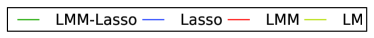
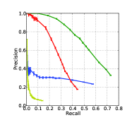
(a)

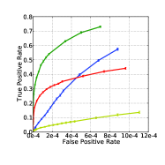
(b)

Figure 1: Evaluation of alternative methods on semi-empirical GWAS datasets, mimicking population structure as found in Arabidopsis thaliana. (a) Precision-Recall Curve for recovering simulated causal SNPs using alternative methods. Shown is precision (TP/(TP+FP)) as a function of the recall (TP/(TP+FN)). (b) Alternative evaluation of each method on the identical dataset using Receiver operating characteristics (ROC). Shown is the True Positive Rate (TPR) as a function of the False Positive Rate (FPR).

We assessed the ability of LMM-Lasso to recover true genotype to phenotype associations in a semi-empirical simulated dataset. To ensure realistic characteristics of population structure, we simulated confounding such that it borrows key characteristics from Arabidopsis thaliana, a strongly structured population.

To compare our method to existing techniques, we considered the standard Lasso, which models all SNPs jointly but without correcting for population structure, as well as univariate Linear Mixed Models, which effectively control for confounding, but consider each SNP in isolation. As a baseline, we also considered a standard univariate Linear Model (LM), which neither accounts for confounding nor considers joint effects due to complex genetic architectures. Both, the standard Lasso and LMM-Lasso were fit in identical ways (See Section 7.5). For the linear mixed model and the LMM-Lasso, we used the RRM as covariance matrix and fit $\delta$ on the null model. For univariate models, the ranking of individual SNPs was done according to their p-values, for multivariate models we considered the order of inclusion into the model. A fair comparison between the univariate and multivariate methods is difficult as the univariate methods select blocks of linked markers, whereas the multivariate methods select only one representative marker per block (see Supplementary text S1, Section 1).

LMM-Lasso ranks causal SNPs higher than alternative methods

(a)

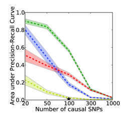
(b)

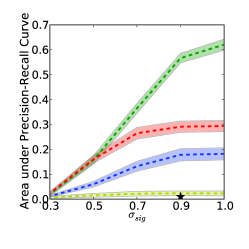
(c)

Figure 2: Evaluation of alternative methods on the semi-empirical GWAS dataset for different simulation settings. Area under precision recall curve for finding the true simulated associations. Alternative simulation parameters have been varied in a chosen range. (a) Evaluation for different relative strength of population structure $\sigma_{\text{pop}}$. (b) Evaluation for true simulated genetic models with increasing complexity (more causal SNPs). (c) Evaluation for variable signal to noise ratio $\sigma_{\text{sig}}$.

First, we compared the alternative methods in terms of their accuracy in recovering SNPs with a true simulated association (Figure 1a). Methods that account for population structure (LMM-Lasso, LMM) are more accurate than their counter parts, with LMM-Lasso performing best. While the linear mixed model performs well at recovering strong associations, the independent statistical testing falls short in detecting weaker associations which are likely masked by stronger effects (Figure S2a). Comparing methods that account for population structure and naive methods, we observe that accounting for this confounding effect avoids the selection of SNPs that merely reflect relatedness without a causal effect (Figure S2b). An alternative evaluation, which considers the receiver operating characteristic curve, given in Figure 1b, yields identical conclusions.

Next, we explored the impact of variable simulation settings. As common in the literature, we used the area under the precision-recall curve as a summary performance measure to compare different algorithms. Precision and recall both depend on the decision threshold, above which a marker is predicted to be activated. By varying this threshold, one obtains a precision-recall curve. Figure 2a shows the area under the precision recall curve as a function of an increasing ratio of population structure and independent environmental noise. When the confounding population structure is weak, both the Lasso and the LMM-Lasso perform similar. As expected, the benefits of population structure correction in LMM-Lasso are most pronounced in the regime of strong confounding.

We also examined the ability of each method to recover genetic effects for increasing complexities of the genetic model, varying the number of true causal SNPs while keeping the overall genetic heritability fixed (Figure 2b). LMM-Lasso performs better than alternative methods for the whole range of considered settings with the difference in accuracy being the largest for genetic architectures of medium complexity. In a nutshell, these results show that, in the regime of a larger number of true weak associations, it is advantageous to include a genetic covariance ${\bf K}$ that accounts for some of the weak effects visscher-2010-1 .

The identical effect is observed when varying the ratio between true genetic signal versus confounding and noise (Figure 2c). Again, the performance of the LMM-Lasso is superior to all other methods and the strengths are particularly visible for medium signal to noise ratios.

8.2 LMM-Lasso explains the genetic architecture of complex traits in model systems

Having shown the accuracy of LMM-Lasso in recovering causal SNPs in simulations, we now demonstrate that the LMM-Lasso better models the genotype-to-phenotype map in Arabidopsis thaliana and mouse valdar2006genome . Here, we focus on 20 flowering time phenotypes for Arabidopsis thaliana, which are well characterized, and 273 mouse phenotypes which are relevant to human health.

LMM-Lasso more accurately predicts phenotype from genotype and uncovers sparser genetic models

(a)

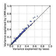
(b)

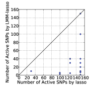
(c)

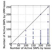
(d)

Figure 3: Predictive power and sparsity of the fitted genetic models for Lasso and LMM-Lasso applied to quantitative traits in model systems. Considered were flowering phenotypes in Arabidopsis thaliana and bio-chemical and physiological phenotypes with relevance for human health profiled in mouse. Comparative evaluations include the fraction of the phenotypic variance predicted and the complexity of the fitted genetic model (number of active SNPs). (a) Explained variance in Arabidopsis. (b) Explained variance in mouse. (c) Complexity of fitted models in Arabidopsis. (d) Complexity of fitted models in mouse.

First, we considered phenotype prediction to investigate the capability of alternative methods to explain the joint effect of groups of SNPs on phenotypes. To measure for the predictive power, we assessed which fraction of the total phenotypic variation can be explained by genotype using different methods henner-dros-2012-1 . Explained variance is defined as the fraction of the total variance of the phenotype that can be explained by the model and in our experiments equals one minus the mean squared error as we preprocesed the data to have zero-mean and unit-variance. We avoided prediction on the training data, as for all methods this leads to anti-conservative estimates of variance explained due to overfitting (see Figure S 4 for a comparison).

Figure 3a and 3b show the explained variance of the two methods on the independent test data set for each phenotype in the two datasets. For both model organisms, LMM-Lasso explained at least as much variation as the Lasso. We omitted the univariate methods, as their performance is generally lower due to the simplistic assumption of a single causal SNP (See Figure S4 for comparative predictions in Arabidopsis thaliana). In a fraction of $85.00\%$ of the Arabidopsis thaliana and $91.58\%$ of the mouse phenotypes, LMM-Lasso was more accurate in predicting the phenotype and thus explained a greater fraction of the phenotype variability from genetic factors than the Lasso. In contrast, Lasso achieved better performance in only $15\%$ of the Arabidopsis thaliana and $8.42\%$ of the mouse phenotypes. Beyond an assessment of the genetic component of phenotypes, LMM-Lasso dissects the phenotypic variability into the contributions of individual SNPs and of population structure. Figure 3c and 3d show the number of SNPs selected in the respective genetic models for prediction. With the exception of two phenotypes, LMM-Lasso selected substantially fewer SNPs than the Lasso, suggesting that the Lasso includes additional SNPs into the model to capture the effect of population structure through an additional set of individual SNPs. This observation is in line with the insights derived from the simulation setting where the majority of excess SNPs selected by Lasso are indeed driven by population effects (S 2b). Although the genetic models fit by LMM-Lasso are substantially sparser, they nevertheless suggest complex genetic control by multiple loci. In $90.00\%$ of Arabidopsis thaliana and in $66.06\%$ of the mouse phenotypes, LMM-Lasso selected more than one SNP, in $40.00/45.49\%$ of the cases the number of SNPs in the model was greater than $10$.

LMM-Lasso allows for dissecting individual SNP effects from global genetic effects driven by population structure

Figure 4: Variance dissection into individual SNP effects and global genetic background driven by population structure. Shown is the explained variance on an independent test set as a function of the number of active SNPs for the flowering phenotype ($10^{\circ}$) in Arabidopsis thaliana. In blue, the predictive test set variance of the Lasso as a function of the number of SNPs in the model. In green, the total predictive variance of LMM-Lasso for different sparsity levels. The shaded area indicates the fraction of variance LMM-Lasso explains by means of population structure (yellow) and population structure (green). LMM-Lasso without additional SNPs in the model corresponds to a genetic random effect model (black star).

Next, we investigated the ability of LMM-Lasso to differentiate between individual genetic effects and effects caused by population structure. Figure 4 shows the explained variances for the phenotype flowering time (measured at $10^{\circ}C$) for Arabidopsis thaliana. Again, these estimates were obtained using a cross validation approach. It is known zhao_as-2007-1 that flowering is strikingly associated with population structure, which explains why the LMM-Lasso already captured a substantial fraction ($45.17\%$) of the phenotypic variance, when using realized relationships alone (number of active SNPs=0). Due to the small sample size, cross-validation can underestimate the true explained variance hastie_esl-2003-1 . Nevertheless, cross-validation is fair for comparison and conservative as it avoids possible overfitting.

For increasing number of SNPs included in the model, the explained variance of LMM-Lasso gradually shifted from the kernel to the effects of individual SNPs. In this example the best performance ($48.87\%$) was reached with 30 SNPs in the model where the relative contribution of the random effect model was $33.10\%$ and of the individual SNPs is $15.77\%$. In comparison, Lasso explained at most $46.53\%$ of the total variance, when 125 SNPs were included in the model.

Associations found by LMM-Lasso are enriched for SNPs in proximity to known candidate genes

Phenotype	LMM-Lasso	Lasso
LD	5/54	4/69
LDV	5/63	3/69
SD	3/55	2/61
SDV	5/54	2/60
FT10	1/48	4/67
FT16	3/51	4/68
FT22	2/54	1/64
2W	3/53	2/65
8W	2/51	4/59
FLC	5/52	3/53
FRI	3/43	3/46
8WGHFT	4/59	2/66
8WGHLN	1/48	4/58
0WGHFT	4/58	3/63
FTField	4/61	3/69
FTDiameterField	1/49	1/51
FTGH	1/49	2/61
LN10	3/50	2/67
LN16	2/58	3/64
LN22	4/54	2/65

Table 1: Associations close to known candidate genes. We report true positives/positives (TP/P) for LMM-Lasso and Lasso for all phenotypes related to flowering time in Arabidopsis thaliana. P are all activated SNPs and TP are all activated SNPs that are close to candidate genes.

Finally, we considered the associations retrieved by alternative methods in terms of their enrichment near candidate genes with known implications for flowering in Arabidopsis thaliana. It can be advantageous to remove the SNP of interest from the population structure covariance (see also discussion in fastlmm ). Thus, we applied LMM-Lasso on a per-chromosome basis estimating the effect of population structure from all remaining chromosomes. To obtain a comparable cutoff of significance, we employed stability selection for both the LMM-Lasso and Lasso (See Section 7.5).

Table 1 shows that the LMM-Lasso found a greater number of SNPs linked to candidate genes for twelve phenotypes, whereas Lasso retrieved a greater number for only six phenotypes. In the remaining two phenotypes, both methods performed identically (For a complete list of candidate genes found by LMM-Lasso, See Table S1). It is difficult to compare the multivariate approaches with univariate techniques in a quantitative manner since the univariate models tend to retrieve complete LD-Blocks. Thus, we revert to reporting the p-values of the univariate methods for the SNPs detected by the LMM-Lasso.

We also considered to what extent the findings yield evidence for genetic heterogeneity in proximity to candidate genes (as in the simulated setting in Figure 3). Overall, $14.75\%$ of the SNPs linked to candidate genes and selected by the LMM-Lasso appear as adjacent pairs (Table S2), i.e. having a distance less than 10kb to each other, while $5.56\%$ of the SNPs selected by the Lasso do. From all activated SNPs, $8.18\%$ selected by LMM-Lasso and $18.96\%$ selected by the Lasso have at least a second active SNP in close proximity. A simulated example, illustrating how the LMM-Lasso can detect genetic heterogeneity is shown in Supplementary text S1, Section 3.

9 Discussion

Here, we have presented a Lasso multi-marker mixed model (LMM-Lasso) for detecting genetic associations in the presence of confounding influences such as population structure. The approach combines the attractive properties of mixed models that allow for elegant correction for confounding effects and those of multi-marker models that consider the joint effects of sets of genetic markers rather than one single locus. As a result, LMM-Lasso is able to better recover true genetic effects, even in challenging settings with complex genetic architectures, weak effects of individual markers or presence of strong confounding effects.

LMM-Lasso is relevant for genome-wide association studies of complex phenotypes, particularly the large number of phenotypes whose genetic basis is conjectured to be multifactorial flint-2009-1 . Here, we have demonstrated such practical use through retrospective analysis of Arabidopsis thaliana and data from inbred mouse lines. First, we found that the combination of random effect modeling and multivariate linear models as done in LMM-Lasso improves the prediction of phenotype from genotype, suggesting that the underlying model that accounts for both, population structure effects and multi-locus effects, is a better fit to real genetic architectures. It is widely accepted that the missing heritability in single-locus genome wide association mapping can often be explained by a large number of loci that have a joint effect on the phenotype visscher-2010-1 while leading only to weak signals of association if considered independently. In addition to recovering greater fractions of the heritable component of quantitative traits, LMM-Lasso allows for differentiating between variation that is broad-scale genetic and hence likely caused by population structure and individual genetic effects. In Arabidopsis and mouse, this approach revealed substantially sparser genetic models than naive Lasso approaches. Second, LMM-Lasso retrieves genetic associations that are enriched for known candidate genes. In line with the findings in yang2012conditional , we retrieved an increased rate of physically adjacent SNPs selected in proximity to candidate genes.

Neither the concept of accounting for population structure nor multivariate modeling of the genetic data are novel per se. An approach for distincting populations based on multi-task learning is presented in  xing-2010-1 . There is a vast amount of literature using a $\ell_{1}$-regularized approach for genome-wide associations studies wu_gwaslars-2009-1 ; xing-2012 ; kim2009 . In foster-2007-1 , as sparse random effect model is proposed, where the markers are modeled as random Lasso effects. In  balding-2008-1 ; li2011bayesian , the authors suggest to add principal components to the model to correct for population structure. While these approaches can be effective in some settings, principal components cannot account for family structure or cryptic relatedness price2010 . Importantly, none of these approaches considers including random effects to control for confounding. A notable exception is the general L1 mixed model framework by Schelldorfer et. al. schelldorfer-2011-1 , who consider a random effect component but do not provide a scalable algorithm that is applicable to genome-wide settings.

The proposed model is also closely related to existing mixed models, however these are predominantly considering individual SNPs in isolation. An exception is work in parallel bjarni2012 who propose a joint model of multiple large effect loci in a mixed model using a step-wise regression approach. An important difference to our work is the sequential selection of SNPs, which implies an effect due to ordering whereas LMM-Lasso selects all SNPs jointly.

As sample sizes increase, the power of detecting multifactorial effects will quickly rise. Moreover, larger datasets improve the feasibility to estimate accurate p-values of individual markers by using stability selection meinshausen-2009-1 , which involves randomized splitting of the dataset. However, it is unclear how strongly the sample size splitting affects the power of Lasso-based methods. Our results suggest that $\ell_{1}$-regularized methods can indeed be an attractive tool for fitting multifactorial effects in genetic settings, however assessing the statistical significance without loosing power remains a challenge for future research for Lasso methods in general.

LMM-Lasso addresses the problem that multi-marker mapping is inherently linked to the challenge of some markers being picked up by the model due to their correlation with a confounding variable, such as population structure. In a pure Lasso regression model, it is unclear which markers merely reflect these hidden confounders. LMM-Lasso on the other hand explains confounding explicitly as random effect, and thus, helps to resolve the ambiguity between individual genetic effects and phenotype variability due to population structure. In summary, we therefore deem the LMM-Lasso a useful addition to the current toolbox of computational models for unraveling genotype-phenotype relationships.

References

- [1] S. Atwell, Y. S. Huang, B. J. Vilhjálmsson, G. Willems, M. Horton, Y. Li, D. Meng, A. Platt, A. M. Tarone, T. T. Hu, R. Jiang, N. W. Muliyati, X. Zhang, M. A. Amer, I. Baxter, B. Brachi, J. Chory, C. Dean, M. Debieu, J. de Meaux, J. R. Ecker, N. Faure, J. M. Kniskern, J. D. G. Jones, T. Michael, A. Nemri, F. Roux, D. E. Salt, C. Tang, M. Todesco, M. B. Traw, D. Weigel, P. Marjoram, J. O. Borevitz, J. Bergelson, and M. Nordborg. Genome-wide association study of 107 phenotypes in Arabidopsis thaliana inbred lines. Nature, pages 1–5, 2010.
- [2] J. K. Bradley, A. Kyrola, D. Bickson, and C. Guestrin. Parallel coordinate descent for l1-regularized loss minimization. In ICML, pages 321–328, 2011.
- [3] N. Craddock, M. Hurles, N. Cardin, R. Pearson, V. Plagnol, S. Robson, D. Vukcevic, C. Barnes, D. Conrad, E. Giannoulatou, et al. Genome-wide association study of cnvs in 16,000 cases of eight common diseases and 3,000 shared controls. Nature, 464(7289):713–720, 2010.
- [4] J. Flint and T. F. Mackay. Genetic architecture of quantitative traits in mice, flies, and humans. Genome Res., 19(5):723–733, May 2009.
- [5] S. Foster, A. Verbyla, and W. Pitchford. Incorporating lasso effects into a mixed model for quantitative trait loci detection. J Agric Biol Environ Stat, 12:300–314, 2007. 10.1198/108571107X200396.
- [6] N. Fusi, O. Stegle, and N. Lawrence. Joint modelling of confounding factors and prominent genetic regulators provides increased accuracy in genetical genomics studies. PLoS Comput Biol, 8(1):e1002330, 2012.
- [7] M. E. Goddard, N. R. Wray, K. Verbyla, and P. M. Visscher. Estimating effects and making predictions from genome-wide marker data. Stat Sci, 24(4):517–529, Nov. 2009.
- [8] I. P. Gorlov, O. Y. Gorlova, S. R. Sunyaev, M. R. Spitz, and C. I. Amos. Shifting paradigm of association studies: value of rare single-nucleotide polymorphisms. Am. J. Hum. Genet., 82(1):100–112, Jan 2008.
- [9] T. Hastie, R. Tibshirani, and J. H. Friedman. The Elements of Statistical Learning. Springer, corrected edition, July 2003.
- [10] B. J. Hayes, P. M. Visscher, and M. E. Goddard. Increased accuracy of artificial selection by using the realized relationship matrix. Genet Res (Camb), 91(1):47–60, Feb 2009.
- [11] C. J. Hoggart, J. C. Whittaker, M. De Iorio, and D. J. Balding. Simultaneous analysis of all SNPs in genome-wide and re-sequencing association studies. PLoS Genet., 4(7):e1000130, 2008.
- [12] M. W. Horton, A. M. Hancock, Y. S. Huang, C. Toomajian, S. Atwell, A. Auton, N. W. Muliyati, A. Platt, F. G. Sperone, B. J. Vilhjalmsson, M. Nordborg, J. O. Borevitz, and J. Bergelson. Genome-wide patterns of genetic variation in worldwide Arabidopsis thaliana accessions from the RegMap panel. Nat. Genet., 44(2):212–216, Feb 2012.
- [13] H. Kang, N. Zaitlen, C. Wade, A. Kirby, D. Heckerman, M. Daly, and E. Eskin. Efficient control of population structure in model organism association mapping. Genetics, 178(3):1709, 2008.
- [14] H. M. Kang, J. H. Sul, S. K. Service, N. A. Zaitlen, S.-Y. Kong, N. B. Freimer, C. Sabatti, and E. Eskin. Variance component model to account for sample structure in genome-wide association studies. Nat Genet, 42(4):348–54, April 2010.
- [15] S. Kim and E. P. Xing. Statistical estimation of correlated genome associations to a quantitative trait network. PLoS Genet., 5(8):e1000587, Aug 2009.
- [16] S. Lee and E. P. Xing. Leveraging input and output structures for joint mapping of epistatic and marginal eQTLs. Bioinformatics, 28(12):i137–146, Jun 2012.
- [17] J. Li, K. Das, G. Fu, R. Li, and R. Wu. The bayesian lasso for genome-wide association studies. Bioinformatics, 27(4):516–523, 2011.
- [18] C. Lippert, J. Listgarten, Y. Liu, C. Kadie, R. Davidson, and D. Heckerman. FaST linear mixed models for genome-wide association studies. Nat Methods, 8:833–835, 2011.
- [19] J. Listgarten, C. Kadie, and D. Heckerman. Correction for hidden confounders in the genetic analysis of gene expression. PNAS, 2010.
- [20] T. F. C. Mackay, E. A. Stone, and J. F. Ayroles. The genetics of quantitative traits: challenges and prospects. Nat Rev Genet, 10(8):565–577, 2009.
- [21] M. McCarthy, G. Abecasis, L. Cardon, D. Goldstein, J. Little, J. Ioannidis, and J. Hirschhorn. Genome-wide association studies for complex traits: consensus, uncertainty and challenges. Nat Rev Genet, 9(5):356–369, 2008.
- [22] N. Meinshausen and P. Bühlmann. Stability selection. J R Stat Soc Series B Stat Methodol, 72:417–473, 2010.
- [23] N. Meinshausen, L. Meier, and P. Bühlmann. p-values for high-dimensional regression. J Am Stat Assoc, 104(488):1671–1681, 2009.
- [24] D. Newman, M. Abney, M. McPeek, C. Ober, and N. Cox. The importance of genealogy in determining genetic associations with complex traits. Am J Hum Genet, 69(5):1146, 2001.
- [25] U. Ober, J. F. Ayroles, E. A. Stone, S. Richards, D. Zhu, R. A. Gibbs, C. Stricker, D. Gianola, M. Schlather, T. F. Mackay, and H. Simianer. Using Whole-Genome Sequence Data to Predict Quantitative Trait Phenotypes in Drosophila melanogaster. PLoS Genet, 8(5):e1002685, May 2012.
- [26] A. Platt, M. Horton, Y. S. Huang, Y. Li, A. E. Anastasio, N. W. Mulyati, J. Agren, O. Bossdorf, D. Byers, K. Donohue, M. Dunning, E. B. Holub, A. Hudson, V. Le Corre, O. Loudet, F. Roux, N. Warthmann, D. Weigel, L. Rivero, R. Scholl, M. Nordborg, J. Bergelson, and J. O. Borevitz. The scale of population structure in Arabidopsis thaliana. PLoS Genet., 6(2):e1000843, Feb 2010.
- [27] A. Platt, B. Vilhjalmsson, and M. Nordborg. Conditions Under Which Genome-wide Association Studies Will be Positively Misleading. Genetics, 2010.
- [28] A. Price, N. Patterson, R. Plenge, M. Weinblatt, N. Shadick, and D. Reich. Principal components analysis corrects for stratification in genome-wide association studies. Nat Genet, 38(8):904–909, 2006.
- [29] A. L. Price, N. A. Zaitlen, D. Reich, and N. Patterson. New approaches to population stratification in genome-wide association studies. Nat. Rev. Genet., 11(7):459–463, Jul 2010.
- [30] K. Puniyani, S. Kim, and E. P. Xing. Multi-population GWA mapping via multi-task regularized regression. Bioinformatics, 26(12):i208–216, Jun 2010.
- [31] C. E. Rasmussen and C. K. I. Williams. Gaussian Processes for Machine Learning. MIT Press, December 2006.
- [32] G. Robinson. That blup is a good thing: The estimation of random effects. Statistical Science, 6(1):15–32, 1991.
- [33] R. M. Sakia. The box-cox transformation technique: A review. Statistician, 41(2):169, 1992.
- [34] J. Schelldorfer, P. Bühlmann, and S. v. De Geer. Estimation for high-dimensional linear mixed-effects models using l1-penalization. Scand Stat Theory Appl, 38(2):197–214, 2011.
- [35] V. Segura, B. J. Vilhjalmsson, A. Platt, A. Korte, U. Seren, Q. Long, and M. Nordborg. An efficient multi-locus mixed-model approach for genome-wide association studies in structured populations. Nat. Genet., 44(7):825–830, 2012.
- [36] R. Tibshirani. Regression shrinkage and selection via the lasso. J R Stat Soc Series B Stat Methodol, 58:267–288, 1996.
- [37] W. Valdar, L. Solberg, D. Gauguier, S. Burnett, P. Klenerman, W. Cookson, M. Taylor, J. Rawlins, R. Mott, and J. Flint. Genome-wide genetic association of complex traits in heterogeneous stock mice. Nat Genet, 38(8):879–887, 2006.
- [38] T. T. Wu, Y. F. Chen, T. Hastie, E. Sobel, and K. Lange. Genome-wide association analysis by lasso penalized logistic regression. Bioinformatics, 25(6):714–721, Mar. 2009.
- [39] Z. J. Xiang, H. Xu, and P. J. Ramadge. Learning Sparse Representations of High Dimensional Data on Large Scale Dictionaries. In J. Shawe-Taylor, R. S. Zemel, P. Bartlett, F. C. N. Pereira, and K. Q. Weinberger, editors, Adv Neural Inf Process Syst 24, pages 900–908. 2011.
- [40] J. Yang, B. Benyamin, B. P. McEvoy, S. Gordon, A. K. Henders, D. R. Nyholt, P. A. Madden, A. C. Heath, N. G. Martin, G. W. Montgomery, M. E. Goddard, and P. M. Visscher. Common SNPs explain a large proportion of the heritability for human height. Nat. Genet., 42(7):565–569, Jul 2010.
- [41] J. Yang, T. Ferreira, A. Morris, S. Medland, P. Madden, A. Heath, N. Martin, G. Montgomery, M. Weedon, R. Loos, et al. Conditional and joint multiple-snp analysis of gwas summary statistics identifies additional variants influencing complex traits. Nat Genet, 44(4):369–375, 2012.
- [42] J. Yu, W. Pressoir G. Briggs, I. Bi, M. Yamasaki, J. Doebley, M. McMullen, B. Gaut, M. Dahlia, J. Holland, S. Kresovich, and E. Buckler. A unified mixed-model method for association mapping that accounts for multiple levels of relatedness. Nature Methods, 38(2):203–208, 2006.
- [43] Z. Zhang, E. Ersoz, C.-Q. Q. Lai, R. J. Todhunter, H. K. Tiwari, M. A. Gore, P. J. Bradbury, J. Yu, D. K. Arnett, J. M. Ordovas, and E. S. Buckler. Mixed linear model approach adapted for genome-wide association studies. Nature genetics, 42(4):355–360, Apr. 2010.
- [44] K. Zhao, M. J. Aranzana, S. Kim, C. Lister, C. Shindo, C. Tang, C. Toomajian, H. Zheng, C. Dean, P. Marjoram, and M. Nordborg. An Arabidopsis example of association mapping in structured samples. PLoS Genet., 3(1):e4, Jan 2007.
- [45] X. Zhou and M. Stephens. Genome-wide efficient mixed-model analysis for association studies. Nat. Genet., 44(7):821–824, Jul 2012.