Dynamics of one-dimensional tight-binding models with arbitrary time-dependent external homogeneous fields

Abstract

The exact propagators of two one-dimensional systems with time-dependent external fields are presented by following the path-integral method. It is shown that the Bloch acceleration theorem can be generalized to the impulse-momentum theorem in a quantum version. We demonstrate that an evolved Gaussian wave packet always retains its shape in an arbitrary time-dependent homogeneous driven field. Moreover, the stopping and accelerating of a wave packet can be achieved by a pulsed field in a diabatic way.

1 Introduction

The possibility of dynamically controlling the quantum state by a time-dependent external field represents a promising and powerful approach for quantum devices. Dynamical decoupling (DD) is a paradigm of bang-bang control techniques that applies a specially designed sequence of control pulses to the qubits to negate the coupling of the central system to their environment [1]. Moreover, the quantum Zeno effect has been proposed as a strategy to protect the coherence [2, 3]. Recently, it has been proposed that a periodically driven potential can suppress the tunnelling between adjacent sites in a lattice [4, 5]. It is remarkable that, although the scheme for the purpose has been studied extensively in various systems, a proposal has not yet been made on the basis of an aperiodic external field.

In this study, in general, we will generally study the influence of arbitrary time-dependent electric and magnetic fields on the dynamics of a quantum state in one-dimensional tight-binding systems. Our analysis is focused on the propagator, which governs the time evolution of an arbitrary quantum state. We consider two related models, an infinite tight-binding chain subjected to an arbitrary time-dependent linear potential and a finite ring threaded by an arbitrary time-dependent flux that allow analytical treatments of the dynamics of matter waves and provide a valuable insight into it. We will show that a temporal modulation of the external field, which is subjected to the infinite chain or the finite ring, can be exploited to coherently and reversibly control the wave vector and the phase of the matter wave. It offers the advantage that the dynamical external field is not necessarily required to maintain an adiabatic change. As an application, this feature can be used to stop and accelerate a wave packet or transfer it to any location on demand.

In Sec. 2, we derive analytical expressions for the propagator of two such time-dependent systems, thus completing the description of the controllability of the system for a quantum state. Sec. 3 is devoted to the application of the propagator to several specialized cases. These include the detailed treatments and computations of the time evolutions of a typical initial state under time-periodic external fields. In Sec. 4, a scheme is presented for quantum state control and manipulation. Final conclusions and discussions are drawn in Sec. 5.

2 Models and propagators

In this section, we present charged particle models under considerations, the simple tight-binding model in external electric and magnetic fields. Here, the transition between Bloch bands and particle-particle interaction is ignored for simplicity. This approach is based on our previous study [6, 7], where we proposed a scheme for quantum state manipulation. It employed a loop enclosing a magnetic flux to control the speed of a wave packet. We have shown how to move a Gaussian wave packet (GWP) at a certain speed on demand by a static magnetic flux and freeze it by a periodically alternating flux. These are the basic operations for quantum-state engineering and quantum information processing (QIP). On the other hand, another scheme for this purpose that exploits a linear potential with sinusoidal time modulation has attracted attention [8, 9]. In this study, we aim at employing the same systems with aperiodically time-dependent fields for the coherent control of matter waves. In such schemes, one can accomplish the task of accelerating and stopping a wave packet by a pulsed field. The central object in studying the dynamics of a quantum system is the propagator, which is the transition amplitude between the states at the initial and final instants in time and which governs the time evolution of any matter wave. In the following, we will systematically address the dynamics of these two systems by deriving analytical propagators.

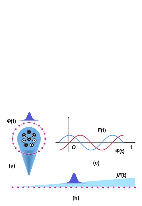
Figure 1: (Color online) The schematic illustrations for a tight-binding ring threaded by a time-dependent magnetic flux $\Phi\left(t\right)$ in (a) from (1), and a chain subjected to a time-dependent external field $F\left(t\right)$ in (b) from (13), where $j$ denotes the lattice site. The flux and the external field is illustrated in (c), which are, but not necessary, time-periodic.

2.1 Finite ring

Consider a ring lattice with $N$ sites threaded by a magnetic field, as illustrated schematically in Figure 1(a). The Hamiltonian of the corresponding tight-binding model

$$H_{\mathrm{B}}=-J\sum_{j=1}^{N}\left(\rme^{\rmi 2\pi\Phi\left(t\right)/N}a_{j}^{\dagger}a_{j+1}+\mathrm{H.c.}\right)$$ (1)

depends on the magnetic flux through the ring in units of the magnetic flux quantum $\Phi_{0}=h/e$. Here $a_{j}^{\dagger}$ is the creation operator of a particle at the $j$th site with periodic boundary conditions. The flux does not exert force on the Bloch electrons but can change the local phase of its wave function due to the Aharonov-Bohm (AB) effect. Note that the particle is not restricted to be either bosons or fermions.

By the transformation

$$a_{j}=\frac{1}{\sqrt{N}}\sum_{k}\rme^{\rmi kj}a_{k},$$ (2)

where $k=2\pi n/N$ and $n\in\left[1,N\right]$, the Hamiltonian can readily be written as

$$H_{\mathrm{B}}=-2J\sum_{k}\cos\left(k+\phi\left(t\right)\right)a_{k}^{\dagger}a_{k},$$ (3)

with $\phi\left(t\right)=2\pi\Phi\left(t\right)/N$, and the corresponding eigenstate takes the form of

$$\left|k\right\rangle=\frac{1}{\sqrt{N}}\sum_{j}\rme^{\rmi kj}\left|j\right\rangle.$$ (4)

Note that the time-dependent Hamiltonian possesses fixed instantaneous eigenstates, while the flux solely affects the instantaneous eigenvalues. This will be crucial for employing such a setup to investigate the control of a quantum state since the exact solutions of a time-dependent Hamiltonian are rare.

The evolution of an arbitrary state under the Hamiltonian $H$ is dictated by the unitary operator

$$U\left(t^{\prime},t\right)=\mathcal{T}\exp\left(-i\int_{t}^{t^{\prime}}H\left(t^{\prime\prime}\right)\rmd t^{\prime\prime}\right),$$ (5)

where $\mathcal{T}$ denotes the time-ordering operator, which yields the propagator represented in the momentum and the spatial eigenstates

$$U_{k^{\prime}k}\left(t^{\prime},t\right)= \left\langle k^{\prime}\right|U\left(t^{\prime},t\right)\left|k\right\rangle =\exp\left[\rmi 2Jf_{k}\left(t^{\prime},t\right)\right]\delta_{k^{\prime}k},$$ (6)

$$U_{j^{\prime}j}\left(t^{\prime},t\right)= \left\langle j^{\prime}\right|U\left(t^{\prime},t\right)\left|j\right\rangle =\frac{1}{N}\sum_{k}\exp\left[\rmi 2Jf_{k}\left(t^{\prime},t\right)\right]\rme^{\rmi k\left(j^{\prime}-j\right)},$$ (7)

where

$$f_{k}\left(t^{\prime},t\right) = \int_{t}^{t^{\prime}}\cos\left[k+\phi\left(t^{\prime\prime}\right)\right]\rmd t^{\prime\prime}=\cos\left(k\right)u+\sin\left(k\right)v$$ (8)

$$= \sqrt{u^{2}+v^{2}}\cos\left[k+\varphi\left(t^{\prime},t\right)\right].$$

Here the time-dependent functions are defined as

$$\varphi\left(t^{\prime},t\right) = \arg\left(u-iv\right),$$ (9)

$$\qquad u = \int_{t}^{t^{\prime}}\cos\left[\phi\left(t^{\prime\prime}\right)\right]\rmd t^{\prime\prime},$$ (10)

$$\qquad v = \int_{t}^{t^{\prime}}\sin\left[\phi\left(t^{\prime\prime}\right)\right]\rmd t^{\prime\prime}.$$ (11)

Thus, the propagator can be obtained in the following explicit form

$$U_{k^{\prime}k}\left(t^{\prime},t\right)=\exp\left(\rmi 2J_{\mathrm{eff}}\cos\left[k+\varphi\left(t^{\prime},t\right)\right]\left(t^{\prime}-t\right)\right)\delta\left(k^{\prime}-k\right)$$ (12)

with

$$J_{\mathrm{eff}}=J\sqrt{u^{2}+v^{2}}/\left(t^{\prime}-t\right).$$

Its physical interpretation is very clear: the time evolution of the state at instant $t^{\prime}$ is equivalent to that governed by a uniform ring with hopping strength $J_{\mathrm{eff}}$ threaded by the flux $N\varphi\left(t^{\prime},t\right)$. We note that such an equivalence is always true for an arbitrary time-dependent function of the flux $\phi\left(t\right)$. In the following, we will discuss its application together with the propagator of the infinite chain system.

2.2 Infinite chain

Now we turn to an infinite chain system driven by a time-dependent homogeneous field, as illustrated schematically in Figure 1(b). The Hamiltonian of the corresponding tight-binding model is

$$H_{\mathrm{E}}=-J\sum_{j=-\infty}^{\infty}\left(a_{j}^{\dagger}a_{j+1}+\mathrm{H.c.}\right)+F\left(t\right)\sum_{j=-\infty}^{\infty}jn_{j}.$$ (13)

In the case of a constant external field $F_{0}$, the dynamics of a localized wave packet exhibit coherent oscillations with period $\tau_{\mathrm{BO}}=2\pi/F_{0}$, i.e. Bloch oscillations, instead of the expected accelerated motion towards infinity [10]. This non-intuitive feature arises from the discreteness of the system.

Over the past several decades, such a system has been investigated extensively for potential applications. Most of them focus on the static or time-periodic fields. In this study, we investigate the case of arbitrary time-dependent homogeneous fields.

Unlike the system of (1) discussed above, the instantaneous eigenfunctions are no longer independent of time. However, they can be obtained explicitly on the basis of the Stark ladder theory [11]. For the time-dependent Hamiltonian, according to the framework of Feynman’s polygonal path approach, the propagator can be presented as a functional integration

$$U_{k^{\prime}k}\left(t^{\prime},t\right)=\int_{k}^{k^{\prime}}\exp\left(-\rmi\int_{t}^{t^{\prime}}H\left(k^{\prime\prime},t^{\prime\prime}\right)\rmd t^{\prime\prime}\right)\mathcal{D}\left(k^{\prime\prime}\right),$$ (14)

where the integration denotes the time evolution through different paths from $k$ to $k^{\prime}$ in the momentum space [12].

For an infinitesimal time interval $\rmd t$, the propagator can be obtained from that of the time-independent Hamiltonian, which has the form

$$U_{k^{\prime}k}\left(t+\rmd t,t\right)=\exp\left(-\rmi 2J\frac{\sin\left(k^{\prime}\right)-\sin\left(k\right)}{F\left(t\right)}\right)\delta\left(k^{\prime}-k+F\left(t\right)\rmd t\right).$$ (15)

Considering a finite time interval $t^{\prime}-t$, where $t$ and $t^{\prime}$ denote the initial and final, respectively, the propagator can be expressed in the form

$$U_{k^{\prime}k}\left(t^{\prime},t\right)=\exp\left(\rmi 2J_{\mathrm{eff}}\cos\left[k+\varphi\left(t^{\prime},t\right)\right]\left(t^{\prime}-t\right)\right)\delta\left(k^{\prime}-k+I\left(t^{\prime},t\right)\right).$$ (16)

Here

$$J_{\mathrm{eff}}=J\sqrt{u^{2}+v^{2}}/\left(t^{\prime}-t\right)$$ (17)

acts as the time-dependent effective hopping amplitude of a uniform chain, and

$$I\left(t^{\prime},t\right)=\int_{t}^{t^{\prime}}F\left(t^{\prime\prime}\right)\rmd t^{\prime\prime}$$ (18)

denotes the impulse of force during the time interval $t^{\prime}-t$, and

$$\varphi\left(t^{\prime},t\right)=\arg\left(u-\rmi v\right)$$ (19)

is the phase shift, where

$$u = \int_{t}^{t^{\prime}}\cos\left[I\left(t^{\prime\prime},t\right)\right]\rmd t^{\prime\prime},$$ (20)

$$v = \int_{t}^{t^{\prime}}\sin\left[I\left(t^{\prime\prime},t\right)\right]\rmd t^{\prime\prime}.$$ (21)

One can see that the propagators of the two systems $H_{\mathrm{B}}$ and $H_{\mathrm{E}}$ have similar form, while there are still several differences between them: First, the allowed momentum values are different. The former is discrete for the finite site ring, whereas the latter must be continuous. Second, in a ring system, the momentum is always conservative according to the factor $\delta_{k^{\prime}k}$ in (12), whereas it is not in the chain system, suggesting that one can extend the Bloch’s acceleration theorem to the momentum-impulse theorem as

$$k^{\prime}=k-I\left(t^{\prime},t\right)$$ (22)

for an arbitrary $F\left(t\right)$, which is the central result of this study. Despite the difference between the two systems, we discuss in the next section that they are equivalent for dealing with the dynamics of a wide wave packet if we take $F\left(t\right)=-\partial\phi\left(t\right)/\partial t$.

3 Wave packet dynamics

In this section, we will apply the propagator to a specific case: the time evolution of a GWP in a system driven by an arbitrary time-dependent external field. We will briefly rederive the basic results for the system of cosinoidal fields based on the exact evolved wave function, which offers various advantages over the traditional approach. In the following, we restrict the discussion to the GWP on the lattice, with

$$\left|\psi\left(0\right)\right\rangle=\left|\Psi\left(k_{0},N_{\mathrm{A}}\right)\right\rangle=\Lambda\sum_{k}\exp\left[-\frac{\left(k-k_{0}\right)^{2}}{\alpha^{2}}-\rmi N_{\mathrm{A}}k\right]\left|k\right\rangle,$$ (23)

where $\Lambda$ is the normalization factor, where $k_{0}$ and $N_{\mathrm{A}}$ denote the central momentum and position of the initial wave packet, respectively.

Applying the propagator in (16), we obtain the evolved wave function at time $t$ as

$$\left|\psi\left(t\right)\right\rangle = \sum_{k}U_{kk^{\prime}}\left(t,0\right)\left\langle k^{\prime}\right.\left|\psi\left(0\right)\right\rangle\left|k\right\rangle$$ (24)

$$= \Lambda\rme^{-\rmi N_{\mathrm{A}}I\left(t\right)}\sum_{k}\exp\left(-\frac{\left(k+I\left(t\right)-k_{0}\right)^{2}}{\alpha^{2}}\right)$$

$$\times\exp\left(\rmi 2J_{\mathrm{eff}}\left(t\right)\cos\left[k+I\left(t\right)+\phi\left(t\right)\right]t-\rmi N_{\mathrm{A}}k\right)\left|k\right\rangle.$$

In the case of a wide wave packet, i.e. $\alpha\ll 1$, it can be reduced as

$$\left|\psi\left(t\right)\right\rangle\approx\exp\left(\rmi\gamma\left(t\right)\right)\left|\Psi\left(k_{0}-I\left(t\right),N_{\mathrm{A}}+D\left(t\right)\right)\right\rangle,$$ (25)

where

$$\gamma\left(t\right)=2J_{\mathrm{eff}}\left(t\right)\cos\left(k_{0}+\varphi\left(t\right)\right)t-N_{\mathrm{A}}I\left(t\right)$$ (26)

is an overall phase factor, and thus can be neglected when only a single wave packet is considered. Here

$$D\left(t\right)=2J_{\mathrm{eff}}\left(t\right)\sin\left[k_{0}+\varphi\left(t\right)\right]t$$ (27)

denotes the displacement of the centre of the wave packet. It is interesting to find that the evolved state $\left|\psi\left(t\right)\right\rangle$ is still a GWP with the same shape as the initial one. The shape is retained because of the field homogeneity and the wide GWP approximation. Nevertheless, even for a narrow wave packet, the periodicity of the propagator ensures the revival of shape. In any case, the displacement $D\left(t\right)$ is crucial for characterizing the dynamics of the wave packet. However, it may have a complex dependence on the parameters of the driving force. Fortunately, when we deal with the group velocity $v_{\mathrm{g}}\left(t\right)=\partial D\left(t\right)/\partial t$, the physical picture will become clear. Actually, the straightforward algebra shows that

$$v_{\mathrm{g}}\left(t\right)=2J\sin\left[k_{0}-I\left(t\right)\right],$$ (28)

which accords with the fact that the central momentum of the wave packet $k_{0}-I\left(t\right)$ originates from the momentum-impulse theorem in the former section. We notice that the instantaneous group velocity is solely determined by the impulse $I\left(t\right)$, but not the details of the field function $F\left(t\right)$. In the following, we apply this conclusion to some special cases to demonstrate its validity and its application in QIP.

On the other hand, we can investigate the relationship of the two models in (1) and (13) through the dynamics of the wave packet. By performing the same procedure as above, we can obtain the evolved GWP under the system of (1) as

$$\left|\psi\left(t\right)\right\rangle\approx\rme^{\rmi\gamma\left(t\right)}\left|\Psi\left(k_{0},N_{\mathrm{A}}+D\left(t\right)\right)\right\rangle$$ (29)

if the the width of the wave packet is far smaller than the length of the ring. Here

$$\gamma\left(t\right)=2J_{\mathrm{eff}}\left(t\right)\left[\cos\left(k_{0}+\varphi\left(t\right)\right)+\sin\left(k_{0}+\varphi\left(t\right)\right)k_{0}\right]t,$$ (30)

and

$$D\left(t\right)=2J_{\mathrm{eff}}\left(t\right)\sin\left[k_{0}+\varphi\left(t\right)\right]t.$$ (31)

Note that the evolved state of (25) differs from that of (25) in that there is no momentum shift of the wave packet in the flux-pierced ring. Nevertheless, its group velocity is expressed as

$$v_{\mathrm{g}}\left(t\right)=2J\sin\left[k_{0}+\phi\left(t\right)\right],$$ (32)

which has the same form as that in (28). A comparison of (25) and (29) clearly shows that by taking the substitution of

$$\phi\left(t\right)=-I\left(t\right),$$ (33)

i.e. $F\left(t\right)=-\partial\phi\left(t\right)/\partial t$, the probability distributions of the two evolved wave packets are identical. Therefore, when the probability current is measured, the two systems are equivalent within a local range. It accords with Faraday’s law of induction in classical physics, wherein a changing magnetic flux induces an electric field. In the following, we focus the discussions on the chain system, because the results can be simply extended to those of the ring system.

It is worth mentioning that the group velocity $v_{\mathrm{g}}$ of (32) can be understood in the following simple manner: as is well known, the group velocity in real space is determined by the dispersion relation with respect to $k$. For the system $H_{\mathrm{B}}$ of (1), the derivative of the instantaneous dispersion relation in (3), $\varepsilon_{k}=-2J\cos\left[k+\phi\left(t\right)\right]$ can directly obtain the group velocity expressed in (32). For the system $H_{\mathrm{E}}$ of (13), we can also obtain the group velocity from the derivative of the basal dispersion relation, which originates from the spectrum of a uniform tight-binding chain of $\varepsilon_{k}=-2J\cos\left(k\right)$. Meanwhile, because of electric field effect, the momentum shifts.The central momentum of the evolved GWP is presented by $k_{0}\left(t\right)=k_{0}-I\left(t\right)$, which yields the group velocity of (28).

3.1 Bloch oscillations

Now, we consider the simplest case of an external static field $F\left(t\right)=F_{0}>0$ subjected to an infinite chain system (or equivalently, with a pierced flux $\phi\left(t\right)=-F_{0}t$ in a finite ring system). It is well known that Bloch oscillations occur in this system. This phenomenon can be revisited in the framework of the propagator, which is introduced as above. Moreover, the results can be extended to the case of a finite ring. It is also a starting place for the discussion of more complicated cases in the next sections.

In this case, we have

$$I\left(t\right)=F_{0}t.$$ (34)

Because of the discreteness of the lattice, the momentum space is restricted in the first Brillouin zone. Also, the Bragg reflections give the Bloch oscillations directly. From the former analysis, we can get

$$D\left(t\right) = \frac{2J}{F_{0}}\left[\cos\left(k_{0}-F_{0}t\right)-\cos\left(k_{0}\right)\right],$$ (35)

$$v_{\mathrm{g}}\left(t\right) = 2J\sin\left(k_{0}-F_{0}t\right),$$ (36)

with the period

$$\tau_{\mathrm{BO}}=\frac{2\pi}{F_{0}}$$ (37)

and the extent of the Bloch oscillations

$$L_{\mathrm{BO}}=\frac{4J}{F_{0}}.$$ (38)

3.2 Bloch translation

In the following, we will revisit the dynamics of a wave packet subjected to a periodic time-modulated field $F(t)$ with the aid of the propagator, which offers advantages over the traditional approach. First, let us consider the external field in the form

$$F\left(t\right)=n\omega+F_{\mathrm{A}}\cos\left(\omega t\right),$$ (39)

where $n$ is an integer representing the DC field, and $F_{\mathrm{A}}$ is a constant representing the AC field. According to our former analysis, we have

$$I\left(t\right)=n\omega t+\frac{F_{\mathrm{A}}}{\omega}\sin\left(\omega t\right),$$ (40)

and

$$v_{\mathrm{g}}\left(t\right)=2J\sin\left[k_{0}-n\omega t-\frac{F_{\mathrm{A}}}{\omega}\sin\left(\omega t\right)\right].$$ (41)

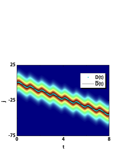
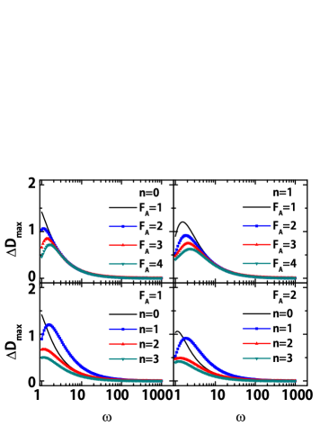
Figure 2: (Color online) The time evolutions of a Gaussian wave packet (GWP) are plotted of the envelopes with time $t$ (left) and the shaking deviations with the field frequency $\omega$ (right). The envelopes are calculated by exact diagonalization from (15), where the external field is $n=1$, $F_{\mathrm{A}}=1$ and $\omega=1$. The displacement (27) and the average displacement (43) are marked by the solid circle and line in units of the lattice site, where $t$ is in units of $\tau=2\pi/\omega$. The maximum shaking amplitudes $\Delta D_{\mathrm{max}}$ from (44) of the same wave packet are plotted under the fields with different $n$, $F_{\mathrm{A}}$ (in units of $J$) and $\omega$ (in units of $J$). The wave packet from (23) has $\alpha=0.1$ and central momentum $k_{0}=\pi/2$ on an $N=200$ chain with hopping amplitude $J=1$. It shows that the GWP moves straightly with small shaking, which is depressed under high frequency external field.

We notice that $v_{\mathrm{g}}\left(t\right)$ is a periodic function with the period $\tau=2\pi/\omega$, but the displacement in each period

$$D\left(\tau\right) = \int_{0}^{\tau}v_{\mathrm{g}}\left(t\right)\rmd t$$ (42)

$$= 2J\left(-1\right)^{n}\mathcal{J}_{n}\left(\frac{F_{\mathrm{A}}}{\omega}\right)\sin\left(k_{0}\right)\tau$$

is non-zero in general, since $v_{\mathrm{g}}\left(t\right)$ of (41) is not a monochromatic function of time $t$. Here $\mathcal{J}_{n}\left(z\right)$ denotes the Bessel function of the first kind. Then, the wave packet exhibits unidirectional motion with a periodic shaking, which can be referred to as the Bloch translation.

Considering a long time scale of $t\gg\tau$, we have

$$\overline{D}\left(t\right)\approx 2J\left(-1\right)^{n}\mathcal{J}_{n}\left(\frac{F_{\mathrm{A}}}{\omega}\right)\sin\left(k_{0}\right)t,$$ (43)

which indicates the aperiodicity of the displacement. The wave packet evolves as if in a uniform tight-binding chain, with the effective hopping amplitude $J_{\mathrm{eff}}=J\left|\mathcal{J}_{n}\left(F_{\mathrm{A}}/\omega\right)\right|$. Meanwhile, the deviation of the central position from its average

$$\Delta D=D\left(t\right)-\overline{D}\left(t\right)$$ (44)

is also a periodic function

$$\Delta D\left(t+\tau\right)=\Delta D\left(t\right).$$ (45)

Then, the wave packet moves in one direction accompanied by small shaking. From (41), the instantaneous velocity $v_{\mathrm{g}}\left(t\right)$ is a bounded function with $\left|v_{\mathrm{g}}\left(t\right)\right|\leq 2J$. And we have

$$\lim_{\omega\rightarrow\infty}\Delta D\left(t\right)=0,$$ (46)

because the period $\tau$ goes to infinitesimal. This indicates that the shaking disappears as the frequency increases, which is shown in Figure 2. Then, the wave packet moves uniformly with a constant velocity $2J_{\mathrm{eff}}\sin\left(k_{0}\right)$.

In principle, the wave packet can be coherently stopped when an appropriate $F_{\mathrm{A}}$ is taken to make $\mathcal{J}_{n}\left(F_{\mathrm{A}}/\omega\right)=0$. We will consider this problem for the two cases $n=0$ and $n\geq 1$. For the zeroth-order Bessel function of the first kind, we have $\mathcal{J}_{0}\left(F_{\mathrm{A}}/\omega\right)=0$ when $F_{\mathrm{A}}/\omega=0.768\pi$, etc., which are the roots of the Bessel function. It indicates that one should take frequency-dependent $F_{\mathrm{A}}$ to obtain DD. As for the ring system with the magnetic flux as a monochromatic wave of

$$\phi\left(t\right)=\phi_{\mathrm{A}}\sin\left(\omega t\right),$$ (47)

it corresponds to $\phi_{\mathrm{A}}=-F_{\mathrm{A}}/\omega=-0.768\pi$, which accords with the results in our previous study [7]. Nevertheless, in the case of $n\geq 1$, it becomes simple since the property of the Bessel function makes $\mathcal{J}_{n}\left(0\right)=0$ for $n\geq 1$. Thus, in such a case, DD can be realized for any finite value of $F_{\mathrm{A}}$ in the limit of $\omega\rightarrow\infty$.

3.3 Super Bloch oscillations

Now, we consider the external field in the form of

$$F\left(t\right)=\left(n+\delta\right)\omega+F_{\mathrm{A}}\cos\left(\omega t\right),$$ (48)

where $n$ is an integer, and $\delta$ is the detuning factor. Such a model has been studied extensively by the equation of motion for the average of the observables. In this study, we revisit it by investigating the time evolution of the wave function. Our former analysis gives

$$I\left(t\right)=n\omega t+\delta\omega t+\frac{F_{\mathrm{A}}}{\omega}\cos\left(\omega t\right),$$ (49)

and

$$v_{\mathrm{g}}\left(t\right)=2J\sin\left[k_{0}-n\omega t-\delta\omega t-\frac{F_{\mathrm{A}}}{\omega}\sin\left(\omega t\right)\right].$$ (50)

In this case, $v_{\mathrm{g}}\left(t\right)$ is no longer a periodic function of time $t$ with the period $\tau$. Because of the slight detuning of $\delta\ll 1$, it can be presumed that the group velocity $v_{\mathrm{g}}\left(t\right)$ still oscillates with a quasi-period $\tau$. However, the displacement during each quasi-period is not invariable and can change its sign at a certain instant. More precisely, the one-period displacement is given by (43) as

$$D\left(\tau\right)\approx 2J\left(-1\right)^{n}\mathcal{J}_{n}\left(\frac{F_{\mathrm{A}}}{\omega}\right)\sin\left(k_{0}-\delta\omega t\right)\tau,$$ (51)

which is a periodic function with a long period

$$\tau_{\mathrm{SBO}}=\frac{2\pi}{\delta\omega}$$ (52)

approximately. Accordingly, the one-period average displacement has the form

$$\overline{D}\left(t\right) = \sum_{l=1}^{\mathrm{Int}\left(t/\tau\right)}\int_{\left(l-1\right)\tau}^{l\tau}v_{\mathrm{g}}\left(t^{\prime}\right)\rmd t^{\prime}$$ (53)

$$\approx 2J\frac{\left(-1\right)^{n}}{\delta\omega}\mathcal{J}_{n}\left(\frac{F_{\mathrm{A}}}{\omega}\right)\left[\cos\left(k_{0}-\delta\omega t\right)-\cos\left(k_{0}\right)\right],$$

where $\mathrm{Int}$ denotes the greatest integer function.

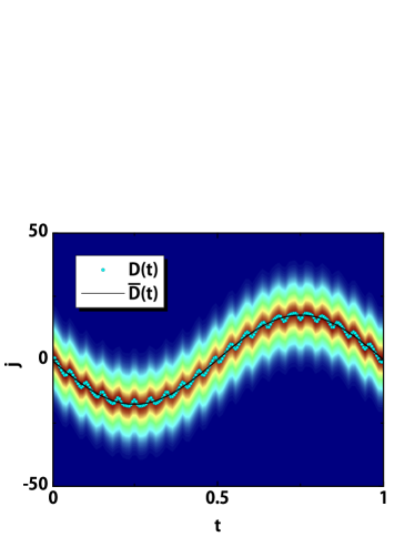
Figure 3: (Color online) The envelope of the same GWP on the same chain as shown in the left of Figure 2, while with a detuning $\delta=0.02$ of the external field and $t$ in units of $\tau_{\mathrm{SBO}}$ from (52). It shows that the GWP behaves super Bloch oscillations with large extent and small shaking.

We can see that $\overline{D}\left(t\right)$ has the same form of the customary Bloch oscillations as (35) in an infinite chain system with the following effective hopping amplitude and the static force of

$$J_{\mathrm{eff}} = J\left|\mathcal{J}_{n}\left(\frac{F_{\mathrm{A}}}{\omega}\right)\right|,$$ (54)

$$F_{\mathrm{eff}} = \delta\omega.$$ (55)

This has been termed super Bloch oscillations with the extent

$$L_{\mathrm{SBO}}=\frac{4J_{\mathrm{eff}}}{F_{\mathrm{eff}}}=4J\left|\frac{\mathcal{J}_{n}\left(\frac{F_{\mathrm{A}}}{\omega}\right)}{\delta\omega}\right|.$$ (56)

We can get the average group velocity as

$$\overline{v}_{\mathrm{g}}\left(t\right) = \frac{\partial\overline{D}\left(t\right)}{\partial t}$$ (57)

$$= -2J\left(-1\right)^{n}\mathcal{J}_{n}\left(\frac{F_{\mathrm{A}}}{\omega}\right)\sin\left(k_{0}-\delta\omega t\right).$$

Obviously, $\overline{v}_{\mathrm{g}}\left(t\right)$ is periodic with the period $2\pi/\delta\omega$, which is the period of the super Bloch oscillations. To illustrate our analysis, Figure 3 shows plots of $D\left(t\right)$ in (27) and $\overline{D}\left(t\right)$ in (53) as the functions of time $t$ in units of $\tau_{\mathrm{SBO}}$. For comparison, we also plot the profile of the time evolution of a wave packet, which is directly computed from (15) by the exact diagonalization of the finite-size Hamiltonians $H\left(n\epsilon\right)$ with $\epsilon=0.01/J$. This shows that our analysis is in agreement with the numerical simulation and provides a more exact picture of super Bloch oscillations.

4 Quantum state manipulation

Coherent quantum state storage and transfer via a coupled qubit system are crucial in the emerging area of QIP. The essence of such a process is the time evolution of a local wave packet in a discrete system. In the design of the scheme for quantum state transfer, two types of external control are usually employed: one adiabatic and the other requiring sudden changes of parameters. In the first scheme, the external field is turned on and off in an adiabatic manner. Then, the quantum state is fixed on the superposition of the instantaneous eigenstates. This requires a sufficiently long relaxation time to satisfy the adiabatic approximation condition. Therefore, decoherence becomes incredibly challenging for this scheme to be realized. The second scheme requires a stepwise change of the external field, which is difficult to accomplish practically. The scheme that employs the diabatic process shows more promise. The main difficulty with accomplishing this task in a quantum network is the tricky issue in quantum mechanics, which is the time evolution of a time-dependent Hamiltonian.

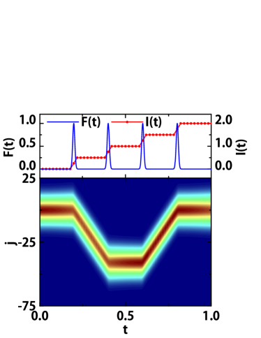
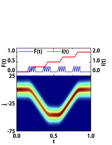
Figure 4: (Color online) The envelopes of the time evolution of same Gaussian wave packet (GWP) on the same chain as that in Figure 2, with different trains of pulsed field $F\left(t\right)$ which are Gaussian (left) and sawtooth-like (right), where $j$ is in units of the lattice site, $F\left(t\right)$ is in units of $J$, the impulse of the train accumulation $I\left(t\right)$ is in units of $\pi$, and $t$ is in units of $N/2J$. We can see that the group velocity is changed at the end of each pulse. The dynamics under the two trains has the same behaviour despite the details during the changes.

According to our former analysis, the analytical evolved wave function in the present two systems can be obtained for an arbitrary time-dependent external field. Furthermore, it reveals an interesting feature of the wave packet dynamics: the wave packet preserves its shape for an arbitrary profile of the time-modulated external field $F(t)$ owing to the homogeneity of force in space, while the momentum of the wave packet changes according to the impulse-momentum theorem. This enables us to propose such a scheme, in which the adiabaticity of the tuning process is not required. We illustrate this point as follows.

We consider the linear potential as being a Gaussian-pulse train, which can be expressed as

$$F\left(t\right) = \sum_{n}F_{n}\left(t\right),$$ (58)

$$F_{n}\left(t\right) = \frac{\sqrt{\pi}}{2\sigma}\exp\left[-\frac{\left(t-T_{n}\right)^{2}}{\sigma^{2}}\right],$$ (59)

where $\sigma$ determines the duration of each pulse. In the case $T_{n+1}-T_{n}\gg\sigma$, we have the impulse as

$$I_{n}=\frac{\sqrt{\pi}}{2\sigma}\int_{-\infty}^{\infty}F_{n}\left(t\right)\rmd t=\frac{\pi}{2}.$$ (60)

Here we choose the impulse to be $\pi/2$ since it is the minimal momentum difference between the static and the fastest-moving wave packets. According to the above results, a GWP acquires an extra momentum $\pi/2$ after each pulsed field. For an initial GWP with $k_{0}=0$, $I_{1}$ should accelerate it to the momentum of $\pi/2$ with the speed of $2J$, and $I_{2}$ should shift its momentum to $\pi$, i.e. stops it. The next field pulse $I_{3}$ turns it back and the final pulse $I_{4}$ stops it. This behaviour is illustrated in Figure 4, which shows the time evolution for an initially motionless GWP in a field composed by a sequence of four identical pulses with $\sigma=0.886$ and $t_{n}=nN/10J$, $n=1,2,3$ and $4$. The time evolution is directly computed from (15) by exact diagonalization of the finite-sized Hamiltonians $H\left(n\epsilon\right)$ with $n=\left[0,1.7\times 10^{4}\right]$ and $\epsilon=5.9\times 10^{-3}/J$. The speed of the wave packet is changed at the end of each pulse. This behaviour illustrates the expected phenomena of accelerating, stopping and turning of the wave packet.

Furthermore, if the external pulsed field is not Gaussian-like, but arbitrarily shaped with the same impulse (the area of the pulse), the result should be the same. To demonstrate this, we compute the time evolution for a sawtooth-pulsed train in Figure 4. We can see that despite the turning points, the different pulse train gives the same result in controlling the wave packet, and because of the accumulation of impulse, the amplitude of the external field can be lowered by extending the width of the pulses in the train. When being applied along with the control scheme, this coherent accelerating stopping turning scheme provides a useful strategy for the efficient coherent transfer of a quantum state.

5 Summary

In conclusion, the exact propagators of these two one-dimensional systems have shown that the Bloch acceleration theorem can be generalized to the impulse-momentum theorem in a quantum version, which connects the impulse not only to the shift of the momentum but also to the phase change of the matter waves. It has been theoretically shown that accelerating, stopping coherently and transferring a wave packet to a location on demand can be realized by exploiting the time-dependent external field. The proposed scheme is less distinct than the adiabatic process and provides a noteworthy example of coherent quantum control with high fault tolerance. It offers an advantage in that neither the precise modulation of field pulses nor adiabatic conditions for the dynamical field changes are necessarily required.

References

References

- [1] M S Byrd, L A Wu and D A Lidar 2004 J. Mod. Opt. 51 2449
- [2] C Search and P R Berman 2000 Phys. Rev. Lett.85 2272
- [3] L Zhou, S Yang, Y X Liu, C P Sun and F Nori 2009 Phys. Rev.A 80 062109
- [4] A Eckardt, C Weiss and M Holthaus 2005 Phys. Rev. Lett.95 260404 A Eckardt and M Holthaus 2007 Europhys. Lett. 80 50004
- [5] H Lignier, C Sias, D Ciampini, Y Singh, A Zenesini, O Morsch and E Arimondo 2007 Phys. Rev. Lett.99 220403
- [6] S Yang, Z Song and C P Sun 2006 Phys. Rev.A 73 022317
- [7] W H Hu and Z Song 2011 Phys. Rev.A 84 052310
- [8] André Eckardt, Christoph Weiss and Martin Holthaus 2005 Phys. Rev. Lett.95 260404
- [9] K Kudo and T S Monteiro 2010 Phys. Rev.A 83 053627
- [10] H Fukuyama, R A Bari and H C Fogedby 1973 Phys. Rev.B 8 5579
- [11] T Hartmann, F Keck, H J Korsch and S Mossmann 2004 New J. Phys.6 2
- [12] A Balaž, I Vidanović, A Bogojević, A Belić and A Pelster 2011 J. Stat. Mech. P03004 A Balaž, I Vidanović, A Bogojević, A Belić and A Pelster 2011 J. Stat. Mech. P03005