The evolution of interdisciplinarity in physics research

Abstract

Science, being a social enterprise, is subject to fragmentation into groups that focus on specialized areas or topics. Often new advances occur through cross-fertilization of ideas between sub-fields that otherwise have little overlap as they study dissimilar phenomena using different techniques. Thus to explore the nature and dynamics of scientific progress one needs to consider the large-scale organization and interactions between different subject areas. Here, we study the relationships between the sub-fields of Physics using the Physics and Astronomy Classification Scheme (PACS) codes employed for self-categorization of articles published over the past 25 years (1985-2009). We observe a clear trend towards increasing interactions between the different sub-fields. The network of sub-fields also exhibits core-periphery organization, the nucleus being dominated by Condensed Matter and General Physics. However, over time Interdisciplinary Physics is steadily increasing its share in the network core, reflecting a shift in the overall trend of Physics research.

Introduction

Scientific progress has been seen both as a succession of incremental refinements as well as a succession of epochs with relatively slow or little change that are punctuated by periods of revolutionary transitions. In Popper’s view popper , science proceeds by gradually falsifying competing candidate theories, whereas Kuhn Kuhn62 argues that during episodes of “normal science”, scientists gradually improve their theories within the current framework until enough unexplainable anomalies emerge to call for a major paradigm shift. Such shifts have occurred on many scales, from scientific revolutions with global reverberations to smaller breakthroughs within specific fields or sub-fields of science. However, this view ignores the possibility of entirely new avenues of research emerging from new connections that are forged between apparently disjoint areas of science. Thus, new paradigms may be born not only because of evidence that contradicts existing theories, but also because entirely new questions and theoretical frameworks appear. For example, consider the rise of systems biology, driven by technological advances in data acquisition and their analysis through computer algorithms, or the emergence of network science that merges aspects from physics, computer science, and social sciences.

In this paper, we focus on the dynamics and emergence of connections between the various subfields of physics, and perform a longitudinal analysis of the evolution of physics from 1985 till 2009. Our results are based on a study of the papers appearing in the Physical Review series of journals (Physical Reviews A, B, C, D, E, Physical Review Letters and Review of Modern Physics) published by the American Physical Society during this period, with their Physics and Astronomy Classification Scheme (PACS) numbers indicating the subfields of physics to which they belong. If a paper is listed under two different PACS codes, the two corresponding sub-fields are considered to be connected by the paper. In this manner we construct a set of annual snapshots of the networks of sub-fields in physics that are connected through all papers that have been published in each year, and study the evolution of these networks at multiple structural scales. In this way, we can focus on the big picture of the evolution of physics in terms of changes in the nature of connections between its subfields, instead of the microscopic level that is considered by the widely studied collaboration or citation networks Newman01a ; Redner98 ; Pan12 ; Redner05 .

We show that the network of the subfields of physics is becoming increasingly connected over time, both in terms of link density and the numbers of papers joining different subfields. Despite gradual changes in the network density, composition, and degrees of individual nodes, all key statistical distributions display scaling, indicating stationarity in the underlying micro-dynamics Gautreau09 . It is seen that a substantial and increasing fraction of new links connects nodes that belong to dissimilar branches of the PACS hierarchy, reflecting a trend where inter-disciplinarity between the subfields of physics clearly increases. By applying the $k$-shell decomposition technique, we show that the core of physics has been dominated by Condensed Matter and General Physics for the entire period under study, with Interdisciplinary Physics steadily increasing its importance in the core. It is seen that a substantial and increasing fraction of new links connects nodes that belong to dissimilar branches of the PACS hierarchy, reflecting a trend where interdisciplinarity between the subfields of physics clearly increases. By applying the $k$-shell decomposition technique, we show that the core of physics has been dominated by Condensed Matter and General Physics for the entire period under study, with Interdisciplinary Physics steadily increasing its importance in the core.

Results

We have analyzed all published articles in Physical Review (PR) journals APS from 1985 till the end of 2009 which are classified by their authors as belonging to certain specific sub-fields using the corresponding PACS codes. The PACS is an internationally adopted, hierarchical subject classification system of the American Institute of Physics (AIP) for categorizing publications in physics and astronomy PACS . It is primarily divided into 10 top-level categories that represent broad research areas. Each of these categories are then divided into smaller domains representing more specific fields of physics, which may be further split into even more specific sub-fields. Thus, each of these PACS codes represent a specific sub-field of physics. (for a detailed description of the data, see Methods). For constructing the networks of the different sub-fields, we consider the PACS codes as nodes, a pair of which are linked if an article is classified by both these codes. In these networks, the degree $k$ of a node corresponds to its number of links, i.e. number of other PACS codes it is connected to, and its strength $s$ to the total number of articles published with the PACS code. The numbers of papers sharing two PACS codes are accounted for with the weight $w$ of their link. In order to study the time evolution of this system, we create yearly aggregated networks by considering all the articles published in a given year (see Methods).

Network-level evolution of the system

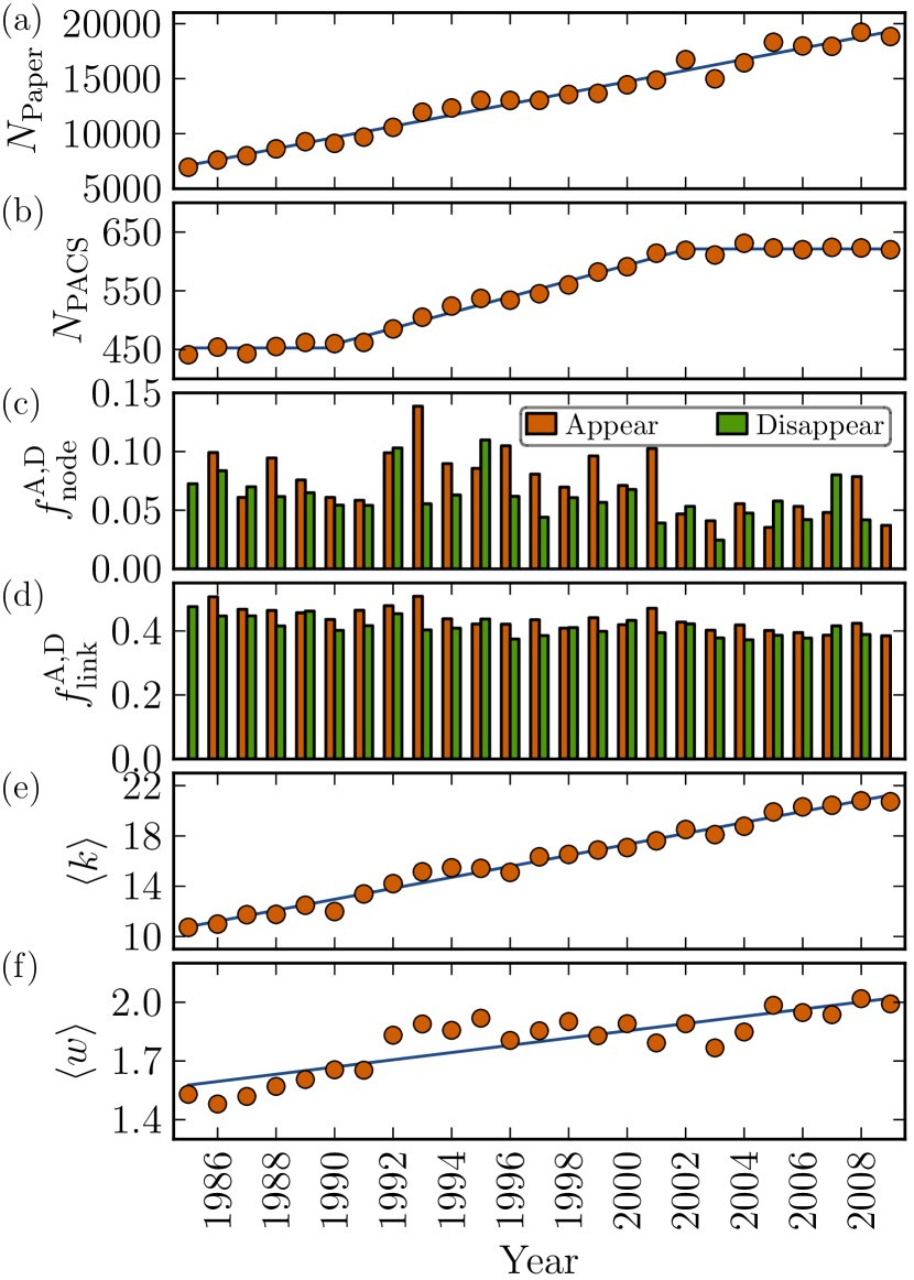
Figure 1: The time evolution of various properties of the PACS network: (a) the number of published papers, (b) the number of PACS codes, (c) the fraction of new and disappeared nodes, (d) the fraction of new and disappeared links, (e) the average degree, $\langle k\rangle$, and (f) the average link weight, $\langle w\rangle$. The solid lines in (a), (e) and (f) denote a linear growth of $\langle\Delta N_{\mathrm{Papers}}\rangle\approx 508$ papers per year, a yearly increase of $\langle\Delta k\rangle\approx 0.44$ of the average degree $\langle k\rangle$, and a yearly increase of $\langle\Delta w\rangle\approx 0.02$ of the average link weight $\langle w\rangle$, respectively. The solid line in (b) shows two roughly constant regimes, interspersed by a period of average linear increase of $\Delta N_{\mathrm{PACS}}=13.5$ PACS codes per year between 1990-2002. Note that $k$ and $w$ are heterogeneously distributed; see Fig. 2.

We begin by considering the evolution of the overall system properties between 1985 and 2009. For these 25 years, the total number of yearly publications $N_{\mathrm{Papers}}$ in all PR journals has grown linearly [Fig. 1(a)], while the number of PACS codes $N_{\mathrm{PACS}}$ shows a linear increase between 1990 and 2002, remaining roughly constant before and after this period. Note that this does not imply that the same codes have been in use in all the years prior to 1990 or those after 2002, but rather that the number of new PACS codes that were introduced each year were approximately balanced by the number of codes that were discontinued that year. The fraction of new and removed PACS codes each year is seen to fluctuate between 5% and 15% in Fig. 1(c). The yearly fractions of new and disappearing links between PACS codes are higher, fluctuating around $\sim 40\%$ [Fig. 1(d)]. When looking at network averages of the degree $\langle k\rangle$ and link weight $\langle w\rangle$ [Fig. 1(e),(f)], it is seen that not only does the number of published papers grow, but the network also becomes more connected, as both $\langle k\rangle$ and $\langle w\rangle$ grow approximately linearly. As a consequence, the average path length of the network decreases linearly (see Supplementary Information). Thus, in general, the connectivity between different subfields of physics is increasing with time.

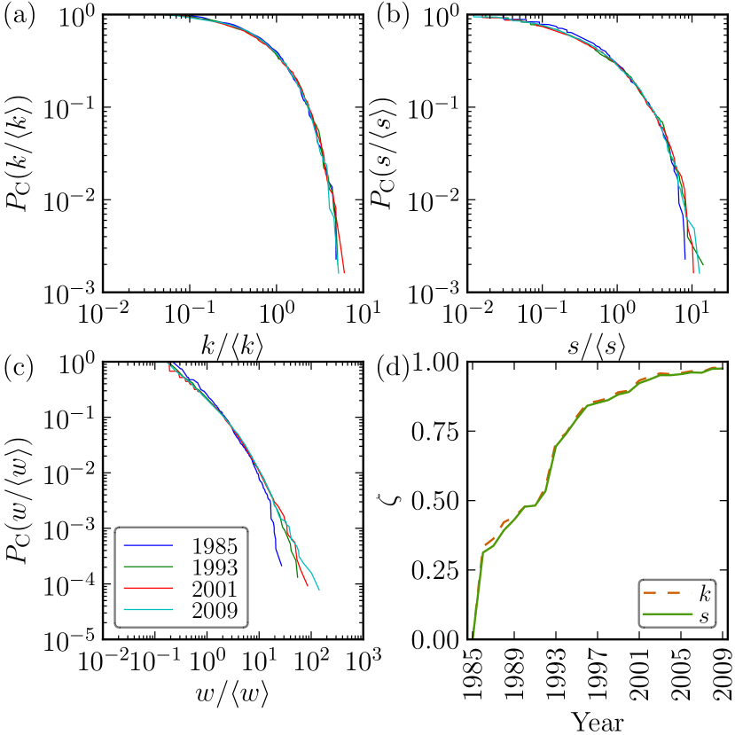
Figure 2: Stationarity of the macro-level statistical distributions and variation at the micro level with time. The cumulative distributions of (a) degree $k$, (b) strength $s$ and (c) link weight $w$ of the PACS network, for four different years. The curves have been scaled by their averages for the given year. (d) The dissimilarity coefficient $\zeta$ for the degree and strength ranks of the nodes, between the year 1985 and subsequent years.

The scaled cumulative distributions of the key quantities (degree $k$, strength $s$, and link weight $w$) are shown in Fig. 2 for four different years. All distributions are broad and indicate heterogeneity – compared to the averages, some subfields of physics are much more connected to the rest, the links between some fields are stronger, and many more papers are published in some fields. Furthermore, the overlap of the rescaled distributions indicates that although the averages of the distributions are growing over time, the functional form of the distributions remains similar Gautreau09 ; Radicchi11 . This is corroborated by comparing the Kolmogorov-Smirnov (KS) statistic of the degree distribution of the yearly networks with each other and finding that the KS distance stay at a low constant value Massey51 . A similar comparisons of the KS statistics of the strength distribution of the yearly networks show similar behavior, although there is a slight deviation from this general pattern for the year 1985 (see Supplementary Information for further details). Hence, although the composition of the system changes over time in terms of nodes and links appearing and disappearing (Fig. 1), the functional shape of the key distributions remain similar across the years, indicating stationarity at the level of macro dynamics.

In contrast to the relative invariance of the distributions, we observe that over a long time-scale the degrees and strengths of some nodes in the network increase or decrease in rank over time. Fig. 2(d) displays the dissimilarity coefficient $\zeta$ of the degree ranks Kossinets06 (see Methods) with respect to the year 1985 as a function of time; $\zeta\in[0,1]$ such that low values indicate invariant node ranks. It is seen that $\zeta$ increases monotonically with time, approaching $\zeta\approx 1$ towards the end. Thus, the degree ranks of the PACS codes change gradually over time and become uncorrelated towards the end of the period under study, indicating the presence of longer-term trends. Using the node strength to calculate $\zeta$ or calculating $\zeta$ between all pairs of years yields similar results (see Supplementary Information). We also compare the structural properties of the empirical PACS network with a randomized ensemble, in which PACS codes are reshuffled among papers. This is to see whether the observed properties of the network are expected to appear purely by chance as a consequence of the constraints inherent in the system. We found that in the randomized version there are many more links in the network compared to the empirical network leading to an increase in the clustering coefficient, decrease in the average link weight, and decrease in the average path length (see Supplementary Information).

Micro-level dynamics

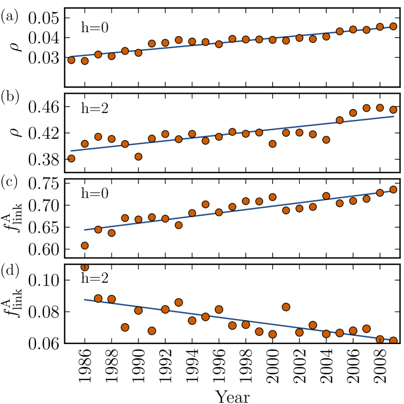
Figure 3: The time evolution of network density and newly appearing links. Evolution of the link density $\rho$ within the sets of nodes that are hierarchically (a) dissimilar, and (b) similar up to second level. Time dependence of the fraction of new links $f_{\mathrm{Links}}^{\mathrm{A}}$ that connect nodes that are hierarchically (c) dissimilar and (d) similar up to the second PACS level. The solid curves indicate linear increase in (a), (b) and (c) with slope $6.2\times 10^{-4}$, $2.2\times 10^{-3}$ and $3.9\times 10^{-3}$, respectively and linear decrease in (d) with slope $1.1\times 10^{-3}$.

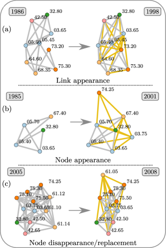
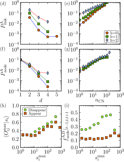
Figure 4: Micro-dynamics in the PACS network. Examples of (a) the appearance of new links that increase the density of a local neighborhood: a large number of links appear between some sub-fields of condensed matter and general physics, (b) the appearance of new nodes (03.75, 74.25) and links increasing the density and (c) changes in the network structure, where a new node (61.05) replaces several existing nodes (61.10, 61.12, 61.14). Probability of link appearance as a function of the (d) distance $d$ and (e) number of common neighbors $n_{CN}$ between the nodes. Probability of appearance of new nodes as a function of the (f) $d$ and (g) $n_{CN}$ between the nodes. The links categorized according to the hierarchical similarity $h$ of the nodes they are connecting. (h) Similarity of discontinued nodes (circles) and newly introduced nodes (squares) with their maximally similar counterpart nodes, as measured by the overlap $O_{ij}^{w}$. The overlap is averaged over focal node strength. (i) The fraction of maximally similar nodes that appear around the disappearance of the focal node (circles) (from one year before the disappearance to one year after) and the fraction of maximally similar nodes that have disappeared around the time of appearance of the focal node (squares), again as a function of focal node strength.

Next we take a detailed look at the micro-dynamics of new and disappearing links and nodes. We take advantage of the hierarchical nature of the PACS scheme (see Methods), and consider the hierarchical similarity $h$ of two PACS nodes. Nodes are considered dissimilar ($h=0$), if they belong to different main branches of the PACS hierarchy and thus represent very different subfields of physics. Nodes can also represent related subfields of physics and be similar with respect to the first level of hierarchy ($h=1$, i.e., they share their first PACS digit), or similar with respect to the second level ($h=2$, i.e., they are even more similar since they share the first two PACS digits). First, we focus on the link density $\rho$ of the network, defined for each similarity class as the number of links between nodes of the class normalized by the number of pairs of nodes in the class. The evolution of the link density between dissimilar nodes ($h=0$) and nodes belonging to the same second hierarchical level ($h=2$) is displayed in Figs. 3(a) and (b). For both cases, the density increases with time. As one would expect, the link density for $h=2$ nodes is far higher than that between dissimilar nodes. However, the relative increase of the density between the $h=0$ nodes is much higher, indicating an increasing trend where new connections emerge between the main branches of physics. If the new links of each year are split into fractions according to whether they connect similar or dissimilar sub-fields [Fig. 3(c-d)], it is seen that a substantial and increasing fraction of new links connects nodes that belong to dissimilar branches of the PACS hierarchy ($h=0$), while the fraction of new links joining similar PACS codes ($h=2$) decreases with time. Thus, there is an increase in interdisciplinarity between the subfields of physics, as dissimilar branches of the PACS hierarchy are becoming increasingly connected. This result holds even with a randomized null model that takes into account the different numbers of $h=0$ and $h=2$ nodes (see Supplementary Information). Furthermore, this hierarchical connectivity and the increase in the interdisciplinarity of the empirical network is lost in a randomized network constructed by randomly shuffling the PACS codes across different papers (see Supplementary Information).

Let us next address the role of network topology in the micro-dynamics. In particular, we want to see whether new links reflect the clustered structure of the network, increasing the density of dense neighborhoods as exemplified by the visualization of Fig. 4(a). Additionally, since the PACS numbers themselves evolve and new codes appear, local clusters may also become increasingly connected if new nodes joining nearby nodes appear, as in Fig. 4(b). The disappearance and appearance of nodes may also reflect structural changes in the PACS system, such as code replacement [Fig. 4(c)].

First, we look for evidence for the mechanisms of Fig. 4(a) and (b), where new links are not randomly created, but follow a process where dense clusters of interlinked PACS codes become even denser. For this, we determine the geodesic distance $d$ (the number of links on the shortest path) and the number of common neighbors $n_{\mathrm{CN}}$ for all pairs of nodes for each year, and count the number of pairs that are joined through a new link or through a new intermediate node in the following year. This allows us to calculate the probabilities of link and connecting node appearance ($P_{\mathrm{links}}^{\mathrm{A}}$, $P_{\mathrm{node}}^{\mathrm{A}}$) aggregated over the data interval. Their dependence on the geodesic distance and number of common neighbors is shown in Fig. 4 (d)-(g), where we have further divided all node pairs into PACS similarity classes ($h=0,1,2$ as above). It is evident that the closer the nodes are and the more common neighbors they have, the higher the likelihood of the appearance of a new direct link or a new joint neighbor connecting the nodes. The mechanisms of Figs. 4(a) and (b) are thus common in the network, and new connections between the sub-domains of physics do not emerge in a random, uncorrelated fashion; rather, connectivity increases within clusters. Furthermore, the more similar a pair of nodes is with respect to the PACS hierarchy, the higher the likelihood of new connections between them. Similar features have also been seen in other networks, e.g., in social networks new links are more likely to appear between nodes that are close, that is, nodes that have common friends or share similar interests Kossinets06 ; Granovetter73 ; Liben-Nowell05 .

In order to study code replacement dynamics of Fig. 4(c), where discontinued codes are replaced by new codes that have a similar connectivity pattern, we define a weighted version of the neighborhood overlap $O_{ij}^{w}$ between a pair of nodes. This overlap is used to determine the similarity in the neighborhood of two nodes so that $O_{ij}^{w}=0$ if nodes $i$ and $j$ have no common neighbors, and $O_{ij}^{w}=1$ if they have same set of common neighbors (see Methods). We study all PACS codes that have been discontinued, and first find their peak years $t^{\ast}$ with the highest number of papers. For each PACS code $i$, we determine the network neighborhood $\Lambda_{i,t^{\ast}}$ corresponding to the peak year. We then calculate the overlap of this neighborhood with the neighborhoods of all nodes in the network at year $t_{i}+1$, where $t_{i}$ is the year when $i$ becomes discontinued. We then choose the node $j$ whose link pattern has the closest match with $i$ at its peak, as indicated by the maximum overlap with $\Lambda_{i,t^{\ast}}$. The average of this maximum overlap $O_{ij}^{w\max}$ is displayed as a function of the strength of the disappearing nodes $s_{i}$ in Fig. 4(h). The overlap increases with the strength of the discontinued node. Thus for high-strength nodes, nodes of similar neighborhoods are present immediately after their disappearance. These similar nodes are also usually introduced around the time of discontinuation (see Fig. 4(i)). Hence high-strength PACS codes frequently get replaced rather than disappear altogether; this can be taken indicative of gradual, continuous changes in the subfields of physics. This might be due to the changing perceptions about sub-fields as a result of gradually improving understanding of their place in the general scheme of physics. These newly appearing codes have connectivity similar to the disappearing PACS and also have many new connections to other different sub-fields.

When a similar analysis is performed focusing on PACS codes that are newly introduced, it is seen that nevertheless, the majority of new codes correspond to emerging new subfields and do not appear to replace existing codes (see Supplementary Information).

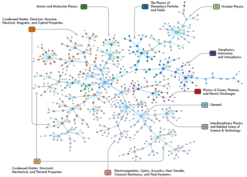
Figure 5: The maximum spanning tree of the PACS network of 2009.

Mesoscopic structure

The Maximum Spanning Tree

We now shift our focus from micro-dynamics towards the mesoscopic level and begin by illustrating the structure of the PACS network with the help of its maximum spanning tree (MST). The MST is a tree connecting all nodes of the network while maximizing the sum of link weights; such trees can be used to explore structural features in the data (see, e.g., OnnelaMST ). Figure 5 displays the MST for the PACS network of the year 2009 (874 nodes). Some structural features are apparent: first, as expected, PACS codes belonging to the same broad categories are frequently connected in the MST; however, there is mixing as well, especially in the central parts of the tree. Second, the MST reflects the underlying cluster structure of the network. There appears to be a branch that is well separated from the rest, containing fields related to high-energy physics: Physics of Elementary Particles and Fields, Nuclear Physics, and Geophysics, Astronomy and Astrophysics. The rest of physics displays more mixing in the MST, the hub nodes being frequently related to General Physics, Optics, and Condensed Matter.

$k^{s}$-shell analysis

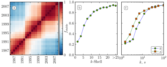
Figure 6: (a) Matrix showing the correlation coefficient between the $k^{s}$-shell indices of the PACS codes for different years. The fraction of the stable PACS codes that have remained present since their introduction as a function of its (b) $k^{s}$-shell index. (c) degree and number of appearance.

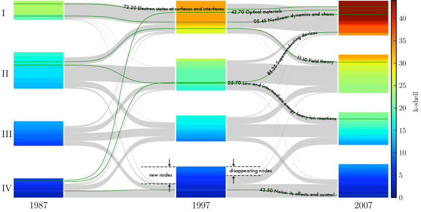
Figure 7: Evolution of the $k^{s}$-shell indices of the PACS codes and the flows between $k^{s}$-shell regions between the years 1987, 1997, and 2007. The PACS codes for each year are divided into four different categories according to their $k$-shell index (indicated by the color). The size of the block indicates the number of codes in that category, and the widths of the shaded areas correspond to the fraction of migrating codes. The green lines show $k^{s}$-shell trajectories for some specific PACS codes as examples.

Although the minimum spanning tree visualization of the network provides some overview on the structural organization of the relations between the different subfields of physics, it neither indicates the significance of the nodes forming the core of the network nor gives us any information regarding the temporal evolution of the structure. For a better and more detailed understanding, we perform $k$-core analysis Bollobas ; Seidman ; Carmi07 ; KitsakNP2010 of the evolving PACS network by decomposing the network for each year into its $k^{s}$-shells (see Methods), such that a high $k^{s}$-shell index of a node reflects a central position in the core of the network.

First, we want to establish that the $k^{s}$-shell indices of the PACS codes are relatively stable over time and are thus suitable for analysis. To do this we determine the correlation coefficients between the $k^{s}$-shell indices of all the PACS codes and between different years. In Fig. 6 (a) the correlation coefficient between different pairs of years are represented in terms of a matrix with the color of each cell representing the corresponding correlation value. The coefficient has a high value for neighboring years, so that changes in the shell indices of nodes appear gradual over time rather than randomly. Thus, the nodes having high or low $k^{s}$-shell index for year $t$ are more likely to retain their index for the subsequent year $t+1$. Furthermore, the correlation matrix shows a block diagonal structure, indicating higher correlations for three periods, 1985-1992, 1993-2000 and 2001-2009. For analysis of $k^{s}$-shell regions (see below), we pick one network corresponding to each of these periods. The $k^{s}$-shell indices of PACS codes are also related to their stability. We define a node as stable if it has been in use each year after its introduction. Fig. 6 (b) shows the fraction of stable nodes calculated over the entire period 1985-2009 as a function of the $k^{s}$-shell index; it is evident that the higher the order of the $k^{s}$-shell (and thus, the closer it is to the nucleus of the network), the larger is the fraction of stable nodes. Note that, as the $k^{s}$-shell index of a node is related to its degree and strength, nodes that have high degree or strength are also less likely to get deleted and are more stable.

For studying the time evolution of the $k^{s}$-shells, we use the alluvial diagram method Rosvall10 . We divide the PACS codes into four categories based on their $k^{s}$-shell indices by dividing the range of $k^{s}$ values into four groups of approximately equal sizes. Thus Region I contains codes that are in the core of the network ($k^{s}\in[\frac{3}{4}k_{\max}^{s},k_{\max}^{s}]$), and Regions II, III, and IV contain nodes with increasingly lower $k^{s}$-shell indices. The colored blocks of the alluvial diagram in Figure 7 show the different regions for three different years, with the size of each block representing the number of PACS codes in the respective region. The sizes are increasing with time, indicating an increase in the number of PACS codes. Furthermore, the maximum shell index $k^{s}_{\mathrm{max}}$ has increased with time, as indicated by the color of the $k^{s}$-shell indices for different years.

The shaded areas joining the $k^{s}$-shell regions represent flows of PACS codes between the regions, such that the width of the flow corresponds to the fraction of nodes. The total width of incoming flow is less than the width of the corresponding region, because the rest is made up by new PACS codes entering the network. Likewise, the gap between the width of the block and total outgoing flow corresponds to discontinued PACS codes. Here, it is seen that the core of the network, Region I, is remarkably stable compared to the peripheral Region IV that displays a high turnover of codes. Nodes that are in the core of the network are highly likely to remain so, whereas peripheral nodes frequently either disappear or migrate towards the core. Furthermore, a high fraction of new nodes first appear in the peripheral region.

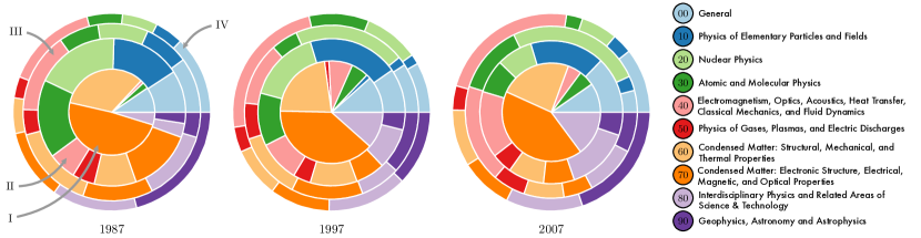
Figure 8: Multi-level pie chart for year 1987,1997 and 2007 showing the composition of each of the PACS $k^{s}$-shell regions (I-IV), such that the colors represent the first level of the PACS hierarchy.

Next, we consider how the different branches of physics are positioned with respect to the core-periphery organization of the PACS network and how their position has changed over time. Figure 8 displays multi-level pie charts for three different years, where each level of the chart represents one of the $k^{s}$-shell regions as above. The innermost layer represents Region I, followed by Region II, Region III, and finally the outermost layer represents the peripheral Region IV. For each layer, we show the fraction of level-3 PACS codes belonging to the different branches of physics as indicated by their first hierarchical PACS level.

The pie chart for the year 1987 shows that the core region I consists mostly of General Physics and Condensed Matter (PACS categories 00, 60 and 70), with a small contribution from categories 30 (Atomic and Molecular Physics), 40 (Electromagnetism etc), and 80 (Interdisciplinary Physics). In all other regions, all branches of physics are present. For the network structure of 1997, we see that the contributions of PACS categories 30, 40, and 80 have increased in the core region. Looking at the pie chart for the year 2007, we see that Interdisciplinary Physics (80) has taken over an even larger fraction of the core. The three main groups in the core are the two Condensed Matter categories (60, 70) and Interdisciplinary Physics (80). At the same time, it is seen that Nuclear Physics (20) has been moving towards the periphery, mainly contributing to Region III; this is in line with its position in the MST of Fig. 5. Thus, between 1987 and 2009, we see that Condensed Matter and General Physics have retained their position in the very core of physics, while Interdisciplinary Physics has been steadily moving towards the core, and Nuclear Physics has migrated towards the periphery. Furthermore, Physics of Elementary Particles and Fields (10) and Astrophysics (90) have retained their relative core position during this period. Note that if the above pie charts are calculated on the basis of the total number of papers for each PACS code (see Supplementary Information), no clear evolution can be observed, as the codes are more homogeneously distributed in the regions. This indicates that within each hierarchical level-1 category, there are level 3 PACS codes with highly varying volumes of publication activity and this volume does not directly correspond to the position of the code in the network.

Discussion

We have studied the evolution of physics research in terms of interconnections between its subfields from 1985 to 2009. We have shown that for yearly networks constructed from PACS codes, although there are apparent dynamical changes in the network, the key statistical distributions display remarkable stationarity. The average number of links per code and average link weight show a steady increase, indicating increased connectivity between different subfields of physics. In particular, the rate of link formation between subfields that are distant in the PACS hierarchy has increased, pointing out a clear trend of increased interdisciplinarity within physics where its different branches are becoming increasingly interlinked. This evolution does not appear random or uncorrelated; rather, within the branches there are subfields that are joined together in clusters, and there is a tendency where subfields in such clusters get connected through new links or new intermediate subfields with a high rate. The “mesoscopic” or intermediate-scale analysis of the network suggests an evolution towards increasing interdisciplinarity in physics, and a detailed study of the properties of such growing clusters would likely provide important insights into the evolution of physics.

At the mesoscopic level of the network, $k$-shell decomposition analysis reveals some large-scale trends within physics discipline: the nodes participating to the core of the network display the highest probability of survival, whereas the peripheral region displays the largest turnover associated with the discontinuations of older PACS codes and the appearance of new ones, as well as, their migration towards the core. The nodes that are in the core have a large number of connections to a large number of other nodes, and thus a high $k$-shell index can be taken as indicative of the importance of a PACS code compared to the “rest” of physics. With this interpretation it is natural that such high-$k$-shell subfields of high importance are also subfields of high stability. In our data, the core of the network has been dominated by those PACS codes that belong to the main branches of Condensed Matter and General Physics for the entire period under study. However, we also note that there is an important trend of the PACS codes belonging to Interdisciplinary Physics to steadily migrate towards the core, so that at present these already occupy a significant fraction of the core.

In conclusion, there has been an increase in the interdisciplinarity within physics, as indicated by the evolution of interconnections between different branches of physics. In addition there is an increase in the importance of Interdisciplinary Physics that also has connections to fields outside physics, as indicated by its share of the core in the PACS network. Although it may be easy to identify candidate drivers for this evolution, like the availability of vast amounts of digital data in several areas (e.g., financial markets, social systems) and an increasing number of problems requiring specialists from several fields within and outside physics (e.g., problems related to energy, climate, and biophysics), assessing their importance is beyond the scope of this study. It would be especially interesting to see how the availability of research grants in different sub-fields of physics correlate with our observations, and whether the evolution of physics follows the amount of funding available for its sub-areas or vice versa. This would require data about science funding collated from many sources. In addition, the PACS codes represent only one possible way to define the subfields of physics. Furthermore, there may be delays between developments in physics and respective changes in the PACS hierarchy. Nevertheless, we feel that it would be very interesting to compare our results with a study of the network of inter-relations between physics sub-fields constructed by using some other data than the PACS codes and recent methods such as community structure analysis of citation or co-authorship networks used to define the subfields.

Methods

Data description: A PACS code contains three elements: a pair of two-digit numbers separated by “.” and followed by two characters that may be lower- or upper-case letters or “$+$” or “$-$” signs. The first digit of the first two-digit number denotes the main category out of the 10 broad categories specified at the first level and the second digit gives the more specific field within that category. The second two-digit number specifies a narrower category within the field given by the first two digits. The last two characters may specify even more detailed categories up to the fifth level of hierarchy. As an example, in the PACS code 05.45.-a, the first digit “0” indicates “General”, adding the second digit “05”, denotes “Statistical physics, thermodynamics, and nonlinear dynamical systems” and 05.45.-a indicates “Nonlinear dynamics and chaos”; the “-” sign denotes the presence of one more level of hierarchy. Our source data comes in the form of the PACS codes of all published articles in Physical Review (PR) journals APS of the American Physical Society from 1985 till the end of 2009. In this study we use the PACS codes up to the third level of hierarchy, i.e., only the first four digits of the PACS codes. This is a good choice for longitudinal analysis: at the third level of hierarchy, the PACS codes represent the subfields of physics well and all PACS codes that have been listed in the papers extend at least to this level. Furthermore, there are more fluctuations in the deeper levels – the PACS codes change over time, as the classification scheme is regularly revised by AIP.

Network construction: For constructing the networks, we consider the individual PACS codes as nodes, such that links between them indicate that they have appeared in the same article. In order to follow the time evolution of this system, we create yearly aggregated networks by considering all articles published in a given year. We then extract the largest connected components (LCC) for all the yearly aggregated PACS networks; all network properties in this paper have been calculated for LCCs. For all years, the LCC’s correspond to almost the whole network ($>99.5\%$).

The weight of the link between the PACS code nodes $i$ and $j$ is defined as $w_{ij}=\sum_{p}\frac{1}{n_{p}-1}$, where the sum runs over the set of papers in which the PACS codes $i$ and $j$ appear together, and $n_{p}$ is the number of PACS codes used in paper $p$. This ensures that the strength of each node, $s_{i}=\sum_{j}w_{ij}$, equals the number of articles where the PACS code has been listed Newman01a (excluding articles with single PACS codes that are not part of the network).

Spearman rank correlation, and dissimilarity coefficient: If $r_{1\dots N}^{t}$ represent the degree (strength) ranks of the PACS codes for year $t$, then the Spearman rank correlation $C^{S}$ between the years $t$ and $t^{\prime}$ is defined as

$$C^{S}_{tt^{\prime}}=\frac{\sum_{i}[r_{i}^{t}-\langle r^{t}\rangle][r_{i}^{t^{\prime}}-\langle r^{t^{\prime}}\rangle]}{\sqrt{\sum_{i}[r_{i}^{t}-\langle r^{t}\rangle]^{2}\sum_{i}[r_{i}^{t^{\prime}}-\langle r^{t^{\prime}}\rangle]^{2}}},$$ (1)

where $\langle\dots\rangle$ represents the average over all nodes. From $C^{S}$ we calculate the dissimilarity coefficient $\zeta\equiv 1-(C^{S})^{2}$, where $\zeta\in[0,1]$, with low values indicating that the rank of the individual nodes remain invariant over time Kossinets06 .

Weighted overlap: In a unweighted network, the overlap is used to determine the similarity in the neighborhood of two nodes Onnela07 . However, if the network is weighted and the link weight distribution is heterogeneous, one should put more significance on links having large weights. In order to do this we define the weighted version of the neighborhood overlap $O_{ij}^{w}$ between nodes $i$ and $j$ as

$$O_{ij}^{w}=\frac{W_{ij}}{s_{i}+s_{j}-2\times w_{ij}-W_{ij}}$$ (2)

where $W_{ij}=\sum_{k\in\Lambda_{i}\cap\Lambda_{j}}(w_{ik}+w_{jk})/{2}$ and $\Lambda_{i}$ denotes the neighborhood of node $i$. Thus, $O_{ij}^{w}=0$ if the two nodes $i$ and $j$ have no common neighbors, and $O_{ij}^{w}=1$ if all of their strength is associated with links to common neighbors (except for the weight of the link joining $i$ and $j$, if any).

$k$-core analysis: We start by recursively removing nodes that have a single link until no such nodes remain in the network. These nodes form the 1-shell of the network ($k^{s}$-shell index $k^{s}=1$). Similarly, by recursively removing all nodes with degree 2, we get the 2-shell. We continue increasing $k$ until all nodes in the network have been assigned to one of the shells. The union of all the shells with index greater than or equal to $k^{s}$ is called the $k^{s}$-core of the network, and the union of all shells with index smaller or equal to $k^{s}$ is the $k^{s}$-crust of the network (see also Supplementary Information).

Author Contributions

All authors designed the research and participated in the writing of the manuscript. RKP collected the data, analysed the data and performed the research.

Additional Information

Competing financial interests

The authors declare no competing financial interests.

Supplementary Information

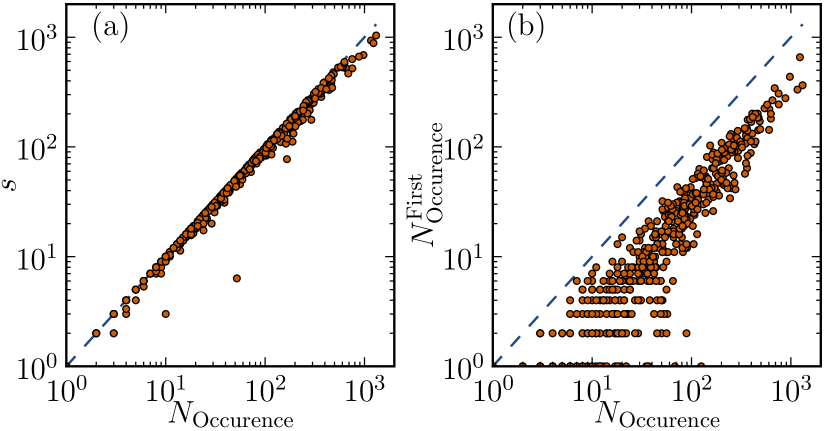
Figure 9: The number of times a PACS code has appeared in articles against (a) the node strength and (b) the number of times it has appeared as the primary code. The dashed lines show a linear dependence where the quantities are always equal. The plots are for year 2009, while data for other years indicate qualitative similarity.

Papers with single PACS codes; primary and secondary codes

For our analysis, we have ignored all papers with a single PACS code. Such papers are rather rare, as can been seen by plotting the strengths of PACS-code nodes in our networks (where single-PACS-code papers are not included) against the true number of papers where their PACS codes have appeared, using the entire data set [Fig. 9 (a)]. It is evident that these two quantities are very similar to each other.

It may also be possible that some of the PACS codes frequently appear as the primary (first) PACS code in an article, and could thus be considered more important than codes that appear mainly as secondary codes. In order to check this, in Figure 9 (b) we plot the total number of appearances of a PACS code against the number of times it has appeared as the primary code. Although there are some PACS that mainly appear as secondary code, e.g., “27.10-Properties of specific nuclei listed by mass ranges $A\leq 5$”, “02.70-Computational techniques; simulations”, etc., most of them do appear both as primary as well as secondary code.

Evolution of network properties

As seen in the main paper, the average degree, $\langle k\rangle$, of PACS networks increases linearly [Fig.1 (c) of main paper]. As a result, the average path length in these networks, $\langle\ell\rangle$, decreases linearly over this period [Fig. 10 (a)]. These features indicate that more papers joining different sub-fields of physics are appearing, leading to an increase of connectivity between them. However, the clustering coefficient of the network turns out to be constant over this period [Fig. 10 (b)], suggesting that the local connectivity of the networks remains almost constant compared to the global connectivity.

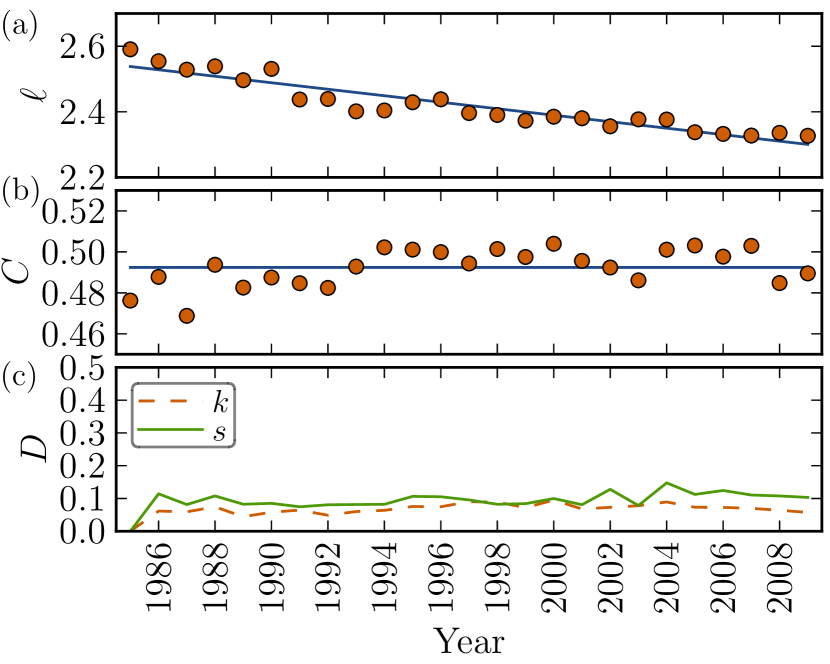
Figure 10: Time evolution of the (a) average path length $\ell$ and (b) the clustering coefficient $C$ of the PACS network with time. The solid line in (a) indicates a a linear decrease of $0.01$ in $\ell$. The line in (b) shows that clustering fluctuates at values around $C=0.49$ throughout the period of study. (c) The Kolmogorov-Smirnov statistics, $D$, comparing the degree and the strength distributions of the year 1985 with the distributions of subsequent years, indicating stationarity.

To quantify the similarity between the degree distributions of the PACS networks of different years, we measure the Kolmogorov-Smirnov statistics Massey51 $D$ of the degrees of year 1985 with the corresponding distributions of the subsequent years. Figure 10 (c) indicates that the distributions do not change much over time, as $D$ remains at a roughly constant, low value over this period. Repeating the above analysis with strength distributions reveals the same behavior. In Table 1 we show the KS distance as well the statistical significance (p values) between the degree (and strength) distribution across different years (those shown in Fig. 2 of the main paper). If the KS distance is small or the p-value is high, then we cannot reject the null hypothesis that the distributions of the two samples are the same. We found that one cannot reject the hypothesis that all the degree distribution in Fig. 2 (a) of the main paper are similar to each other ($p>0.15$). However, there is more variation across the strength distributions. For example, we found that the distribution of 1985 is different from 2009 ($p<0.01$). However, for other distributions one cannot reject the hypothesis that the distributions are similar ($p>0.05$).

Properties	Year	1993	2001	2009
Degree	1985	0.06 (0.36)	0.07 (0.18)	0.06 (0.35)
	1993		0.04 (0.63)	0.06 (0.33)
	2001			0.05 (0.31)
Strength	1985	0.08 (0.08)	0.08 (0.07)	0.10 (0.01)
	1993		0.07 (0.09)	0.06 (0.27)
	2001			0.06 (0.21)

Table 1: Kolmogorov-Smirnov (KS) test to assess whether the distributions of different years differ significantly. If the KS distance is small or the p-value is high, then we cannot reject the null hypothesis that the distributions of the two samples are the same.

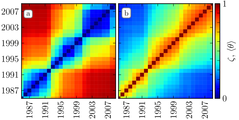
Figure 11: (a) The dissimilarity coefficient $\zeta_{tt^{\prime}}$ between the node degree ranks of different years. A small value of $\zeta$ for any two subsequent years indicates that individual node degree ranks for a given year do not change much with respect to the corresponding value of immediate next year. However, this correlation clearly decreases with time. Further, the blocks in $\zeta_{tt^{\prime}}$-matrix indicates that the ranks of node degrees as well as strengths are highly correlated between 1985-1992, 1993-2000 and 2001-2009, whereas between these regions the correlation is low. The corresponding $\zeta_{tt^{\prime}}$-matrix for strength ranks of nodes behaves similarity. (b) Plot of the average Tanimoto coefficient $\langle\theta\rangle_{tt^{\prime}}$ which shows that the weighted network structure remains rather similar for nearby years.

Although the shapes of the degree and strength distributions remain same, the degrees and strengths of the individual nodes do vary in time. Fig. 11 (a) shows the dissimilarity coefficient matrix $\zeta_{t,t^{{}^{\prime}}}$ calculated from the rank-correlation matrix $C_{S}$ for node degrees between all pairs of years $t$, $t{{}^{\prime}}$ (see Methods). As expected, we observe that the rank order is fairly similar for consecutive years and this similarity decreases with time. However, the matrix also shows the presence of a block structure of high similarity during the periods 1985-1992, 1993-2000 and 2001-2009. The block structure suggests that the degree ranks of the PACS were more stable during these periods, and that there were major changes from one period to another. To find whether only the characteristics of individual nodes have changed at these points or whether there are changes in network structure, we consider the similarities between local neighborhoods of nodes for different years. We quantify this with the Tanimoto coefficient, which is a weighted extension of the Jaccard coefficient, defined as

$$\theta_{ii}(tt{{}^{\prime}})=\frac{\sum_{j}w_{ij}(t)w_{ij}(t{{}^{\prime}})}{\sum_{j}\left[w_{ij}^{2}(t)+w_{ij}^{2}(t^{{}^{\prime}})-w_{ij}(t)w_{ij}(t{{}^{\prime}})\right]},$$ (3)

where $w_{ij}(t)$ and $w_{ij}(t{{}^{\prime}})$ are the weights of the links between nodes $i$ and $j$ for the years $t$ and $t{{}^{\prime}}$, respectively. We then measure the overall neighborhood similarity of the networks for different years by considering the weighted average over nodes

$$\langle\theta\rangle(tt{{}^{\prime}})=\frac{\sum_{i}[s_{i}(t)+s_{i}(t{{}^{\prime}})]\theta_{ii}(tt{{}^{\prime}})}{\sum_{i}[s_{i}(t)+s_{i}(t{{}^{\prime}})]}$$ (4)

where $s_{i}(t)$ and $s_{i}(t{{}^{\prime}})$ are the strengths of node $i$ for the years $t$ and $t{{}^{\prime}}$, respectively. A high value of $\langle\theta\rangle$ indicates that the network structure (including link weights) is relatively invariant. The similarity matrix $\langle\theta\rangle_{tt{{}^{\prime}}}$ is shown in Fig. 11 (b); again, the networks of consecutive years appear rather similar. Further, a block structure is evident, exhibiting an increased network similarity for the above periods.

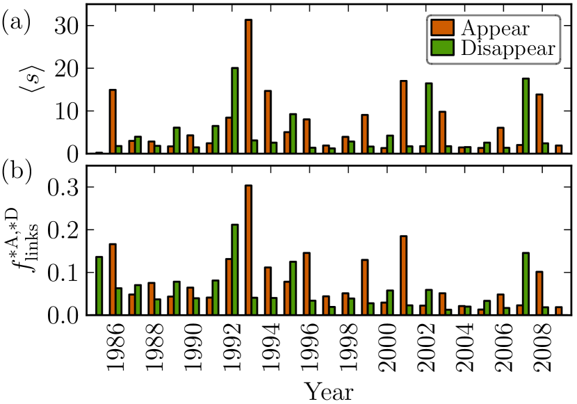
Figure 12: (a) Average strength of the appearing and the disappearing nodes. (b) Fraction of links to and between appearing (disappearing) nodes as compared to the total number of appearing (disappearing) links in a given year.

To determine the reason behind this observation, we consider the appearing and disappearing nodes. The average strengths of nodes appearing in the years 1986, 1993, 2001 and 2008 have been higher compared to other years [Fig 12 (b)]. Further, the average strengths of nodes disappearing in the years 1992, 2002 and 2007 are also relatively high. This means that many important PACS codes appeared and disappeared during these years. Next, we focus on the appearing and disappearing links in each year. We have previously observed in [Fig.1 (d) of main paper] that roughly same fraction of links appear and disappear every year. However, the ratio of links to and between the appearing nodes as compared to the total number of appearing links in a given year, $f_{\mathrm{links}}^{\mathrm{*A}}=\sum_{i\in{\mathrm{Appear}}}k_{i}/N_{\mathrm{links}}^{\mathrm{A}}$ fluctuates with time. Similarly, ratio of links to and between the disappearing nodes (just before they disappear) as compared to the total number of disappearing links in a given year, $f_{\mathrm{links}}^{\mathrm{*D}}=\sum_{i\in{\mathrm{Disappear}}}k_{i}/N_{\mathrm{links}}^{\mathrm{D}}$ also varies with time. Fig 12 (b) shows that in years, 1986, 1993 and 2001 more newly appearing links were connected to newly born nodes as compared to the other years, while in years 1985, 1992 and 2007 more links disappeared due to nodes disappearing. Thus, there is relatively more change in network structure during these years due to the high degree of appearing and disappearing nodes. We found that many of these newly appearing PACS codes were introduced to refine the sub-field and thus replace an existing code that did not represent the field well whereas others were introduced as a result of discovery of new concepts.

Comparison of empirical network with null models

We have compared the structural properties of the PACS network with a randomized ensemble of networks where the PACS codes are reshuffled among papers. This provides a null model giving insight into whether the observed properties are expected by chance as a consequence of the constraints inherent in the system. In Table 2, we report the number of nodes $N$, the number of links $L$, clustering coefficient $C$, the average path length $\ell$ and the average weight of the links $w$ of the network for years 1985, 1993, 2001, 2009 and the corresponding randomized versions that are obtained by randomly shuffling the PACS codes across papers. We first observe that there are more links in the randomized network compared to the empirical network because the PACS pairs that appear frequently in the empirical network are now less likely to be seen together. Instead, each member of the pair are more likely to appear together with other codes, forming new links. This leads to an increase in the clustering coefficient, decrease in the average link weight and also decreases the average path length.

Year	$N$	$C$	$C^{\mathrm{rand}}$	$L$	$L^{\mathrm{rand}}$	$\langle w\rangle$	$\langle w\rangle^{\mathrm{rand}}$	$\ell$	$\ell^{\mathrm{rand}}$
1985	438	0.48	0.56$\pm$0.009	4688	9627$\pm$41	1.53	0.79$\pm$0.003	2.6	2.1$\pm$0.009
1993	503	0.49	0.65$\pm$0.006	7604	16193$\pm$56	1.89	0.95$\pm$0.003	2.4	2.0$\pm$0.006
2001	614	0.50	0.65$\pm$0.005	10797	23438$\pm$66	1.79	0.89$\pm$0.003	2.4	2.0$\pm$0.005
2009	620	0.49	0.67$\pm$0.005	12826	29294$\pm$65	1.99	0.95$\pm$0.002	2.3	1.9$\pm$0.004

Table 2: Comparison of the properties of the real network with the randomized null model. The network for the null models are created from an ensemble where the PACS codes are reshuffled among the papers. The properties of the random network are averaged over 100 different realizations.

This randomization process also destroys the hierarchical structure of the network. In Table 3, we show the fraction of links that connect nodes at different hierarchical distances ($h=0,1,2$). We compare it with the corresponding fraction in the null model. As expected, most of the links now connect nodes that are hierarchically different and very few links connect nodes that are hierarchically similar. For example, in 2009, 61% of links in the empirical network connect nodes that are dissimilar (h=0), which is much lower that the 87% of the links that appear in the null model. Furthermore, 12% of the links are between similar nodes (h=2), which is much larger that 2% of such links in the randomized network. This loss of hierarchical and modular structure can be seen in the minimum spanning tree of the randomized version of the PACS network of 2009 [Fig 13].

Year	$f_{\mathrm{link}}^{h=0}$	$f_{\mathrm{link}}^{h=0}|_{\mathrm{rand}}$	$f_{\mathrm{link}}^{h=1}$	$f_{\mathrm{link}}^{h=1}|_{\mathrm{rand}}$	$f_{\mathrm{link}}^{h=2}$	$f_{\mathrm{link}}^{h=2}|_{\mathrm{rand}}$
1985	0.52	0.85$\pm$0.003	0.34	0.13$\pm$0.002	0.14	0.02$\pm$0.0012
1993	0.57	0.85$\pm$0.002	0.30	0.12$\pm$0.002	0.12	0.02$\pm$0.0008
2001	0.60	0.86$\pm$0.002	0.28	0.11$\pm$0.001	0.13	0.02$\pm$0.0006
2009	0.61	0.87$\pm$0.001	0.28	0.11$\pm$0.001	0.12	0.02$\pm$0.0005

Table 3: Comparison of the fraction of links between nodes in different hierarchical level in the real network with the randomized null model. The network for the null models are created from an ensemble where the PACS codes are randomly shuffled among the papers. The properties of the random network are averaged over 100 different realizations.

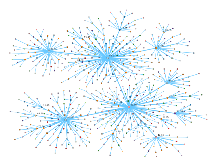
Figure 13: The maximum spanning tree of the randomized version of the PACS network of 2009. Compared to the empirical network, there is a clear lack of hierarchical structure, as most nodes are connected to a small number of high-degree nodes. Further, the modularity in terms of frequent connections between nodes in similar categories is also lost.

Microdynamics of new links between dissimilar and similar nodes

In [Fig.3 of the main paper], we have shown that a substantial and increasing fraction of new links connects nodes that belong to different level 1 PACS categories ($h=0$), whereas the fraction of new links to similar $h=2$ nodes is decreasing with time. However, because of the hierarchical nature of the PACS tree, there are many more node pairs with $h=0$ than with $h=2$, and thus even randomly placed links would more often fall between $h=0$ nodes. Thus, in theory, the increasing number of new links joining $h=0$ nodes might be explained by the increasing number of PACS codes. In order to verify the existence of a real trend, we have plotted the number of new links between $h=0$ or $h=2$ nodes, $N^{A}$, normalized by the corresponding number $N^{A}_{\mathrm{rand}}$ in a randomized null model where all the $N^{A}$ links are placed randomly. Fig. 14 shows that the increasing trend for new links between $h=0$ nodes is present even with this normalization, and the likelihood of new links connecting dissimilar PACS branches is thus increasing with time.

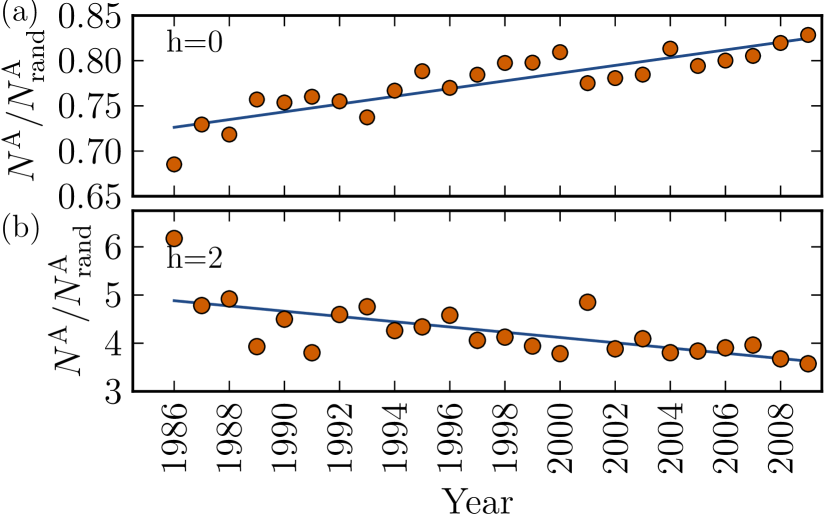
Figure 14: The number of newly appearing links $N^{A}$ falling between PACS codes that are dissimilar $h=0$ or similar to the 2nd level of the PACS hierarchy ($h=2$), normalized by the expected number $N^{A}_{\mathrm{rand}}$ in a null model where all new links are placed randomly in the network.

Microdynamics of new nodes

In the main text of the paper we have explained the method to determine similar connectivity pattern for disappearing PACS codes. We can perform a similar analysis focusing on PACS codes that are newly introduced. For each of the newly introduced PACS code $i$, we find their peak years $t^{\ast}$ with the highest number of published papers and determine the network neighborhood $\Lambda_{i,t^{\ast}}$ corresponding to the peak year. We then calculate the overlap of this neighborhood with the neighborhoods of all nodes in the network at year $t_{i}-1$, where $t_{i}$ is the year when $i$ appeared. We then choose the node $j$ that has the maximum overlap with $\Lambda_{i,t^{\ast}}$, and thus has the most similar link pattern with $i$ at its peak. As in the case of discontinued PACS, we found that as the maximum strength of the introduced PACS codes increases, the maximum overlap also increases. Further, it is seen that only $\sim 10\%$ of new codes appear to replace discontinued codes, and thus the majority of new codes seem to correspond to emerging new subfields [Fig.4 (h) of main paper].

Properties of unstable nodes and links

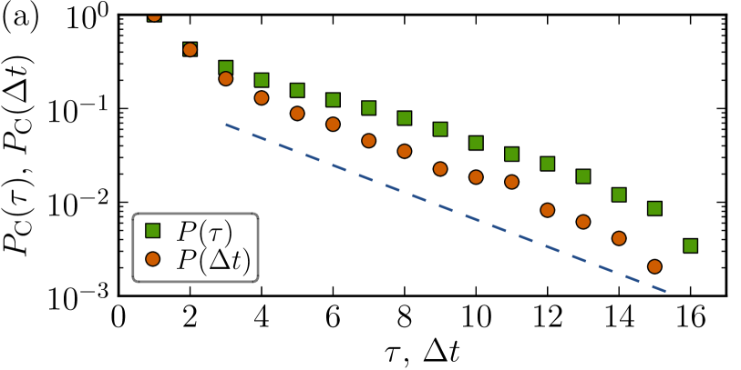
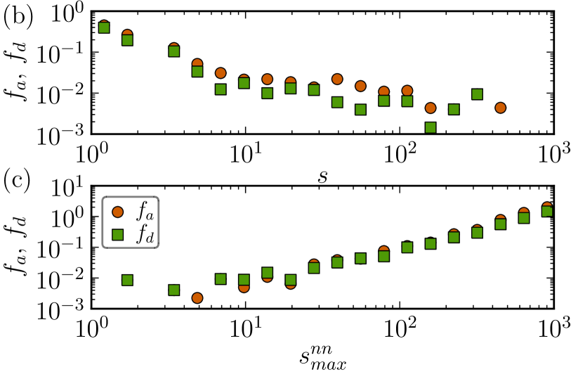
Figure 15: Properties of appearing and disappearing nodes. (a) Distribution of the time of existence $\tau$ and the period of absence $\Delta t$ of the transient nodes (nodes that both appear and later disappear). The dashed line indicates an exponential decay, $\sim\exp(-t/3)$. The fraction of appearing and disappearing nodes of a given (b) strength $s$ and (b) maximum strength of neighbors $s_{\mathrm{max}}^{\mathrm{nn}}$, as compared to other nodes in the network.

The PACS network displays turnover in terms of both nodes and links. Here we focus on those nodes and links that appear (i.e. are present at year $t$ but not at $t-1$) or disappear i.e. are present at $t$ but not at $t+1$) during the period of study (1985-2009). As seen in [Fig.1 (d) of main paper], the percentage of appearing and disappearing nodes is between 5%-10% per year. We first focus only on transient nodes that appear and later disappear during the observation period. To characterize the transient nodes, we consider the time for which they are continuously present, $\tau$. As transient nodes may reappear in the network after their disappearance, we also measure the time of their absence, $\Delta t$. The distributions of both quantities decay exponentially, $P(\tau)\propto\exp(-\alpha\tau)$ and $P(\Delta t)\propto\exp(-\beta\Delta t)$, with exponent $\alpha\sim\beta\sim 1/3$ [Fig. 15(a)]. This means that nodes that are present (absent) for three consecutive years are $1/e$ times less likely to disappear (appear).

Next, we compare the properties of all nodes that appear or disappear during the observation period with other nodes in the network. We define $f_{a}(s)$ as the fraction of nodes of strength $s$ that appear during the period of observation,

$$f_{a}(s)=\frac{\sum_{t}N_{t}^{a}(s)}{\sum_{t}N_{t}(s)},$$ (5)

where $N_{t}(s)$ is the number of nodes with strength $s$ at time $t$ and $N_{t}^{a}(s)$ is the number of nodes with strength $s$ that appear between $t$ and $t+1$. We similarly define $f_{d}(s)$, the fraction of nodes of strength $s$ that disappear during the period of observation Gautreau09 . Most of these appearing and disappearing nodes have low strength, indicating they were used in very few papers at the time of appearance or just before disappearance [Fig. 15 (b)]. However, a few nodes with high strength appear or disappear with non-negligible probability. As the degree and the strength of the nodes are related, the $f_{a}$ and $f_{d}$ behave very similarly with the node degree (not shown). When measuring $f_{a}$ and $f_{d}$ as a function of the maximum degree of the node’s neighbor, it is seen that appearing and disappearing nodes are mainly connected to hubs [Fig. 15 (c)]. Thus, most of the appearing nodes get connected to nodes of high strength and degree and the neighbors of high-strength and high-degree nodes are more likely to disappear, as compared to the neighbors of low strength and non-hub nodes.

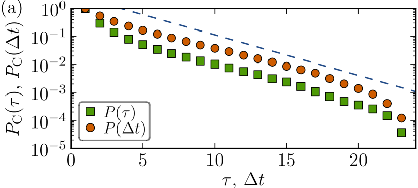
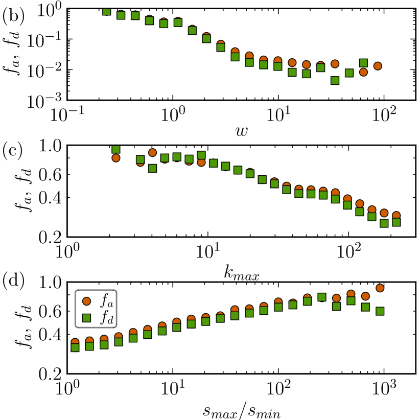
Figure 16: Properties of appearing and disappearing links. (a) Distribution of the time of existence and period of absence for the transient links (those which appear as well as disappear). The line indicates an exponential decay, $\exp(-t/3)$. Fraction of appearing and disappearing links of a given (b) link weight $w$, (c) maximum degree of the connecting nodes $k_{\mathrm{max}}$ and (d) ratio of strength of nodes connected by the link, $s_{\mathrm{max}}/s_{\mathrm{min}}$, as compared to the overall links in the network.

Next, we focus on the links that appear or disappear during our period of observation; as seen in [Fig.1 (d) of main paper], about 40 percent of links appear and a similar number of them disappear every year. We first consider only the transient links that appear and then disappear during the period of observation. In Fig. 16 (a) we show the distribution for the period for which they were present continuously, $\tau$, and the period of absence, $\Delta t$, defined as for the nodes. Again, both distributions decay exponentially with an exponent of $-1/3$, similarly to the behavior observed for transient nodes. This suggest that most of these links appear or disappear as new nodes are introduced to the network or nodes leave the network, respectively. This behavior is different from the node and link dynamics of air transportation network Gautreau09 where the nodes are mostly stable and the distribution of link’s absence and presence decays as a power law. This means that in the PACS network links that are absent for a long time are much less likely to reappear, and links that are present for a considerable period are much less likely to disappear, as compared to the case in the airport network. This may be related to the economic constraints operating in the airport network that make commercially unenviable links more likely to disappear and the profitable links more likely to appear.

As we did for nodes, we also compare the properties of all appearing and disappearing links with overall properties of links.The fraction of links of weight $w$ that disappear during the time-period 1985-2009 is defined as

$$f_{d}(w)=\frac{\sum_{t}N_{t}^{d}(w)}{\sum_{t}N_{t}(w)},$$ (6)

where $N_{t}(w)$ is the number of links with weight $w$ at time $t$ and $N_{t}^{d}(w)$ is the number of links with weight $w$ that disappear between $t$ and $t+1$. The fraction $f_{a}(w)$ of links of weight $w$ that appear is defined as for the nodes. Most of the appearing and disappearing links have low weight; however, links with high weight may also appear and disappear with a non-negligible probability [Fig. 16 (b)]. We also measure $f_{a}$ and $f_{d}$ as a function of the maximum degree of the two nodes that the link connects. We find that the most of the links which appear or disappear are between non-hubs [Fig. 16 (c)]. Similarly, we measure $f_{a}$ and $f_{d}$ as a function of the ratio of the $s_{\mathrm{max}}/s_{\mathrm{min}}$ of a link, where $s_{\mathrm{max}}$ and $s_{\mathrm{min}}$ are the maximum and the minimum strength of the nodes joined by the link. Fig. 16 (d) shows that these links mostly connect nodes of heterogeneous strength.

$k^{s}$-core decomposition and $k$-crust connectivity

In Figure 17, we show the number of nodes and the size of the largest connected component (LCC) as a function of the $k$-crust from the $k^{s}$-core decomposition of the network of years 1987 and 2007. As expected, both the number of nodes and the LCC size increase with $k$-crust. For smaller $k$, the LCC and the crust sizes are different, whereas for larger $k$ the LCC becomes almost of the same size as the crust. This feature is different from some other empirically observed networks Carmi07 , where the nucleus plays a crucial role in the connectivity of the network. In most of these empirical systems, the network is in general fragmented into multiple disconnected components before the introduction of the nucleus. However, in the PACS network the crust is already almost connected even before the introduction of the nucleus. Therefore, in the PACS network, the nucleus plays a less important role; e.g., were any dynamical process of information flow to take place on the network, it would not necessarily need to pass through the nucleus.

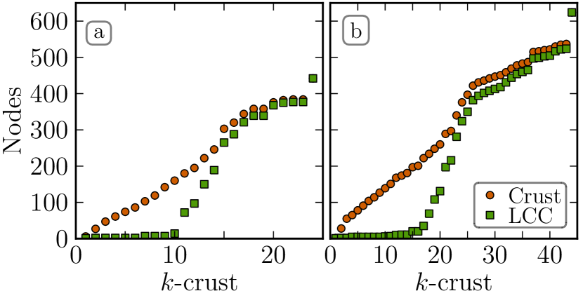
Figure 17: The number of nodes and size of the largest connected component in each of the $k^{s}$-crust for the years (a) 1987 and (b) 2007.

Evolution of publication volumes of PACS codes

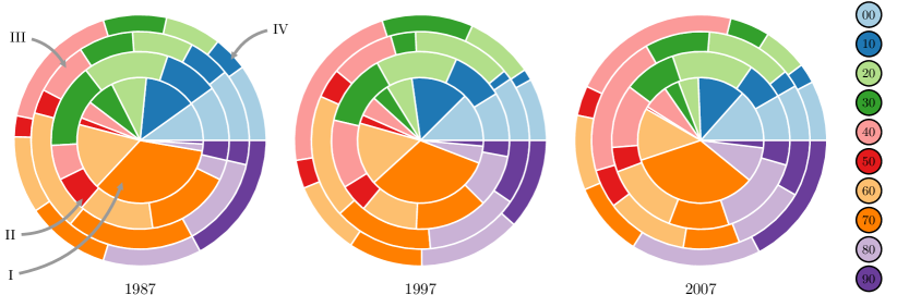
Figure 18: Multi-level pie chart for years 1987, 1997 and 2007 showing the time evolution of the publication volumes of PACS codes which are categorized according to their field they represent.

Instead of the $k$-core decomposition and the core indices of PACS codes, one could argue that the importance of a PACS code might be represented simply by the number of papers published with it. To compare with the $k^{s}$-shell analysis and the evolution of the core indices of different codes, as done in [Fig.8 of main paper], we plot a similar multi-level pie chart where the regions correspond to the numbers of papers with given PACS codes. Again, Region I contains the top 25% PACS codes, this time in terms of total publication volume, and Regions II, III, and IV PACS codes with increasingly lower publication volumes. As before we categorize the PACS codes in each of these region with the first digit of their hierarchy. Although the number of papers for a code and its $k^{s}$-shell index are related, Fig. 18 is very different from [Fig.8 of main paper]. For each year, all fields are represented in each of the four regions. This means that for all PACS categories, there are sub-categories with high publication volumes and sub-categories with low volumes. Even the subfields of “10-The Physics of Elementary Particles and Fields” and “20-Nuclear Physics” are present in the region I, whereas they appear only in the mid and peripheral shells when categorized according to their $k^{s}$-shell index. There are no clear trends, although there is small increase in the number of high-volume “80-Interdisciplinary Physics and Related Areas of Science and Technology” PACS codes.

References

- (1) Popper, K. R. The Logic of Scientific Discovery (Basic Books, New York, USA, 1959).
- (2) Kuhn, T. The Structure of Scientific Revolutions (University of Chicago press, Chicago, 1962).
- (3) Newman, M. E. J. Scientific collaboration networks. ii. shortest paths, weighted networks, and centrality. Phys. Rev. E 64, 016132 (2001).
- (4) Redner, S. How popular is your paper? an empirical study of the citation distribution. Eur. Phys. J. B 4, 131–134 (1998).
- (5) Pan, R. K. & Saramaki, J. The strength of strong ties in scientific collaboration networks. Europhys. Lett. 97, 18007 (2012).
- (6) Redner, S. Citation statistics from 110 years of physical review. Phys. today 58, 49–54 (2005).
- (7) Gautreau, A., Barrat, A. & Barthélemy, M. Microdynamics in stationary complex networks. Proc. Natl. Acad. Sci. U.S.A. 106, 8847 (2009).
- (8) http://publish.aps.org/.
- (9) http://www.aip.org/pacs/ (accessed on 01-02-2011).
- (10) Radicchi, F. & Castellano, C. Rescaling citations of publications in physics. Phys. Rev. E 83, 046116 (2011).
- (11) Massey Jr, F. The Kolmogorov-Smirnov test for goodness of fit. J Am. Stat. Assoc. 46, 68–78 (1951).
- (12) Kossinets, G. & Watts, D. J. Empirical analysis of an evolving social network. Science 311, 88–90 (2006).
- (13) Granovetter, M. The strength of weak ties. Am. J. Sociol. 78, 1360–1380 (1973).
- (14) Liben-Nowell, D., Novak, J., Kumar, R., Raghavan, P. & Tomkins, A. Geographic routing in social networks. Proc. Natl. Acad. Sci. U.S.A. 102, 11623–11628 (2005).
- (15) Onnela, J.-P., Chakraborti, A., Kaski, K., Kertész, J. & Kanto, A. Asset trees and asset graphs in financial markets. Phys. Scripta T106, 48–54 (2003).
- (16) Bollobás, B. in Graph Theory and Combinatorics: Proceedings of the Cambridge Combinatorial Conference in Honour of P. Erdős, (Academic, 1984) pp. 35-57.
- (17) Seidman, S. Network structure and minimum degree. Social Networks 5, 269–287 (1983).
- (18) Carmi, S., Havlin, S., Kirkpatrick, S., Shavitt, Y. & Shir, E. A model of internet topology using k-shell decomposition. Proc. Natl. Acad. Sci. U.S.A. 104, 11150–11154 (2007).
- (19) Kitsak, M. et al. Identification of influential spreaders in complex networks. Nature Phys. 6, 888–893 (2010).
- (20) Rosvall, M. & Bergstrom, C. T. Mapping change in large networks. PLoS ONE 5, e8694 (2010).
- (21) Onnela, J.-P. et al. Structure and tie strengths in mobile communication networks. Proc. Natl. Acad. Sci. U.S.A. 104, 7332 (2007).
Acknowledgments
Financial support from EU’s 7th Framework Program’s FET-Open to ICTeCollective project no. 238597 and by the Academy of Finland, the Finnish Center of Excellence program 2006-2011, project no. 129670 are gratefully acknowledged. We would like to thank S Sanyal and A Basu for helpful discussions.