Nonlinear Nanomechanical Resonators for Quantum Optoelectromechanics

Abstract

We present a scheme for tuning and controlling nanomechanical resonators by subjecting them to electrostatic gradient fields, provided by nearby tip electrodes. We show that this approach enables access to a novel regime of optomechanics, where the intrinsic nonlinearity of the nanoresonator can be explored. In this regime, one or several laser driven cavity modes coupled to the nanoresonator and suitably adjusted gradient fields allow to control the motional state of the nanoresonator at the single phonon level. Some applications of this platform have been presented previously Rips2012 ; Rips2013 . Here, we provide a detailed description of the corresponding setup and its optomechanical coupling mechanisms, together with an in-depth analysis of possible sources of damping or decoherence and a discussion of the readout of the nanoresonator state.

I Introduction

Substantial progress in fabricating high-$Q$ mechanical resonators with high frequencies, as well as recent success in cooling them close to the motional ground state nature08681 ; nature08967 ; nature10261 ; nature10461 ; Verhagen12 , inaugurate a new research field of manifold fundamental interest science.1156032 ; Physics.2.40 ; PhysRevLett.88.148301 . The regime of very low temperature, where a quantum mechanical description predicts only few quanta of mechanical motion, promises potential insight into some fundamental questions of decoherence, as well as various technical applications that make use the of the expected quantum behavior nnano.2009.343 ; nphys1304 ; PhysRevA.82.061804 . Fundamental questions, concerning the border between the classical (macroscopic) and the quantum (microscopic) worlds Adler17072009 , trigger a natural interest in preparing quantum states of “as large as possible” objects and demonstrating their distinct quantum behavior by appropriate measurements. See Aspelmeyer13 for a recent review.

Regarding this major goal, it is important to stress that the dynamics of a purely harmonic quantum system is analogous to its classical dynamics, in the sense that expectation values of canonical observables follow the classical equations of motion ehrenfest . Therefore, it is a common approach to introduce nonlinearities in a quantum system in order to detect quantum behavior. While there may be the possibility to achieve the strong optomechanical coupling regime Rabl11 ; Nunnenkamp11 ; nphys1707 and make use of the nonlinear nature of the standard optomechanical coupling, or to couple to a nonlinear ancilla system nature08967 ; PhysRevLett.88.148301 ; PhysRevLett.99.117203 , we propose here a different approach: the use of an optoelectromechanical system featuring a tunable mechanical nonlinearity per phonon. The latter originates from the intrinsic geometric nonlinearity of elastic systems Phys.Rev.B64_220101 ; 1367-2630-8-2-021 ; 1367-2630-10-10-105020 ; PhysRevLett.99.040404 ; PhysRevLett.101.200503 ; Dykman11 and its amount per motional quanta is enhanced with the help of electrostatic fields. This has the advantage that the linear optomechanical coupling is preserved as a control channel providing techniques as, for example, the sideband driving technique used in Rips2012 . The regime of large mechanical nonlinearity then enables new means to control the mechanical motion at the quantum level, if combined with the coupling to a high-Q optical cavity mode, as well as the application of suitable gradient fields.

The intrinsic anharmonicity in the mechanical motion of micro- and nanomechanical resonators is usually small and therefore only relevant in the regime of large oscillation amplitudes. In order to render the anharmonicity relevant for displacements at the scale of the quantum mechanical zero point motion, we propose to use electrostatic gradient forces to enhance the latter nature07932 . These forces result from the dielectric properties of the resonator material when an inhomogeneous external electric field is applied. They can be used to effectively reduce the resonator’s stiffness and therefore its resonance frequencies. In turn, this has the effect that the zero point deflection is enhanced up to an extent that the nonlinear contribution becomes important.

Using this technique, the nonlinearity per phonon can be made large enough, that distinct transitions in the mechanical spectrum can be resonantly addressed while interacting with other quantum systems. Examples are the selective sideband driving of transitions in the mechanical spectrum Rips2012 , or the resonant exchange of excitations within an array of nanoresonators via a common cavity mode Rips2013 .

In this paper, we explicitly derive the fundamental mode properties of a nonlinear mechanical resonator, subject to the aforementioned gradient forces, to obtain a suitable model for the mechanical degree of freedom. We then derive the specifics of the optomechanical coupling to a high finesse cavity and analyze possible source of damping and decoherence in detail. We also summarize different control schemes, associated with suitable laser drives for the cavity and gradient fields from the tip electrodes. Two applications of these control mechanisms have been proposed previously Rips2012 ; Rips2013 , considering state of the art experimental components. We finally discuss a readout scheme for the nonlinear mechanical resonators considered.

The remainder of the paper is organized as follows. In section II we describe the nonlinear dynamics of thin rods starting from elasticity theory and derive the resulting fundamental mode Hamiltonian. In section III we describe our approach to enhance the intrinsic mechanical nonlinearity by mode softening with gradient forces. Then we introduce the optomechanical model with several laser driven cavity modes in section IV. After introducing a possible setup for an implementation in section V, we quantitatively discuss its central physical properties, namely the optomechanical coupling mechanism in section VI, as well as potential setup specific losses in section VII. In section VIII we review some mechanisms that can be used to control the mechanical motion at the level of single phonons and which have been applied in previous works Rips2012 ; Rips2013 . Finally, in section IX we introduce methods to obtain information on the mechanical state from the output spectrum of a probe laser.

II Elasticity and fundamental mode description

The harmonic description of the transverse motion of thin rods is based on only considering the bending energy for small deflections Landau-Lifshitz . We consider here thin rods, which means that the cross-sectional dimensions, such as the radius for circular cross sections or width and depth for rectangular cross sections, are much smaller than the length $L$. We also consider the rod to be homogeneous along the longitudinal axis, here parametrized by $x\in\{0,L\}$, with constant mass line density $\mu$ and use thin rod elasticity theory. The planar deflection in the transverse direction is described by a field $y(x)$ and we consider a bridge geometry where the end points at $x=0$ and $x=L$ are fixed, i.e. $y(0)=y(L)=0$ and $y^{\prime}(0)=y^{\prime}(L)=0$. The Lagrangian within this approximation reads

$$\mathcal{L}(y(x,t))=\frac{\mu}{2}\int\mathrm{d}x\dot{y}^{2}-V_{\mathrm{b}}[y(x)]\,,$$ (1)

with a kinetic part as well as the bending energy

$$V_{\mathrm{b}}[y(x)]=\frac{1}{2}\int\limits\mathcal{F}\tilde{\kappa}^{2}(y^{\prime\prime})^{2}{\rm d}x\,.$$ (2)

Here, $\mathcal{F}=YA$ is the linear modulus of the rod given by the Young modulus $Y$ of the material times the cross-section area $A$, and $\tilde{\kappa}^{2}=\frac{1}{A}\int_{\mathrm{cross}}\tilde{y}^{2}{\rm d}A$ is the ratio between the bending and compressional rigidities and depends on the cross-sectional geometry, where $\tilde{y}$ is the in-plane coordinate within the cross-section that is directed along the deflection with origin at the neutral line, see figure 1. For a rectangular cross-section of thickness $d$, $\tilde{\kappa}=d/\sqrt{12}$, whereas for a circular cross-section with radius $R$, $\tilde{\kappa}=R/2$. For a cylindrical shell like a nanotube one finds $\tilde{\kappa}=R/\sqrt{2}$. The energy (2) results from the fact that for small curvature $y^{\prime\prime}$, the local strain inside the rod is linear with respect to the distance $\tilde{y}$ to the neutral surface (cf. Fig. 1) while the free energy density is quadratic with respect to the strain.

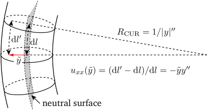
Figure 1: Section of a deflected rod. The local strain $u_{xx}$ depends on the transverse coordinate $\tilde{y}$ and on the local curvature $y^{\prime\prime}$ and determines the energy density $\tfrac{1}{2}Yu_{xx}^{2}$.

The Lagrangian (1) leads to the equation of motion

$$\mu\partial_{t}^{2}y+\mathcal{F}\tilde{\kappa}^{2}\partial_{x}^{4}y=0\,.$$ (3)

As this equation is linear in $y$ and its derivatives, it leads to harmonic dynamics characterized by the following eigenmodes

$$\phi_{n}(x)=\frac{1}{C_{n}}\bigg{[} \frac{\sin(\nu_{n}x/L)-\sinh(\nu_{n}x/L)}{\sin(\nu_{n})-\sinh(\nu_{n})}$$ (4)

$$-\frac{\cos(\nu_{n}x/L)-\cosh(\nu_{n}x/L)}{\cos(\nu_{n})-\cosh(\nu_{n})}\bigg{]}\,,$$

with frequencies $\omega_{n}=c_{\mathrm{s}}\tilde{\kappa}\left(\nu_{n}/L\right)^{2}$, where $c_{\mathrm{s}}=\sqrt{\mathcal{F}/\mu}$ is the phase velocity of compressional phonons along the rod. The $\nu_{n}$ are the roots of the transcendental equation $\cos\left(\nu_{n}\right)\cosh\left(\nu_{n}\right)\!=\!1$, with $\nu_{1}=4.73$ the smallest one. The $C_{n}$ are normalization constants chosen such that ${\mathrm{\bf max}}\left\{\phi_{n}(x)\right\}\!=\!1$. We choose this normalization so that the coefficients in a mode expansion represent the maximum amplitudes of the deflection associated to each mode. Introducing now the canonical momentum $\Pi(x,t)=\delta\mathcal{L}/\delta\dot{y}(x,t)$, as well as the expansion of the field into the modes

$$y(x,t)=\sum_{n}\phi_{n}(x)\mathcal{X}_{n}(t)\,,$$ (5)

yields the Hamilton function of a harmonic oscillator for each mode

$$\mathcal{H}_{\mathrm{lin}}=\sum_{n}\left(\frac{\mathcal{P}_{n}^{2}}{2m^{*}_{n}}+\frac{1}{2}m_{n}^{*}\omega_{n}^{2}\mathcal{X}_{n}^{2}\right)\,$$ (6)

with the deflection $\mathcal{X}_{n}$ and mode momentum $\mathcal{P}_{n}=m^{*}_{n}\partial_{t}\mathcal{X}_{n}$ for the $n$-th mode, as well as the effective mode masses $m^{*}_{n}=\mu\int_{0}^{L}\phi^{2}_{n}(x){\rm d}x$.

Corrections to this harmonic description that lead to nonlinearities originate from a stretching effect that occurs due to the deflection if the end points of the rod are fixed Phys.Rev.B64_220101 . The resulting strain leads to an additional energy

$$\frac{\mathcal{F}}{2}\frac{(L_{t}-L)^{2}}{L}\approx\frac{\mathcal{F}}{8L}\left(\int{\rm d}x(y^{\prime})^{2}\right)^{2}\,,$$ (7)

where the stretched length is $L_{t}=\int\sqrt{1+(y^{\prime})^{2}}{\rm d}x\approx L+\tfrac{1}{2}\int{\rm d}x(y^{\prime})^{2}$ with $L$ being the zero deflection length. Including this streching energy leads to a nonlinear extension of the Hamiltonian, which after inserting the modes given in Eq. (5) leads to

$$\mathcal{H}\!=\!\mathcal{H}_{\mathrm{lin}}+\frac{\mathcal{F}}{8L}\sum_{i,j,k,l}M_{ij}M_{kl}\mathcal{X}_{i}\mathcal{X}_{j}\mathcal{X}_{k}\mathcal{X}_{l}\,,$$ (8)

where $M_{ij}=\int_{0}^{L}\phi_{i}^{\prime}(x)\phi_{j}^{\prime}(x){\rm d}x$. We quantize this model by introducing bosonic mode operators $c_{n}^{{\dagger}}$ and $c_{n}$, given by

$$c_{n}=\frac{1}{2x_{\mathrm{ZPM},n}}\,\mathcal{X}_{n}+\mathrm{i}\frac{x_{\mathrm{ZPM},n}}{\hbar}\,\mathcal{P}_{n}\,,$$ (9)

where we introduced the zero point motion amplitudes $x_{\mathrm{ZPM},n}=\sqrt{\hbar/2m_{n}^{*}\omega_{n}}$ for each mode. This leads to the description

$$\mathcal{H}= \sum_{n}\hbar\omega_{n}\left(c_{n}^{{\dagger}}c_{n}+\frac{1}{2}\right)$$ (10)

$$+ \hbar\sum\limits_{ijkl}\lambda_{ijkl}^{0}\left(c_{i}^{{\dagger}}+c_{i}\right)\left(c_{j}^{{\dagger}}+c_{j}\right)\left(c_{k}^{{\dagger}}+c_{k}\right)\left(c_{l}^{{\dagger}}+c_{l}\right),$$

with nonlinearity

$$\lambda_{ijkl}^{0}=\frac{\mathcal{F}}{8L\hbar}M_{ij}M_{kl}x_{\mathrm{ZPM},i}x_{\mathrm{ZPM},j}x_{\mathrm{ZPM},k}x_{\mathrm{ZPM},l}\,.$$ (11)

As in a rigorous elasticity treatment this description arises from an adiabatic elimination of the stretching modes, the indices in Eq. (10) should run up to an $N$ corresponding to an “ultraviolet” cutoff $\omega_{N}\sim c_{\mathrm{s}}\pi/L$. The terms involving higher order modes induce small frequency shifts and nonlinear mode coupling. However, the later is found to be negligible for the parameters considered (see Appendix B) and the shift of the fundamental mode can be ignored given the additional tunable electrostatic contribution (see Section III).

Therefore we can restrict our description to the fundamental mode with $n=1$ and drop this label to get the usual Hamiltonian for the Duffing oscillator

$$H_{\mathrm{m},0}=\frac{\mathcal{P}^{2}}{2m^{*}}+\frac{1}{2}m^{*}\omega_{\mathrm{m,0}}^{2}\mathcal{X}^{2}+\frac{\beta}{4}\mathcal{X}^{4}\,,$$ (12)

where we have introduced the fundamental frequency $\omega_{\mathrm{m,0}}$ and the effective mass of the fundamental mode $m^{*}\approx 0.3965\,\mu L$. The anharmonicity is given by

$$\beta=\frac{\left(M_{11}L\right)^{2}}{2\nu_{1}^{4}\left(m^{*}/\mu L\right)}\,m^{*}\frac{\omega_{\mathrm{m},0}^{2}}{\tilde{\kappa}^{2}}\approx 0.060\,m^{*}\frac{\omega_{\mathrm{m},0}^{2}}{\tilde{\kappa}^{2}}\,.$$ (13)

In terms of phonon creation and annihilation operators $b^{{\dagger}}=c_{1}^{{\dagger}}$ and $b=c_{1}$ this Hamiltonian reads,

$$H_{\mathrm{m},0}=\hbar\omega_{\mathrm{m},0}b^{{\dagger}}b+\hbar\frac{\lambda_{0}}{2}\left(b^{{\dagger}}+b\right)^{4}\,,$$ (14)

with the nonlinearity parameter $\lambda_{0}\equiv 2\lambda_{1111}^{0}=\frac{\beta}{2}x_{\mathrm{ZPM}}^{4}/\hbar$. Here, the frequencies $\omega_{\mathrm{m},0}$ and $\lambda_{0}$ refer to fundamental mode properties that result only from the intrinsic elastic forces in the absence of any externally applied forces on the rod. As we will describe in the next section, external forces can be used to tune the resonance frequency, $\omega_{\mathrm{m},0}\rightarrow\omega_{\mathrm{m}}$, which will in turn change the zero point motion amplitude, $x_{\mathrm{ZPM}}$, and hence the nonlinearity, $\lambda_{0}\rightarrow\lambda$.

III Electric gradient fields

In this section we describe how electric fields generated by tip electrodes that are placed near the center of the doubly clamped nanobeam, see figure 2, can be employed to control its dynamical properties. In particular, inhomogeneous gradient fields can be used to enhance the nonlinearity per phonon. The later scales as $\lambda\propto x_{\mathrm{ZPM}}^{4}\propto\omega_{\mathrm{m}}^{-2}$ and can thus be enhanced by lowering the harmonic oscillation frequency $\omega_{\mathrm{m},0}$. One way to change the mode frequency that has been discussed previously, is to add an additional external force along the rod axis, that causes compressive or tensile strain Phys.Rev.B64_220101 ; Europhys.Lett.65_158-164 . An alternative approach, that promises better control but yields the same potential for the fundamental mode, is to use a static electric field that is strongly inhomogeneous in the direction of deflection. If the rod material shows suitable dielectric properties, this produces an additional, inverted square potential with respect to the deflection, see figure 2.

Here we consider tip electrodes with suitable applied voltages at each side of the nanoresonator that generate an electrostatic field. In our calculation we model the electrodes by point charges $q$ and $q^{\prime}$, which is valid given that the relevant tip radii are much smaller than the gap between the electrodes (cf. Section V). The electrostatic energy associated to the dielectric per unit length along the rod can be described by

$$W(x,y)=-\frac{1}{2}[\alpha_{\parallel}E^{2}_{\parallel}(x,y)+\alpha_{\perp}E^{2}_{\perp}(x,y)]\,,$$ (15)

where $x,y$ are the co-ordinates along the resonator axis and the direction of its deflection. $E_{\parallel,\perp}$ are external field components parallel and perpendicular to the beam axis and $\alpha_{\parallel,\perp}$ the respective screened polarizabilities. We can expand $W(x,y)$ to second order in the displacement $y$ and get an additional contribution to the Hamiltonian of the nanobeam that reads

$$V_{\mathrm{el}}= V_{\mathrm{el}}^{(1)}+V_{\mathrm{el}}^{(2)}$$ (16)

$$= \int\limits_{0}^{L}\left[\left.\frac{\partial W}{\partial y}\right|_{y=0}y+\frac{1}{2}\left.\frac{\partial^{2}W}{\partial y^{2}}\right|_{y=0}y^{2}\right]{\rm d}x\,,$$

where we dropped the displacement independent constant $W(x,0)$ which is irrelevant for the dynamics. Inserting the modes defined in equation (5) we get

$$V_{\mathrm{el}}=\sum_{n}F_{n}\mathcal{X}_{n}+\frac{1}{2}\sum_{lk}W_{lk}\mathcal{X}_{l}\mathcal{X}_{k}\,,$$ (17)

with

$$F_{n} =\int\limits_{0}^{L}\left.\partial_{y}W(x,y)\right|_{y=0}\phi_{n}{\rm d}x\,,$$ (18)

$$W_{lk} =\int\limits_{0}^{L}\left.\partial_{y}^{2}W(x,y)\right|_{y=0}\phi_{l}\phi_{k}{\rm d}x\,.$$ (19)

The contributions $W_{lk}$ will cause weak interactions between the modes, as $W_{lk}$ is not a diagonal matrix. By diagonalizing the Hamiltonian of the rod in the presence of electrostatic fields, one can find new normal modes. For the parameters considered in this work, the induced corrections to the mode shapes are however found to be negligibly small. We thus focus on the fundamental mode contributions $F_{0}$ and $W_{00}$, where $W_{00}<0$.

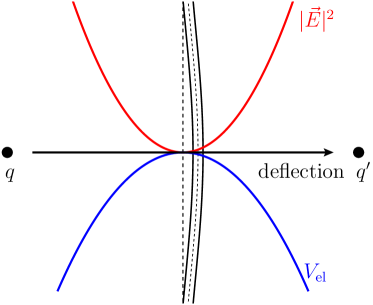
Figure 2: Resonator with electrodes modeled by point charges $q,q^{\prime}$. The field profile (red) leads to an inverted parabola for the dielectric potential (blue) around the equilibrium position.

One may also consider time dependent electric fields and it is convenient to separate between static and time dependent contributions,

$$F_{0} =F_{0}^{\mathrm{s}}+F_{0}(t)$$ (20)

$$W_{00} =W_{00}^{\mathrm{s}}+W_{00}(t)\,.$$ (21)

Whereas the time dependent contributions $F_{0}(t)$ and $W_{00}(t)$ generate drives applied to the nanobeam and will be considered in section VIII, we now focus on the constant contributions $F_{0}^{\mathrm{s}}$ and $W_{00}^{\mathrm{s}}$, which can be employed to tune the nanobeam.

The electrostatic force $F_{0}^{\mathrm{s}}$ causes a static deflection of the nanobeam and shifts its equilibrium position. However if the rod interacts with the photon fields of a nearby cavity, those fields will also cause a deflecting force. For convenience we choose $F_{0}^{\mathrm{s}}$ such that these two forces compensate and the equilibrium position remains unshifted (see section IV). The electrostatic potential associated to $W_{00}^{\mathrm{s}}$ in turn is an inverted harmonic potential that lowers the harmonic oscillation frequency of the nanobeam. Therefore, we consider

$$H_{\mathrm{m}}=\frac{\mathcal{P}^{2}}{2m^{*}}+\frac{1}{2}m^{*}\omega_{\mathrm{m}}^{2}\mathcal{X}^{2}+\frac{\beta}{4}\mathcal{X}^{4},$$ (22)

as the “tuned” mechanical Hamiltonian with a reduced frequency $\omega_{\mathrm{m}}^{2}\approx\omega_{\mathrm{m},0}^{2}-|W_{00}^{\mathrm{s}}|/m^{*}$. In a phononic description this Hamiltonian reads

$$H_{\mathrm{m}}=\hbar\omega_{\mathrm{m}}b^{{\dagger}}b+\hbar\frac{\lambda}{2}(b^{{\dagger}}+b)^{4}\,,$$ (23)

where the nonlinearity per phonon $\lambda=\zeta^{2}\lambda_{0}$ is now increased by a factor $\zeta^{2}=\left(\omega_{\mathrm{m},0}/\omega_{\mathrm{m}}\right)^{2}$, cf. Eq. (14). As an example, for maximum applied fields at the tube $E_{\parallel}\approx 1.2\times 10^{7}\,$Vm^-1 and $E_{\perp}\approx 1.8\times 10^{6}\,$Vm^-1 and a gap between the electrodes of size $D=40\,$nm (cf. Fig. 3), typical parameters discussed in Section V, yield $\zeta>3$ allowing to boost $\lambda$ by at least an order of magnitude.

For further calculations, it is convenient to express all observables in the energy eigenbasis of the Hamiltonian $H_{\mathrm{m}}$, so that

$$H_{\mathrm{m}}=\sum\limits_{n}E_{n}|n\rangle\langle n|\,,\qquad\mathcal{X}/x_{\mathrm{ZPM}}=\sum\limits_{nm}X_{nm}|n\rangle\langle m|\,,$$ (24)

where the energy eigenstates $\left\{|n\rangle\right\}$ and energy levels $E_{n}$, as well as the displacement matrix elements $X_{nm}$ have to be determined numerically. For small nonlinearites $\lambda\ll\omega_{\mathrm{m}}$ analytical expression can be obtained as the Hamiltonian (23) is approximately diagonal in Fock basis since one may apply a rotating wave approximation in the nonlinear part

$$H_{\mathrm{m}}\rightarrow H_{\mathrm{m}}^{\prime}=\hbar\omega_{\mathrm{m}}^{\prime}b^{{\dagger}}b+\hbar\frac{\lambda^{\prime}}{2}b^{{\dagger}}b^{{\dagger}}bb\,,$$ (25)

where $\omega_{\mathrm{m}}^{\prime}=\omega_{\mathrm{m}}+2\lambda^{\prime}$, $\lambda^{\prime}=6\lambda$ and the eigen-energies are given by $E_{n}\approx n\omega_{\mathrm{m}}^{\prime}+\frac{n(n-1)}{2}\lambda^{\prime}$.

The time dependent contributions $F_{0}(t)\mathcal{X}$ and $W_{00}(t)\mathcal{X}^{2}$ in turn can be used to drive or temporarily detune the resonator. This has been used in Rips2013 to perform local gate operations on nanobeams acting as qubits.

In the following section we will now discuss an optomechanical interaction between the nano resonator described by the Hamiltonian in equation (23) and the resonance modes of a high finesse cavity.

IV Optomechanical Model

We consider a typical optomechanical setup with a micro toroid cavity coupled to several nanomechanical resonators, where the displacement of the latter modifies the frequencies of the cavity modes. The cavity modes with frequencies $\omega_{i}$ that contribute to the dynamics are described by photon creation and annihilation operators ${a_{i}}^{{\dagger}}$ and ${a_{i}}$. They are each driven by a classical laser of input power $P_{i}$ and frequency $\omega_{\mathrm{L},i}$. The coupling strength between cavity mode $i$ and nanobeam $j$ is given by $G_{0,ij}x_{\mathrm{ZPM},j}$, where $G_{0,ij}=\tfrac{\partial\omega_{i}}{\partial\mathcal{X}_{j}}$ is the optical frequency shift per deflection $\mathcal{X}_{j}$. Thus, in a frame rotating with the laser field modes, the Hamiltonian describing the coupled system reads ($\hbar\rightarrow 1$)

$$H= \sum\limits_{i}\left[-\Delta_{i}{a_{i}}^{{\dagger}}a_{i}+\frac{\Omega_{i}}{2}\left(a_{i}^{{\dagger}}+a_{i}\right)\right]+\sum\limits_{j}H_{\mathrm{m},j}$$

$$+\sum\limits_{ij}G_{0,ij}{a_{i}}^{{\dagger}}a_{i}\mathcal{X}_{j}\,.$$ (26)

Here we have introduced the laser detunings denoted by $\Delta_{i}=\omega_{\mathrm{L},i}-\omega_{i}$ and drive amplitudes $\Omega_{i}/2=\sqrt{P_{i}\kappa_{\mathrm{ex},i}/\hbar\omega_{\mathrm{L},i}}$, with $\kappa_{\mathrm{ex},i}$ being the cavity decay rates into the associated outgoing electromagnetic modes.

Both the field inside the cavity and the mechanical motion are subject to damping, which in the regime of weak optomechanical coupling, small nonlinearity and low mechanical occupation is well described by a master equation with Lindblad form damping terms. With the decay rates for the cavity modes $\kappa_{i}$ and the mechanical damping rates $\gamma_{j}$, this master equation reads

$$\dot{\rho}=-\mathrm{i}\left[H,\rho\right] +\sum\limits_{i}\frac{\kappa_{i}}{2}\mathcal{D}(a_{i})\rho\,+$$ (27)

$$+\sum\limits_{j}\frac{\gamma_{j}}{2}\left[(\overline{n}_{j}+1)\mathcal{D}(b_{j})\rho+\overline{n}_{j}\mathcal{D}(b^{{\dagger}}_{j})\rho\right]\,.$$

Here we introduced the Lindblad form dissipator $\mathcal{D}(\hat{o})\rho=2\hat{o}\rho\hat{o}^{{\dagger}}-\hat{o}^{{\dagger}}\hat{o}\rho-\rho\hat{o}^{{\dagger}}\hat{o}$, as well as the Bose occupation number $\overline{n}_{j}=\left[\exp\left(\frac{\hbar\omega_{\text{m},j}}{k_{\mathrm{B}}T}\right)-1\right]^{-1}$ of the phonon bath mode with frequency $\omega_{\text{m},j}$ at temperature $T$. A more precise treatment of the mechanical damping accounts for the fact that, due to the mechanical nonlinearity, there is more than one bath mode resonantly coupling to the mechanical mode. However, for small nonlinearity, equation (27) proofs to be sufficiently accurate.

As usual, we expand the cavity field operators around their steady state values and adopt a shifted representation $a_{i}\rightarrow a_{i}+\alpha_{i}$, with $\alpha_{i}=\Omega_{i}/(2\Delta_{i}+\mathrm{i}\kappa_{i})$, in which the master equation has the same form as in equation (27) but with the shifted system Hamiltonian

$$H^{\prime}= -\sum\limits_{i}\Delta_{i}{a_{i}}^{{\dagger}}a_{i}+\sum\limits_{j}H_{\mathrm{m},j}$$

$$+\sum\limits_{ij}\left(\frac{g_{\mathrm{m},ij}^{*}}{2}a_{i}+\text{H.c.}\right)\left(b^{{\dagger}}_{j}+b_{j}\right)$$ (28)

with $g_{\mathrm{m},ij}=2\alpha_{i}G_{0,ij}x_{\mathrm{ZPM},j}$ and where we have dropped the nonlinear terms $\propto{a_{i}}^{{\dagger}}a_{i}(b^{{\dagger}}_{j}+b_{j})$ in the coupling, which is valid for $\left\langle{a_{i}}^{{\dagger}}a_{i}\right\rangle\ll|\alpha_{i}|^{2}$. We have also assumed that the static electric fields for each beam are chosen such that $F_{0,j}^{\mathrm{s}}=-\hbar\sum_{i}G_{0,i}|\alpha_{i}|^{2}$, so that their equilibrium positions are undeflected.

We now turn to discuss a possible experimental setup that would allow to explore the physics described by the model presented in equation (27).

V Setup

     

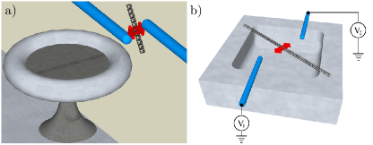
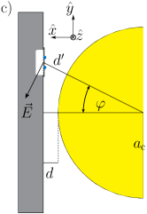
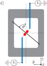
Figure 3: a) Microtoroid cavity with nearby CNT (not to scale). b) NEMS-chip with CNT-resonator and electrodes. c) Schematic top view of the NEMS chips with the CNT oscillating in the $\hat{z}$-$\hat{y}$-plane. d) Schematic cross-sectional view of the NEMS-Chip and the cavity rim (yellow). The NEMS-chip is mounted in the evanescent cavity field at a distance $d$ to the cavity rim surface. The nanoresonator is displaced from the closest point to allow for an optomechanical coupling that is linear in the resonator’s deflection.

For the experimental realization of the model in equation (27), we envisage a setup as shown in Fig. 3, comprising a NEMS chip containing the nanobeam resonators and a high finesse toroidal microcavity nphys1425 ; PhysRevLett.103.053901 ; Lee10 . Each nanobeam resonator consists of a suspended single-walled carbon nanotube (CNT) with radius $R$ ($c_{\mathrm{s}}=2.1\times 10^{4}\,$ms^-1, $\mu=(2\pi R)\times 7.6\times 10^{-7}\,$kgm^-2) science.1176076 ; science.1174290 , and has electrodes in its vicinity that generate the electric fields for controlling and driving it. Furthermore, the nanoresonator interacts with the evanescent field of the microcavity via optical gradient forces (see section VI). Given the state of the art, a CNT is a favorable system to implement the proposed optoelectromechanical scheme Hofmann13 ; Waissman13 ; Stapfner13 . In particular, the intrinsic nonlinearity per phonon scales as $\lambda_{0}\propto\left(\tilde{\kappa}^{2}m\right)^{-1}$, which favors small transverse dimensions and masses. Additionally, carbon nanotubes show ultra-low dissipation doi:10.1021/nl900612h , that is expected to decrease further in the regime of small amplitudes nnano.2011.71 . It is convenient to use ($10$,$0$) CNTs with radius $R=$0.39\text{\,}\mathrm{nm}$$, as these tubes show relatively large static polarizabilities with $\alpha_{||}=143\left(4\pi\epsilon_{0}\text{\AA{}}{}^{2}\right)$, $\alpha_{\perp}=10.9\left(4\pi\epsilon_{0}\text{\AA{}}{}^{2}\right)$ PhysRevLett.96.166801 , where $\alpha_{||}$ ($\alpha_{\perp}$) is the polarizability parallel (perpendicular) to the tube axis. To obtain nonlinearities that are large enough, it is convenient to use CNT lengths below $1\text{\,}\mathrm{\SIUnitSymbolMicro m}$ —for $L=$1\text{\,}\mathrm{\SIUnitSymbolMicro m}$$ we have $\omega_{\mathrm{m},0}=$20.6\text{\,}\mathrm{MHz}$$ and $\lambda_{0}=$2.24\text{\,}\mathrm{kHz}$$.

The cavity is a silica ($n_{\mathrm{c}}=1.44$) microtoroid with resonant wavelengths $2\pi c/\omega_{j}\approx\lambda_{c}=$1.1\text{\,}\mathrm{\SIUnitSymbolMicro m}$$, circumference $L_{\mathrm{c}}\sim$1\text{\,}\mathrm{mm}$$, finesse $\mathcal{F}_{\mathrm{c}}=3\times 10^{6}$ kippenberg:6113 and mode volume $V_{\mathrm{c}}\approx L_{\mathrm{c}}\times$6\text{\,}{\mathrm{\SIUnitSymbolMicro m}}^{2}$$. These parameters correspond to $a_{c}\approx$2.0\text{\,}\mathrm{\SIUnitSymbolMicro m}$$, $\xi\approx 0.2$ and a decay length of the evanescent field $\kappa_{\perp}^{-1}\approx$0.17\text{\,}\mathrm{\SIUnitSymbolMicro m}$$ [cf. Eq. (41) in Section VI]. The NEMS chip is placed at a distance $d=$50\text{\,}\mathrm{nm}$$ from the cavity rim. The CNT-resonator is displaced from the closest point to allow for a linear coupling, as the resonator moves in the plane of the chip’s surface (cf. Section VI), and the electrodes are aligned parallel to the rim of the cavity to minimize additional cavity losses they might induce, see section VII.

In the following two sections we analyze important practical aspects of the envisioned implementation with a carbon nanotube coupled to a toroidal microcavity in more detail. Thus, readers who are only interested in the results of the discussed mechanism may directly turn to section VIII.

VI Optomechanical coupling

In this section we derive an estimate for the coupling between the mechanical displacement and the cavity field. The coupling arises as the energy of the dielectric oscillator in the evanescent electric field depends on the field strength at the location of the oscillator. As the evanescent field decays with distance to the cavity rim, altering the oscillator-cavity distance by displacing the oscillator results in a change of energy. Thus, the coupling part of the Hamiltonian is given by

$$H_{\mathrm{c}}=-\frac{1}{2}\int_{V_{R}}\vec{P}(\vec{r})\cdot\vec{E}(\vec{r}){\rm d}V$$ (29)

where the polarization is $\vec{P}(\vec{r})=\overleftrightarrow{\alpha}\cdot\vec{E}(\vec{r})$ with $\overleftrightarrow{\bf\alpha}$ the screened polarizability tensor and $\vec{E}$ the cavity field. The integration is taken over the oscillator volume $V_{R}$ and without loss of generality we consider a single cavity mode with resonant frequency $\omega_{\mathrm{c}}$.

Given the dimensions of the toroidal microcavity, its torus can be locally modeled as a cylindrical waveguide of radius $a_{\mathrm{c}}$ —note that this differs from the definition of $a_{\mathrm{c}}$ used in Ref. Rips2012, by a factor of $1.44$ [cf. below Eq. (40)]. We introduce cylindrical coordinates $(r,\phi,z)$ with the $\hat{z}$-direction along the waveguide axis (cf. Fig. 3c) and consider TE_0,1 modes, as a transverse electric field is advantageous to suppress loss mechanisms that are discussed in section VII. The corresponding transverse fields are given by Jackson8

$$B_{r}= \mathrm{i}\frac{k_{||}}{\gamma^{2}}\frac{\partial B_{z}}{\partial r}\,,$$

$$E_{\varphi}= -\frac{\omega_{\mathrm{c}}}{k_{||}}B_{r}\,,$$ (30)

for the field inside the waveguide, $r<a_{\mathrm{c}}$, and

$$B_{r}= -\mathrm{i}\frac{k_{||}}{\kappa_{\bot}^{2}}\frac{\partial B_{z}}{\partial r}\,,$$ (31)

$$E_{\varphi}= -\frac{\omega_{\mathrm{c}}}{k_{||}}B_{r}\,,$$ (32)

outside the waveguide, $r>a_{\mathrm{c}}$. The axial field reads

$$B_{z}(r,z) =B_{z}(0)J_{0}(\gamma r)\mathrm{e}^{\mathrm{i}k_{||}z}\,, r<a_{\mathrm{c}}\,,$$ (33)

$$B_{z}(r,z) =\tilde{\xi}B_{z}(0)\frac{K_{0}^{(1)}(\kappa_{\bot}r)}{K_{0}^{(1)}(\kappa_{\bot}a_{\mathrm{c}})}\mathrm{e}^{\mathrm{i}k_{||}z}\,, r>a_{\mathrm{c}}\,,$$ (34)

with the modified Bessel function $K_{0}^{(1)}$ and the Bessel function of the first kind $J_{0}$. Here $\tilde{\xi}=B_{z}(a_{\mathrm{c}},z)/B_{z}(0,z)$, $k_{||}$ is the wavevector component parallel to the waveguide axis and $\mathrm{i}\kappa_{\bot}$ and $\gamma$ are the transverse wave vectors outside and inside the waveguide, respectively. Henceforth, we assume a refractive index such that $n_{\mathrm{c}}^{2}-1\sim n_{\mathrm{c}}^{2}$ and a frequency $\omega_{\mathrm{c}}$ well above cutoff, i.e. $(n_{\mathrm{c}}ka_{\mathrm{c}}/x_{1,1})^{2}\gg 1$ —where $k=\omega_{\mathrm{c}}/c$ and $x_{1,1}\approx 3.8$ is the first zero of $J_{1}(x)$. These assumptions imply that $k_{||}\approx n_{\mathrm{c}}k$, $\kappa_{\perp}\approx\sqrt{n_{\mathrm{c}}^{2}-1}k$, $\gamma\ll\kappa_{\perp}$, $\kappa_{\perp}a_{\mathrm{c}}\gg 1$, and $a_{\mathrm{c}}\gamma\approx x_{1,1}$. Within these approximations, the ratio of the axial magnetic field at $r=a_{\mathrm{c}}$ to its value at the origin is given by $\tilde{\xi}=J_{0}(x_{1,1})\approx-0.4$, and the evanescent field can be written as

$$E_{\varphi}(r)\approx-\mathrm{i}\frac{\omega_{\mathrm{c}}}{\kappa_{\bot}}\tilde{\xi}B_{z}(0)\sqrt{\frac{a_{\mathrm{c}}}{r}}\mathrm{e}^{-\kappa_{\bot}(r-a_{\mathrm{c}})}\mathrm{e}^{\mathrm{i}nkz}\,.$$ (35)

This field will later be used to estimate losses induced by the electrodes. In order to determine the optomechanical coupling strength, we write the electric field in its quantized form

$$\vec{E}(\vec{r})=\sqrt{\frac{\hbar\omega_{\mathrm{c}}}{2\epsilon_{0}}}(a^{{\dagger}}+a)u_{\varphi}(\vec{r})\hat{\varphi}\,,$$ (36)

with photon creation (annihilation) operators $a^{{\dagger}}(a)$ and where $\vec{u}(\vec{r})\propto\vec{E}(\vec{r})$ is the corresponding normalized eigenmode, satisfying

$$\int\frac{\epsilon(\vec{r})}{\epsilon_{0}}\left|\vec{u}(\vec{r})\right|^{2}{\rm d}V=1\,.$$ (37)

We consider the following definition for the mode volume

$$V_{\mathrm{c}}=\int{\rm d}V\frac{\epsilon(\vec{r})|\vec{E}(\vec{r})|^{2}}{n_{\mathrm{c}}^{2}\epsilon_{0}|\vec{E}_{\mathrm{max}}|^{2}}\,,$$ (38)

From Eqs. (30) and (33) and properties of the Bessel functions, we obtain that the maximum electric field inside the cavity is given by

$$|\vec{E}_{\mathrm{max}}|=\frac{\omega_{\mathrm{c}}}{\gamma}\left|B_{z}(0)\right|J_{1}\left(x_{*}\right)\approx\frac{\omega_{\mathrm{c}}}{\gamma}\frac{\left|B_{z}(0)\right|}{1.7}\,,$$ (39)

where $x_{*}$ is the first positive root of $J_{0}(x)=J_{2}(x)$. Thus, neglecting the small contributions of the evanescent part to the integrations in Eqs. (37) and (38) which are higher order in $1/\kappa_{\perp}a_{\mathrm{c}}$, we obtain from Eqs. (35)-(39)

$$u_{\varphi}(\vec{r})\approx\frac{-\xi}{n_{\mathrm{c}}\sqrt{V_{\mathrm{c}}}}\sqrt{\frac{a_{\mathrm{c}}}{r}}\,\mathrm{e}^{-\kappa_{\bot}(r-a_{\mathrm{c}})}\,$$ (40)

for $r>a_{\mathrm{c}}$. Here, $V_{\mathrm{c}}\approx 0.5\,\pi a_{\mathrm{c}}^{2}L_{\mathrm{c}}$ and

$$\xi=\frac{\gamma|\tilde{\xi}|}{\kappa_{\perp}J_{1}(x_{*})}=\frac{\lambda_{\mathrm{c}}x_{1,1}\left|J_{0}(x_{1,1})\right|}{2\pi a_{\mathrm{c}}\sqrt{n_{\mathrm{c}}^{2}-1}J_{1}(x_{*})}\approx\frac{0.42\,\lambda_{\mathrm{c}}}{a_{\mathrm{c}}\sqrt{n_{\mathrm{c}}^{2}-1}}$$ (41)

denotes the ratio of the electric field at the waveguide’s surface to the maximum field $E_{\mathrm{max}}$.

The zero point motion $x_{\mathrm{ZPM}}$ of the oscillator is small compared to the decay length $1/\kappa_{\bot}$ of the evanescent field and the same holds for the transverse dimensions of the oscillator. Thus, we can linearize $\vec{E}(\vec{r})\cdot\overleftrightarrow{\alpha}\cdot\vec{E}(\vec{r})$ around the equilibrium position of the nanoresonator and assume that the electric field is constant everywhere inside the resonator volume $V_{R}$. Subsequently, by comparing the Hamiltonians (29) and (26), and using Eqs. (36) and (40), we find for the opto-mechanical coupling rate,

$$G_{0}\approx\frac{\omega_{\mathrm{c}}\alpha_{||}\kappa_{\bot}L\xi^{2}}{n_{\mathrm{c}}^{2}\epsilon_{0}V_{\mathrm{c}}}\mathrm{e}^{-2\kappa_{\bot}d}C_{\mathrm{corr}}\,.$$ (42)

Here, we have neglected the contribution of the perpendicular polarizability since, for carbon nanotubes, the perpendicular polarizability is typically one order of magnitude smaller than the parallel one, and again used $\kappa_{\perp}a_{\mathrm{c}}\gg 1$ so that only the derivative of the exponential factor is relevant. The geometry of the setup we consider here is illustrated in figure 3 and the dependence on the alignment and positioning of the nanotube is accounted for in the correction factor $C_{\mathrm{corr}}$. For a TE_0,1 mode of the cavity field, the electric field is directed along $\hat{\varphi}$, i.e. tangential to the cavity rim, while the nanotube is aligned along $\vec{e}_{\mathrm{nt}}=\cos\theta^{\prime}\hat{z}+\sin\theta^{\prime}\hat{y}$. In addition, the deflection of the nanotube in the direction $\vec{e}_{\mathrm{osc}}=\cos\theta^{\prime}\hat{y}-\sin\theta^{\prime}\hat{z}$ is not aligned with the interaction-energy gradient, which is approximately along $\hat{r}=\cos\varphi\hat{x}+\sin\varphi\hat{y}$. Finally, if $d$ is the distance of the chip to the cavity rim, the actual distance of the oscillator to the rim is $d^{\prime}=(a_{\mathrm{c}}+d)/\cos\varphi-a_{\mathrm{c}}$. Taking into account these various issues, we find for the correction factor

$$C_{\mathrm{corr}}\approx\mathrm{e}^{-2\kappa_{\bot}(d+a_{\mathrm{c}})(\text{sec}\varphi-1)}\sin^{2}\theta^{\prime}\cos\theta^{\prime}\cos^{2}\varphi\sin\varphi\,.$$ (43)

This is maximized for $\sin^{2}\theta^{\prime}_{*}=2/3$ and $\varphi_{*}\approx 1/\sqrt{2\kappa_{\bot}(d+a_{\mathrm{c}})}$, where we consider the leading order in the small parameter $1/2\kappa_{\perp}(d+a_{\mathrm{c}})$. These optimal angles yield $C_{\mathrm{corr}}\approx 0.17/\sqrt{\kappa_{\bot}(d+a_{\mathrm{c}})}$, resulting in $1/C_{\mathrm{corr}}\approx 22$ for the parameters introduced in Section V (i.e. $n_{\mathrm{c}}=1.44$ and $d\ll a_{\mathrm{c}}\approx$2.0\text{\,}\mathrm{\SIUnitSymbolMicro m}$$). Finally, for those typical values we obtain $G_{0}\approx 1.02\times 10^{10}\mathrm{Hz}/\mathrm{m}$.

VII Loss Mechanisms

In addition to the well known loss mechanisms of photon losses from the cavity and intrinsic phonon losses of the mechanical resonator Wilson-Rae08 ; Remus09 , there can be further sources of loss in our setup due to the presence of the tip electrodes. In this section we show that these additional loss mechanisms are negligible for the parameters we envision.

VII.1 Cavity losses induced by metallic nanotube electrodes

Exploiting the nonlinearity of the nanoresonators to control their dynamics demands a high-$Q$ optical cavity as the linewidth $\kappa$ needs to be at most comparable to the mechanical nonlinearity $\lambda$. Using conventional metallic electrodes to generate the inhomogeneous control fields can potentially increase the cavity losses. To achieve the necessary low losses it is crucial to have deep subwavelength transverse dimensions for the electrodes.

We now give an estimate of the photon losses that may be induced by such electrodes and show that these are negligible. To do so, we model the electrodes as metallic cylinders and assume that their radius $R^{\prime}$ is much smaller than the decay length of the evanescent cavity field, $R^{\prime}\ll\kappa_{\bot}^{-1}$. We assume the electrodes to be parallel to the waveguide representing the cavity rim, with a small misalignment angle $\theta$. For the relevant TE_0,n modes, the losses result solely from the misalignment, as in the small radius regime considered they arise only from the field along the electrode axis which vanishes for $\theta=0$. The resulting finesse $\mathcal{F}$ for the cavity can be obtained from the finesses $\mathcal{F}_{i}$ associated to different decay channels, which can be assumed to be independent such that

$$\frac{1}{\mathcal{F}}=\sum_{i}{\frac{1}{\mathcal{F}_{i}}}\,.$$ (44)

For each loss channel, the finesse $\mathcal{F}_{i}$ can be determined from the ratio of the power circulating in the cavity $P_{c}$ to the fraction of power that it lost through the respective channel $P_{i}$, using that the time-averaged stored energy and free spectral range are given, respectively, by $\langle U\rangle=P_{c}(n_{\mathrm{c}}L_{\mathrm{c}}/c)$ and $\Delta\omega=2\pi c/n_{\mathrm{c}}L_{\mathrm{c}}$. Thus, we arrive at

$$\frac{1}{\mathcal{F}_{i}}=\frac{P_{i}}{\Delta\omega\langle U\rangle}=\frac{P_{i}}{2\pi P_{c}}\,.$$ (45)

The loss channels that will be considered subsequently are (1) scattering by the “bulk” of the electrodes modeled as a single metallic cylinder , (2) scattering by the “gap” between the electrodes and (3) absorption. The independence between the contributions (1) and (2) assumed in Eq. (44) amounts to neglecting the interference between them which is permissible when estimating an upper bound.

Incident field and circulating power

For our calculations, we introduce new cylindrical co-ordinates $(r^{\prime},\varphi^{\prime},z^{\prime})$ for the electrode with the $z^{\prime}$-direction along its axis. We first express the cavity field that is incident on the electrode in these primed coordinates. The result will later be used to determine the scattered and absorbed fractions of the incident power.

To this end, we consider the projection of the electric field determined in Section VI onto the electrode’s axis, see Fig. 4,

$$E_{z^{\prime}}^{(\mathrm{in})}(z^{\prime})=\left.\hat{z}^{\prime}\cdot\hat{\varphi}\,\,E_{\varphi}\right|_{r^{\prime}=0}\,,$$ (46)

which completely determines the losses in the small radius regime considered. The origin of the primed axis lies at $(d+a_{\mathrm{c}},0,0)$ and the relevant unit vectors are given by

$$\hat{z}^{\prime} = \sin\theta\hat{y}+\cos\theta\hat{z}$$ (47)

$$\hat{\varphi} = -\sin\varphi\hat{x}+\cos\varphi\hat{y}\,.$$ (48)

For points on the $z^{\prime}$-axis we have

$$\cos\varphi = \frac{d+a_{\mathrm{c}}}{r}\,,$$ (49)

$$r = \sqrt{(d+a_{\mathrm{c}})^{2}+z^{\prime 2}\sin^{2}\theta}\,,$$ (50)

$$z = z^{\prime}\cos\theta\,.$$ (51)

For our further calculations it is convenient to express the incident field via its Fourier transform $E_{z^{\prime}}^{(\mathrm{in})}(k^{\prime})=\int_{-\infty}^{\infty}E_{z^{\prime}}^{(\mathrm{in})}(z^{\prime})\mathrm{e}^{-\mathrm{i}k^{\prime}z^{\prime}}{\rm d}z^{\prime}$. Using this and equations (47)-(51) in equations (35) and (46) we arrive at

$$E_{z^{\prime}}^{(\mathrm{in})}(\tilde{k})= \frac{-\mathrm{i}\omega_{\mathrm{c}}}{\kappa_{\bot}}s\sqrt{a_{\mathrm{c}}(d+a_{\mathrm{c}})}\tilde{\xi}\mathrm{e}^{-\kappa_{\bot}d}B_{z}(0)\,\times$$

$$\times\underbrace{\int\limits_{-\infty}^{\infty}{\rm d}x\frac{\mathrm{e}^{-\kappa_{\bot}(d+a_{\mathrm{c}})(\sqrt{1+x^{2}}-1+\mathrm{i}\tilde{k}x)}}{(1+x^{2})^{3/4}}}_{F}\,,$$ (52)

where we have substituted $x=z^{\prime}\sin\theta/(d+a_{\mathrm{c}})$ and $\tilde{k}=(k^{\prime}-n_{\mathrm{c}}k\cos\theta)/(\kappa_{\bot}\sin\theta)$. One can find an approximation for the integral $F$ by applying the method of steepest descents, using $\kappa_{\bot}(d+a_{\mathrm{c}})\gg 1$ and $d\sim\kappa_{\bot}^{-1}\ll a_{\mathrm{c}}$, which for $|\theta|\ll 1$ yields

$$|F|\approx\sqrt{\frac{2\pi}{(d+a_{\mathrm{c}})\kappa_{\bot}}}\mathrm{e}^{-\kappa_{\bot}(d+a_{\mathrm{c}})|\tilde{k}|}$$ (53)

Figure 4: Relative alignment of electrode coordinates $(r^{\prime},\varphi^{\prime},z^{\prime})$ and waveguide coordinates $(r,\varphi,z)$. The misalignment is determined by a small angle $\theta$.

Finally, we determine the circulating power to leading order in $1/\kappa_{\perp}a_{\mathrm{c}}$, which is given by

$$P_{c} =\int{\rm d}A\cdot\langle\vec{S}\rangle=\,\frac{\pi n_{\mathrm{c}}c}{\text{\textmu}_{0}}\left(\frac{k}{\gamma}\right)^{2}\left|B_{z}(0)\right|^{2}\int\limits_{0}^{a_{\mathrm{c}}}rJ_{1}^{2}(\gamma r){\rm d}r$$

$$=\frac{\pi}{2}J_{2}^{2}(x_{1,1})\frac{cn_{\mathrm{c}}}{\text{\textmu}_{0}}\left(\frac{ka_{\mathrm{c}}}{\gamma}\right)^{2}\left|B_{z}(0)\right|^{2}$$

$$\approx 0.25\frac{cn_{\mathrm{c}}}{\text{\textmu}_{0}}\left(\frac{ka_{\mathrm{c}}}{\gamma}\right)^{2}\left|B_{z}(0)\right|^{2},$$ (54)

where we have used Eqs. (30) and (33), that $\pi\int\limits_{0}^{1}xJ_{1}^{2}(x_{1,1}x){\rm d}x=\frac{\pi}{2}J_{2}^{2}(x_{1,1})$, and the time-averaged Poynting vector $\langle\hat{z}\cdot\vec{S}\rangle=\frac{1}{2}\Re\{E_{\varphi}^{*}B_{r}\}/\text{\textmu}_{0}$ with the vacuum permeability µ₀.

Scattering losses

Here, we model the electrodes as a single metallic cylinder which for simplicity is assumed to be perfectly conducting since this maximizes the scattering and, thus, provides an estimate of an upper bound to the corresponding losses that is independent of material properties —naturally for the transparent electrode scenario considered below, in Section VII.1.d, these losses would be substantially smaller than this upper bound. We expand the scattered field into solutions of the wave equation in cylindrical coordinates for the electrode. As the radius of the electrode $R^{\prime}$ is much smaller than the wavelength of the incident field $\lambda_{\mathrm{c}}$, all contributions to the scattered power are suppressed at least like $(kR^{\prime})^{4}$, except for s-wave scattering of TM modes, for which the suppression is only logarithmic. This can be understood in terms of the Taylor expansions of the corresponding cylindrical harmonics and the incident field. In turn, to determine the TM s-wave scattering to leading order in $kR^{\prime}$, the incident field can be assumed to be constant for a given cross section and determined by the field at the electrode’s center $E_{z^{\prime}}^{(\mathrm{in})}(z^{\prime})$. We neglect multiple scattering between the waveguide and the electrode and ignore the dielectric substrate of the latter. Thus, the scattered field $E_{z^{\prime}}^{(s)}$ is determined from the homogeneous boundary condition at the surface of the electrode $E_{z^{\prime}}|_{r^{\prime}=R^{\prime}}=(E_{z^{\prime}}^{(\mathrm{in})}+E_{z^{\prime}}^{(s)}+E_{z^{\prime}}^{(e)})|_{r^{\prime}=R^{\prime}}=0$, and an outgoing-wave boundary condition at infinity for $E_{z^{\prime}}^{(s)}$ —here $E_{z^{\prime}}^{(e)}$ is the evanescent contribution.

The transverse fields of an outgoing TM solution with $z^{\prime}$-dependence $\exp\left(\mathrm{i}k^{\prime}z^{\prime}\right)$ are given by

$$\vec{E}_{\bot}^{(s)} = \mathrm{i}\frac{k^{\prime}}{k^{2}-k^{\prime 2}}\nabla_{\bot}E_{z^{\prime}}^{(s)}\,,$$ (55)

$$\vec{H}_{\bot}^{(s)} = c\epsilon_{0}\frac{k}{k^{\prime}}\hat{z}^{\prime}\times\vec{E}_{\bot}^{(s)}\,,$$ (56)

with $k^{\prime 2}<k^{2}$. For $k^{\prime 2}>k^{2}$ the solution is evanescent and does not contribute to the scattered power. For s-wave scattering $E_{z^{\prime}}^{(s)}(k^{\prime})\propto H_{0}^{(1)}(k_{\bot}r^{\prime})\mathrm{e}^{\mathrm{i}k^{\prime}z^{\prime}}$, where $k_{\bot}^{2}=k^{2}-k^{\prime 2}$, and to leading order in $kR^{\prime}$, the scattered field can be written as

$$E_{z^{\prime}}^{(s)}(r^{\prime},\varphi^{\prime},z^{\prime})\approx-\int\limits_{-k}^{k}\frac{{\rm d}k^{\prime}}{2\pi}E_{z^{\prime}}^{(\mathrm{in})}(k^{\prime})\frac{H_{0}^{(1)}(\sqrt{k^{2}\!-\!k^{\prime 2}}r^{\prime})}{\mathrm{i}\frac{2}{\pi}\ln\left(\sqrt{k^{2}\!-\!k^{\prime 2}}R^{\prime}\right)}\mathrm{e}^{ik^{\prime}z^{\prime}}\,,$$ (57)

where $E_{z^{\prime}}^{(\mathrm{in})}(k^{\prime})$ is the Fourier transform of the incident field $E_{z^{\prime}}^{(\mathrm{in})}(z^{\prime})$ and we have used the approximation $H_{0}^{(1)}(x)\approx\mathrm{i}(2/\pi)\ln x$ for $|x|\ll 1$. We calculate the scattered power by integrating the energy flux across a cylinder coaxial with the electrode with radius $R_{*}\rightarrow\infty$. Thus, from Eqs. (55)-(57) we obtain for the scattered power

$$P_{\mathrm{s}}\approx \,\frac{\pi}{4}c\epsilon_{0}\int\limits_{-k}^{k}{\rm d}k^{\prime}\frac{k\left|E_{z^{\prime}}^{(\mathrm{in})}(k^{\prime})\right|^{2}}{(k^{2}-k^{\prime 2})\ln^{2}(\sqrt{k^{2}-k^{\prime 2}}R^{\prime})}$$

$$< \,\pi c\epsilon_{0}\text{max}\left.\left\{\left|E_{z^{\prime}}^{(\mathrm{in})}(k^{\prime})\right|^{2}\right\}\right|_{|k^{\prime}|\leq k}$$

$$\times\underbrace{2\int\limits_{0}^{k}{\rm d}k^{\prime}\frac{k}{(k^{2}-k^{\prime 2})\ln^{2}\left[(k^{2}-k^{\prime 2}){R^{\prime}}^{2}\right]}}_{G}$$ (58)

where we have used

$$\langle\hat{r}^{\prime}\cdot\vec{S}\rangle=\frac{1}{2}\Re\{\hat{r}^{\prime}\cdot({\vec{E}}^{*}\times\vec{H})\}=\frac{1}{2}\Re\left\{\frac{\mathrm{i}c\epsilon_{0}k}{k^{\prime 2}-k^{2}}\frac{\partial E_{z^{\prime}}^{(s)}}{\partial r^{\prime}}{E_{z^{\prime}}^{(s)}}^{*}\right\}$$

and $H_{0}^{(1)}(x)\approx\sqrt{2/\pi x}\exp\left[\mathrm{i}(x-\pi/4)\right]$ for $|x|\gg 1$. The integral $G$ can be estimated by performing the substitution $v=\ln[(k-k^{\prime})/2k]/\ln(2kR)$ and considering $kR\ll 1$, which yields $G\approx 1/(2|\ln(2kR^{\prime})|)$.

Hence, from Eqs. (45), (52)-(54), (58) and (41), and using $\sin\theta\approx\theta$ and $\cos\theta\approx 1$ for $|\theta|\ll 1$, and $\kappa_{\perp}\approx\sqrt{n_{\mathrm{c}}^{2}-1}k$ we arrive at

$$\frac{1}{\mathcal{F}_{s}}<\frac{\mathrm{e}^{-2k\left[d\sqrt{n_{\mathrm{c}}^{2}-1}+(d+a_{\mathrm{c}})\frac{n_{\mathrm{c}}-1}{|\theta|}\right]}}{n_{\mathrm{c}}\left(ka_{\mathrm{c}}\sqrt{n_{\mathrm{c}}^{2}-1}\right)^{3}|\ln 2kR^{\prime}|}\,.$$ (59)

If we now use that for relevant parameters $d\ll a_{\mathrm{c}}$, $a_{\mathrm{c}}>\lambda_{\mathrm{c}}$ and $|\theta|<\sqrt{\frac{n_{\mathrm{c}}-1}{n_{\mathrm{c}}+1}}$, we find a lower bound for the finesse associated to scattering losses,

$$\mathcal{F}_{\mathrm{s}}>16\,n_{\mathrm{c}}\left(n_{\mathrm{c}}^{2}-1\right)^{3/2}\ln\left(\frac{\lambda_{\mathrm{c}}}{4\pi R^{\prime}}\right)\mathrm{e}^{4\pi\frac{n_{\mathrm{c}}-1}{|\theta|}}\,,$$ (60)

which is independent of the ratio $a_{\mathrm{c}}/\lambda_{\mathrm{c}}$. Thus, for $\lambda=$1.1\text{\,}\mathrm{\SIUnitSymbolMicro m}$$, $R^{\prime}\leq$10\text{\,}\mathrm{nm}$$, $n_{\mathrm{c}}=1.44$ and $\theta\leq$10\text{\,}\mathrm{\SIUnitSymbolDegree}$$, we find $\mathcal{F}_{\mathrm{s}}>3\times 10^{15}$. Hence losses due to scattering are clearly sufficiently suppressed for electrodes of subwavelength radius that are approximately aligned with the cavity rim.

Gap contribution to scattering losses

So far we have considered scattering from one single continuous electrode. Actually, our setup comprises two electrodes, see figure 3, separated by a gap in which the nanomechanical oscillator is positioned. We now estimate an upper bound to the additional losses that this gap may induce. Here we assume as before $\theta\ll 1$ so that the gap is much smaller than the distance over which substantial currents are induced in the electrodes and one may consider $\theta=0$ for this estimate. Denoting the direction joining the electrodes by $\hat{z}"$, we focus on the relevant regime $D\gg 2R^{\prime}$ so that one can assume that only the incident field component along $\hat{z}"$ is screened by them. We model the gap of size $D$ as a perfectly conducting sphere with radius $D/2$ subject to an external field along $\hat{z}"$ determined by ${\vec{E}}^{(\mathrm{in})}\cdot\hat{z}"=E_{\varphi}^{(\mathrm{in})}\cos\theta^{\prime}\cos\varphi^{\prime}$. This should provide an upper bound for the magnitude of the total induced dipole $p$, which in turn determines the leading contribution in $kD$ to the scattered power. Thus we find $p\sim\frac{\pi}{2}\epsilon_{0}D^{3}|E_{\varphi}^{(\mathrm{in})}|\cos\theta^{\prime}_{*}\cos\varphi^{\prime}_{*}$ Jackson8 for optimal placement, which yields for the scattered power

$$P_{\mathrm{g}}\lesssim\frac{\pi}{48}\epsilon_{0}ck^{4}D^{6}\left[\frac{\omega_{\mathrm{c}}\xi}{\gamma}\left|B_{z}(0)\right|J_{1}(x_{*})\right]^{2}\mathrm{e}^{-2\kappa_{\bot}d}\cos^{2}\theta^{\prime}_{*}\,.$$ (61)

Here we have used Eq. (35), $d^{\prime}\ll a_{\mathrm{c}}$ and $\cos\varphi^{\prime}_{*}\approx 1$. Along the same lines as before, using Eqs. (54) and (45) and $\sin^{2}\theta^{\prime}_{*}=2/3$, the associated finesse reads

$$\mathcal{F}_{\mathrm{g}}\gtrsim 0.8\,\frac{n_{\mathrm{c}}a_{\mathrm{c}}^{4}\lambda_{\mathrm{c}}^{2}}{D^{6}\xi^{2}}\left(n_{\mathrm{c}}^{2}-1\right)\mathrm{e}^{\frac{4\pi d}{\lambda_{\mathrm{c}}}\sqrt{n_{\mathrm{c}}^{2}-1}}$$ (62)

which yields $\mathcal{F}_{g}\gtrsim 3\times 10^{9}$ for the parameters discussed in Section V and $D=40\,$nm. Thus, additional scattering losses due to the gap between the electrodes are also negligible.

Absorption losses

We assume here transparent electrodes afforded by cylindrical shells with 2D conductivity $\sigma$ that absorb the power

$$P_{\mathrm{a}}=\frac{1}{2}\int\limits_{-\infty}^{\infty}{\rm d}z^{\prime}\Re\left\{I^{*}E_{z^{\prime}}^{(\mathrm{in})}\right\}\,,$$ (63)

since $E_{z^{\prime}}^{(\mathrm{in})}$ induces a current $I=2\pi R^{\prime}\sigma E_{z^{\prime}}^{(\mathrm{in})}$ in each electrode —here, as in VII.1.b., we neglect the small gap. From Eqs. (35) and (46)-(51) we obtain for the absorbed power

$$P_{\mathrm{a}}\approx \,\pi R^{\prime}\sigma\xi^{2}a_{\mathrm{c}}\sin\theta\left[\frac{\omega_{\mathrm{c}}}{\gamma}J_{1}(x_{*})\right]^{2}\mathrm{e}^{-2\kappa_{\bot}d}|B_{z}(0)|^{2}\,\times$$ (64)

$$\times\underbrace{\int\limits_{-\infty}^{\infty}{\rm d}x\frac{\mathrm{e}^{-2\kappa_{\bot}(d+a_{\mathrm{c}})(\sqrt{1+x^{2}}-1)}}{(1+x^{2})^{3/2}}}_{J}$$

where we have again substituted $x=z^{\prime}\sin\theta/(d+a_{\mathrm{c}})$. Using the method of steepest descents we estimate $J\approx(\kappa_{\bot}(d+a_{\mathrm{c}})/\pi)^{-1/2}$ for $2\kappa_{\bot}(d+a_{\mathrm{c}})\gg 1$. Thus using $d\ll a_{\mathrm{c}}$ and Eqs. (45), (54) and (64), yields for the finesse associated to absorption

$$\frac{1}{\mathcal{F}_{\mathrm{a}}}\approx\frac{\sigma R^{\prime}\xi^{2}}{\pi n_{\mathrm{c}}c\epsilon_{0}a_{\mathrm{c}}}\sqrt{\frac{\pi}{\kappa_{\bot}a_{\mathrm{c}}}}\mathrm{e}^{-2\kappa_{\bot}d}\sin\theta\left[\frac{J_{1}(x_{*})}{J_{2}(x_{1,1})}\right]^{2}\,.$$ (65)

We consider now the specific case where the transparent electrodes are provided by a pair of nanotubes. The latter exhibit a maximum in the conductivity $\sigma_{\mathrm{max}}=8\mathrm{e}^{2}/\mathrm{h}$ nnano.2010.248 . By assuming an off-resonant $\sigma=\tilde{\sigma}\sigma_{\mathrm{max}}$ with $\tilde{\sigma}<1$, we get

$$\mathcal{F}_{\mathrm{a}}\approx\frac{\sqrt{\pi}n_{\mathrm{c}}a_{\mathrm{c}}}{16\alpha_{\mathrm{F}}\tilde{\sigma}R^{\prime}\sin\theta}\left(\kappa_{\bot}a_{\mathrm{c}}\right)^{5/2}\mathrm{e}^{2\kappa_{\bot}d}\,,$$ (66)

with the fine structure constant $\alpha_{\mathrm{F}}\approx 1/137$. If we consider the same values as before except that now $\theta<$3\text{\,}\mathrm{\SIUnitSymbolDegree}$$ and $R^{\prime}=$2.5\text{\,}\mathrm{nm}$$ and assuming $\tilde{\sigma}<1/20$ we find $\mathcal{F}_{\mathrm{a}}\gtrsim 3\times 10^{8}$. Hence even though absorption losses clearly dominate over scattering losses, their effect can still be neglected for electrode radii $R^{\prime}<$3\text{\,}\mathrm{nm}$$ and alignment angles $\theta<$3\text{\,}\mathrm{\SIUnitSymbolDegree}$$.

VII.2 Electrical noise

Here we give estimates of decoherence rates for the nanoresonator induced by noise in the inhomogeneous electric fields. Such noise might originate from voltage fluctuations $\delta U$ due to the electrodes resistance (Johnson-Nyquist noise) or from moving charges on the chip surface ($1/f$-noise). We calculate the respective single-phonon decoherence rates $\Gamma_{\delta U}$ and $\Gamma_{1/f}$ from the corresponding noise spectra $S_{\delta F_{\delta U}}$ and $S_{\delta F_{1/f}}$ using the relation

$$\Gamma_{i}\sim\frac{x_{\mathrm{ZPM}}^{2}}{\hbar^{2}}S_{\delta F_{i}}(\omega_{\mathrm{m}})$$ (67)

with

$$S_{\delta F_{i}}(\omega)=\text{Re}\int\limits_{0}^{\infty}{\rm d}\tau\left\langle\delta F_{i}(\tau)\delta F_{i}(0)+\delta F_{i}(0)\delta F_{i}(\tau)\right\rangle\mathrm{e}^{\mathrm{i}\omega\tau}\,,$$ (68)

where $\delta F_{i}$ is the force fluctuation acting on the resonator. The electrostatic gradient force acting on a resonator can be expressed by

$$F_{\mathrm{el.}}=\frac{\alpha}{2}\,\frac{\partial}{\partial X}\int E^{2}{\rm d}l\sim\alpha aE\left(\frac{E}{a}\right)\,,$$ (69)

where we have estimated the field gradient at a distance $a$ from the electrode by $E/a$ and used the fact that the field mainly acts on the nanotube in a region of length $a\ll L$. For a field with fluctuations associated to different independent sources $E+\sum_{i}\delta E_{i}$, the force fluctuations are then given by

$$\delta F_{i}\sim 2\alpha E\delta E_{i}\,.$$ (70)

Thus, the resulting decoherence rates read

$$\Gamma_{i}\sim\frac{x_{\mathrm{ZPM}}^{2}}{\hbar^{2}}S_{\delta F_{i}}\sim 4\frac{x_{\mathrm{ZPM}}^{2}}{\hbar^{2}}\alpha^{2}E^{2}S_{\delta E_{i}}\,,$$ (71)

where the $S_{\delta E_{i}}$ are the noise spectra for the different electric field fluctuations.

Johnson-Nyquist noise

For Johnson-Nyquist noise Nyquist , we have fluctuating voltages $\delta U$ with

$$S_{\delta U}=4k_{\mathrm{B}}TR_{e}\quad\text{and thus}\quad S_{\delta E}\sim S_{\delta U}/a^{2}\,,$$ (72)

for an ambient temperature $T$ and an internal resistance $R_{e}$. For our setup we find $\Gamma_{\delta U}/R_{e}\lesssim$10^{-2}\text{\,}\mathrm{Hz}\text{\,}{\mathrm{\SIUnitSymbolOhm}}^{-1}$$ at $T=$20\text{\,}\mathrm{mK}$$, which is well below the relevant mechanical decoherence rate $\gamma_{\mathrm{m}}\overline{n}\approx$0.1\text{\,}\mathrm{kHz}$$ for relevant resistances $R_{e}\lesssim$1\text{\,}\mathrm{\SIUnitSymbolOhm}$$.

$1/f$-noise

The origin of $1/f$-noise is usually associated with surface charge fluctuations in the device. An electric field noise density $S_{E}(\omega/2\pi=$3.9\text{\,}\mathrm{kHz}$)\approx$4\text{\,}\mathrm{{}^{2}}\mathrm{V}\rpsquare\mathrm{m}\reciprocal\mathrm{Hz}$$ has been measured at $T=$300\text{\,}\mathrm{K}$$ and at a distance of $20\text{\,}\mathrm{nm}$ between a charged resonator and a gold surface Stipe . For a scaling $S_{E}(\omega)\sim T/\omega$ Stipe ; Rabl this corresponds to $S_{E}\approx$2\times 10^{-7}\text{\,}\mathrm{{}^{2}}\mathrm{V}\rpsquare\mathrm{m}\reciprocal\mathrm{Hz}$$ for our conditions with $T=$20\text{\,}\mathrm{mK}$$ and $\omega_{\mathrm{m}}/2\pi\approx$5.2\text{\,}\mathrm{MHz}$$. Thus we expect for the associated decoherence rate $\Gamma_{1/f}\lesssim$0.15\text{\,}\mathrm{Hz}$$, which is again well below the mechanical decoherence rate $\gamma_{\mathrm{m}}\overline{n}$.

These results are also corroborated by recent estimates that were obtained for a related setup Wilson-Rae09 .

VIII Control mechanisms and applications

The Hamiltonian (28) of the full optomechanical system with tuned nanobeams potentially leads to complex dynamics for photons and phonons. Here, we focus on scenarios where driven cavity modes and suitable electric gradient fields are used to control the dynamics of one or several nanobeams. We summarize the basic principles for three conceptually different schemes, namely (i) the selective addressing of transitions in the mechanical spectrum by cavity sideband driving, (ii) the coherent interaction between several nonlinear nanobeams mediated by a common driven cavity mode and (iii) the manipulation of a single resonator’s state by time dependent gradient fields.

The first scheme represents a suitable extension of the standard sideband cooling technique PhysRevLett.99.093901 ; PhysRevLett.99.093902 to nonlinear resonators. Here, the detuning of a red (blue) detuned laser drive is only resonant with one specific transition $|n\rangle\rightarrow|n-1\rangle$ ($|n\rangle\rightarrow|n+1\rangle$) in the nonlinear mechanical spectrum, see figure 5a. Therefore, if the mechanical nonlinearity is resolved by the cavity linewidth, $\lambda>\kappa$, appropriate laser drives can lead to highly nonclassical steady states for the mechanical motion. For a single nanobeam for example, this allows for the preparation of stationary Fock states with high fidelity Rips2012 . The sideband driving technique could potentially also be applied to more complicated level structures, for example the collective modes of several interacting nanobeams, and thus constitutes a versatile control mechanism.

The second scheme uses the cavity to mediate a coherent coupling between several nanobeams that all couple to the same photon mode. Here, the photon mode is driven with a large detuning to be off-resonant to any mechanical transition frequency. The coherent photon background field that builds up inside the cavity leads to an effective interaction $\sim\mathcal{X}_{i}\mathcal{X}_{j}$ between any pairs $i,j$ of nanobeams. In order to exchange excitations via this coupling, proper resonance conditions have to be met. By tuning each of the nanobeams using their respective electrodes, interactions between desired pairs of beams can be realized Rips2013 . Furthermore, due to the nonlinear spectra, it is possible to restrict the dynamics of the nanobeams to the “qubit” subspace built up by the states $\left\{|0\rangle,|1\rangle\right\}$, c.f. equation (24), for each resonator.

Finally, beside the static tuning capability, see equation (20), the gradient fields provided by the tip electrodes can be used to perform coherent operations on any nanobeam. This becomes most obvious if one considers the qubit subspace $\{|0\rangle,|1\rangle\}$ for one nanobeam. Here, a drive $F_{0}(t)\propto\cos(\delta_{1}t)$, where $\delta_{1}=(E_{1}-E_{0})/\hbar$ is the qubit transition frequency, implements a $\sigma_{x}$ rotation, see figure 5b. A temporary shift of the qubit transition frequency $\delta_{1}$ can be achieved by a temporary $W_{00}(t)$ contribution, which corresponds to a $\sigma_{z}$ rotation, see figure 5c. Note that the drive $F_{0}(t)$ associated with the tip electrodes is a coherent drive, while the cavity sideband driving technique constitutes a stochastic drive. Together with the coherent coupling of several nanobeams, the time dependent gradient fields can for example be employed to build up a universal set of quantum gates for quantum information processing Rips2013 .

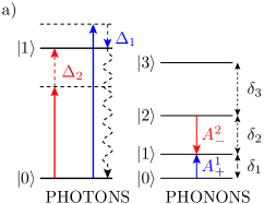
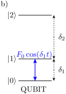
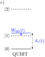
Figure 5: Different schemes for resonant interactions. a) Interaction between mechanical excitations and detuned photons entering the cavity. b) and c) interaction between a classical gradient field and mechanical excitations.

IX Measurement via output power spectrum

The steady state of a nanoresonator can be probed with an additional laser, weakly driving one cavity mode on resonance, i.e. with $\Delta=0$. Then, information about the state of the mechanical resonator can be extracted from the sideband structures in the power spectrum, which correspond to photons that have been up- or down converted during the interaction with the mechanical motion. The intensity of the sideband peaks depends on the population of the mechanical energy eigenstates. Thus, the power spectrum only provides information about the diagonal entries $P_{n}$ of the density matrix describing the mechanical resonator represented in the basis formed by eigenstates of the Hamiltonian $H_{\mathrm{m}}$, see Eq. (24). For a probe laser resonantly driving a cavity mode at frequency $\omega_{\mathrm{L}}$, the spectrum shows a sideband structure

$$S(\omega)=\sum\limits_{nm}\frac{\kappa_{\mathrm{ex}}|g_{\mathrm{m}}|^{2}}{4\delta_{nm}^{2}+\kappa^{2}}X_{nm}^{2}\text{L}_{nm}(\omega)P_{n}\,,$$ (73)

with Lorentzian sideband peaks determined by

$$\text{L}_{nm}(\omega)=\frac{1}{\pi}\frac{\gamma_{\mathrm{eff}}^{nm}/2}{\left[\omega-\omega_{\mathrm{L}}-\delta_{nm}\right]^{2}+(\gamma_{\mathrm{eff}}^{nm}/2)^{2}}\,,$$ (74)

with $\gamma_{\mathrm{eff}}$ as given in equation (B), see appendix B for details. Here, $g_{\mathrm{m}}$ is the optomechanical coupling strength associated with the probe laser and the $\delta_{nm}=(E_{n}-E_{m})/\hbar$ denote the mechanical transition frequencies. The peaks appear in groups with $n\!-\!m=1,3,...$; see figure 6. The occupation probabilities $P_{n}$ for the eigenstates $|n\rangle$ can be extracted from the peak intensities within the main sidebands with $n\!-\!m=1$ Rips2012 .

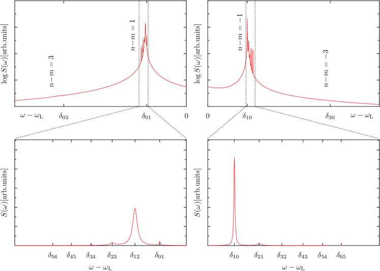
Figure 6: Output spectrum characterizing a motional state of a single nanoresonator where only the lowest few states are populated. Here, $P_{0}=0.0391$, $P_{1}=0.9137$, $P_{2}=0.0430$, $P_{3}=0.0024$, $P_{4}=0.0006$, $P_{5}=0.0003$ and $P_{j}<0.0003$ for $j>5$. Due to the parity of $\mathcal{X}$, there are only sideband groups at frequencies that correspond to processes where an odd number of phonons is scattered. The sidebands drop quickly in intensity with growing distance to the main line. The fine structure of the $n\!-\!m=\pm 1$ groups gives information about the level population of the resonator. The frequency axis is labeled in terms of the mechanical transition frequencies $\delta_{nm}$, and a peak at $\omega-\omega_{\mathrm{L}}=\delta_{mn}$ with $\delta_{mn}>0$ ($\delta_{mn}<0$) corresponds to anti-Stokes (Stokes) photon scattering events that occur at a rate proportional to the occupation of the respective initial mechanical level. In this example the level spacings correspond to a $1\text{\,}\mathrm{\SIUnitSymbolMicro m}$ length $(10,0)$ CNT that is softened so that $\omega_{\mathrm{m}}/2\pi=$5.23\text{\,}\mathrm{MHz}$$, which leads to $\delta_{10}\approx\lambda^{\prime}=$209\text{\,}\mathrm{kHz}$$. Three “active” state-preparation lasers with detunings $\Delta_{1}\approx\delta_{10}$, $\Delta_{2}\approx\delta_{12}$ and $\Delta_{3}\approx\delta_{23}$ induce optomechanical couplings $g_{\mathrm{m},1}=g_{\mathrm{m},2}=g_{\mathrm{m},3}=$20.9\text{\,}\mathrm{kHz}$$ —for the parameters considered (cf. Section V) this value can be achieved keeping the intracavity absorption in the microwatt range Rips2012 . The resulting optomechanical interactions with the nanobeam dominate over the intrinsic mechanical decoherence rates and determine the broadening of the levels involved, see section B —the remaining relevant parameters are: $\kappa_{\mathrm{ex}}/\kappa=0.1$, $\kappa_{1}/2\pi=\kappa_{2}/2\pi=\kappa_{3}/2\pi=52.3\,$kHz, $\omega_{\mathrm{m}}/\gamma=5\times 10^{6}$ and $T=20\,$mK.

For the readout of mechanical qubits as discussed in Rips2013 , a shelving technique can be used to determine whether a qubit is in state $|0\rangle$ or in state $|1\rangle$. Here, a balanced cycling transition between $|1\rangle\leftrightarrow|2\rangle$ using a cooling laser on $|2\rangle\rightarrow|1\rangle$ and a coherent rf-drive with local gradient fields on those two levels causes a continuous stream of up converted photons only if the resonator is found in the state $|1\rangle$. This can be detected by measuring the corresponding sideband spectrum. Here, a large enough number of photons has to be collected before external damping destroys the intermediate state, which requires $\kappa_{\mathrm{ex}}|g_{\mathrm{m}}|^{2}/\kappa^{2}\gg\gamma\overline{n}$.

X Conclusions and Outlook

We have introduced a scheme to access a novel regime of optomechanics where the motion of the nanomechanical resonator becomes anharmonic and thus allows to explore genuine quantum dynamics. In our approach inhomogeneous electrostatic fields are applied to the nanomechanical resonator to enhance its anharmonicity per phonon until it becomes comparable to the linewidth of a high finesse optical cavity. For realistic experimental conditions, sufficiently large optomechanical couplings can be realized and losses induced by the tip electrodes can be suppressed to a negligible level. Furthermore populations of the energy eigenstates of such nonlinear mechanical oscillators can be extracted from the output spectrum of a probe laser. The approach thus paves the way towards exploring nonclassical dynamics of nanomechanical oscillators at the single-phonon level.

XI Acknowledgements

This work is part of the Emmy Noether project HA 5593/1-1 and was supported the CRC 631, both funded by the German Science Foundation (DFG). IWR acknowledges support by the German Science Foundation (DFG) via the grant WI 3859/1-1 and Nanosystems Initiative Munich (NIM). The authors thank J. Kotthaus, T.J. Kippenberg, and A. Schliesser for enlightening discussions.

Appendix A Corrections due to nonlinear mode coupling

In order to estimate the strength of the mode coupling, we rewrite the nonlinearity (11) as

$$\lambda_{ijkl}^{0}=\frac{\hbar}{32\tilde{\kappa}^{2}m}\left[\frac{\mu^{2}L^{2}\tilde{M}_{ij}\tilde{M}_{lk}}{\sqrt{m^{*}_{i}m^{*}_{j}m^{*}_{k}m^{*}_{l}}\nu_{i}\nu_{j}\nu_{k}\nu_{l}}\right]\,,$$ (75)

where $m=\mu L$ is the physical mass of the rod. The term in brackets solely depends on the mode shape for the doubly clamped boundary conditions and is independent of the parameters $\tilde{\kappa}$, $\mu$, $L$, of the oscillator. This can be seen from substituting $\tilde{\phi}_{n}(\tilde{x})\equiv\phi_{n}(L\tilde{x})$, which yields

$$\tilde{M}_{ij} =LM_{ij}=\int_{0}^{1}\tilde{\phi}_{i}^{\prime}\tilde{\phi}_{j}^{\prime}{\rm d}\tilde{x}\,,$$ (76)

$$m^{*}_{n} =\mu L\int_{0}^{1}\tilde{\phi}_{n}^{2}{\rm d}\tilde{x}\,.$$ (77)

Table 1 shows some numerically obtained values for the bracket in equation (75) that are relevant for the fundamental mode. In the case of an electrostatically tuned resonator, the modified nonlinear couplings read

$$\lambda_{ijkl}=\lambda^{0}_{ijkl}\sqrt{\zeta_{i}\zeta_{j}\zeta_{k}\zeta_{l}}\,,$$ (78)

where $\zeta_{i}=\omega_{i,0}/\omega_{i}$ is the factor by which the frequency of mode $i$ is reduced due to the presence of the gradient fields. While this factor is usually intended to be larger than unity for the fundamental mode $\zeta_{1}\sim 10$, it remains close to unity for the higher modes.

Phonon transfer between modes is strongly suppressed because of resonance mismatches, as $\lambda_{ijkl}\ll\sum_{n=ijkl}(\pm\omega_{n})$ for processes where the phonon number in each mode is not preserved. One should note that the relevant frequency ratios scale as $\lambda_{0}/\omega_{\mathrm{m},0}\ll 1$ and the dominant processes of this type affecting the fundamental mode involve its coupling to the next higher mode with the same symmetry, which is the third mode. In addition, the fundamental mode experiences a modification of its rigidity due to the thermal and quantum fluctuations of higher order modes with $\omega_{n}<\omega_{N}\sim c_{\mathrm{s}}\pi/L$. This effect however can be taken into account by a proper redefinition of the fundamental mode’s rigidity.

$j\diagdown i$	$1$	$2$	$3$	$4$	$5$
$1$	0.3024	—	0.1029	—	-0.0512
$2$	—	0.4106	—	-0.0848	—
$3$	0.1029	—	0.4498	—	0.0705
$4$	—	-0.0848	—	0.4721	—
$5$	-0.0512	—	0.0705	—	0.486232

Table 1: $32\tilde{\kappa}^{2}m\lambda_{11ij}^{0}/\hbar$. Only pairs of modes $i,j$ with the same parity yield a finite coupling of this type.

Appendix B Output power spectrum

A steady state of the mechanical resonator can be probed via a resonant laser drive on an additional cavity mode. The quantum motion of the nanoresonator is described by the reduced master equation Rips2012 ,

$$\dot{\mu}\approx-\mathrm{i}\left[\sum\limits_{n}E_{n}|n\rangle\langle n|,\mu\right]+\frac{1}{2}\sum\limits_{nm,j}A^{nm}_{j}\mathcal{D}(|n\rangle\langle m|)\mu+\mathcal{D}_{\gamma}\mu\,.$$ (79)

Here, $\mathcal{D}_{\gamma}\mu$ includes the external mechanical damping via standard Lindblad terms and the influence of the lasers is given by the rates

$$A^{nm}_{j}=|g_{\mathrm{m},j}|^{2}\frac{X_{nm}^{2}\kappa_{j}}{4\left(\Delta_{j}-\delta_{nm}\right)^{2}+\kappa_{j}^{2}}\,.$$ (80)

Here, for example, $j=0$ labels the probe laser with $\Delta_{0}=0$ and the other lasers with $j=1,2,...$ are used for the steady state preparation, see Section VIII. The rates $A^{nm}_{0}$ have to be small, i.e. $A^{nm}_{0}\lesssim\gamma\overline{n}$, to assure a weak measurement. The output power spectrum is given by

$$S(\omega)\!=\!\sum\limits_{j}\!\frac{1}{2\pi}\!\!\int\limits_{-\infty}^{\infty}\!\!\mathrm{d}\tau\mathrm{e}^{-\mathrm{i}(\omega-\omega_{\mathrm{L},j})\tau}\!\left.\left\langle a_{\mathrm{out},j}^{{\dagger}}(t+\tau)a_{\mathrm{out},j}(t)\right\rangle\right|_{\mathrm{SS}}$$ (81)

where the output fields $a_{\mathrm{out},j}(t)$ are related to the intracavity fields $a_{j}(t)$ via the standard input-output relation PhysRevA.31.3761 ,

$$a_{\mathrm{out},j}=\sqrt{\kappa_{\mathrm{ex}}}a_{j}+a_{\mathrm{in},j}\,.$$ (82)

Here, we only focus on the output for the probe field and thus drop the index $j$. The dynamics of the intra cavity field can be described by a quantum Langevin equation

$$\dot{a}= -\frac{\kappa}{2}a-\mathrm{i}G_{0}x_{\mathrm{ZPM}}\left(b^{{\dagger}}+b\right)\left(a+\alpha\right)$$

$$+\sqrt{\kappa_{\mathrm{ex}}}\delta a_{\mathrm{in}}(t)+\sqrt{\kappa-\kappa_{\mathrm{ex}}}\delta c_{\mathrm{in}}(t)\,,$$ (83)

where $\delta a_{\mathrm{in}}$ and $\delta c_{\mathrm{in}}$ are the fluctuations of the input field in the laser mode and the other bath modes. Defining $a^{(0)}$ to be a solution for $G_{0}=0$, we can integrate (83) formally and apply a Dyson series type expansion to first order in the optomechanical coupling strength $g_{\mathrm{m}}$, to find for the motion of the cavity modes, cf. 1367-2630-10-9-095007 ,

$$a(t) \approx a^{(0)}(t)-\mathrm{i}\frac{g_{\mathrm{m}}}{2}\int\limits_{0}^{t}\mathrm{d}\tau\mathrm{e}^{-\frac{\kappa}{2}(t-\tau)}\left[b^{{\dagger}}(\tau)+b(\tau)\right]$$

$$\approx a^{(0)}(t)-\mathrm{i}\frac{g_{\mathrm{m}}}{2}\sum\limits_{n<m}X_{nm}\left[\frac{|n\rangle\langle m|(t)}{\mathrm{i}\delta_{nm}-\kappa/2}+\text{H.c.}\right]\,.$$ (84)

The contribution of the fluctuations is included in the free field solution $a^{(0)}(t)$ and the input field operators have already been written in a shifted representation $a_{\mathrm{in}}(t)\rightarrow\delta a_{\mathrm{in}}(t)+\left\langle a_{\mathrm{in}}\right\rangle$, which splits off the coherent part of the input. We substitute (82) and (84) into (81) and concentrate on the contributions to the sidebands, which to lowest order in $g_{\mathrm{m}}/\omega_{\mathrm{m}}$ are given by the first order two-time correlations of the mechanical motion. The latter can be calculated from the reduced master equation (79) using the quantum regression theorem. We find that

$$\big{\langle}|n\rangle\langle m|(t+\tau)|m\rangle\langle n|(t)\big{\rangle}=\mathrm{e}^{\left(\mathrm{i}\delta_{nm}-\gamma_{\mathrm{eff}}^{nm}/2\right)\tau}P_{n}\,,$$ (85)

where $P_{n}=\langle n|\mu|_{\mathrm{SS}}|n\rangle$ are the probabilities to find the resonator in the eigenstate $|n\rangle$, are the only nonvanishing contributions. Thus the sideband spectrum around the probe laser frequency reads

$$S(\omega)=\frac{\kappa_{\mathrm{ex}}}{2\pi\kappa}\sum_{nm}\frac{A^{nm}_{0}\gamma_{\mathrm{eff}}^{nm}}{\left(\omega-\omega_{\mathrm{L}}-\delta_{nm}\right)^{2}+\left(\gamma_{\mathrm{eff}}^{nm}\right)^{2}/4}P_{n}\,.$$ (86)

The resulting peak linewidths

$$\gamma_{\mathrm{eff}}^{nm}= \sum\limits_{l,j}\left(A^{lm}_{j}+A^{ln}_{j}\right)+\gamma\overline{n}\left(\sum\limits_{k>m}X_{km}^{2}+\sum\limits_{k>n}X_{kn}^{2}\right)$$

$$+\gamma(\overline{n}+1)\left(\sum\limits_{l<m}X_{lm}^{2}+\sum\limits_{l<n}X_{ln}^{2}\right)$$ (87)

satisfy $\gamma_{\mathrm{eff}}^{nm}\ll\lambda$, where the nonlinearity $\lambda$ is the typical peak distance within the fine structure of one sideband, see figure 6.

References

- (1) S. Rips, M. Kiffner, I. Wilson-Rae and M. J. Hartmann, New J. Phys. 14, 023042 (2012).
- (2) S. Rips and M. J. Hartmann, Phys. Rev. Lett. 110, 120503 (2013).
- (3) T. Rocheleau, T. Ndukum, C. Macklin, J.B. Hertzberg, A.A. Clerk, and K.C. Schwab, Nature 463, 72 (2010).
- (4) A.D. O’Connell, M. Hofheinz, M. Ansmann, R.C. Bialczak, M. Lenander, E. Lucero, M. Neeley, D. Sank, H. Wang, M. Weides, J. Wenner, J.M. Martinis and A.N. Cleland, Nature 464, 697 (2010).
- (5) J.D. Teufel, T. Donner, Dale Li, J.H. Harlow, M.S. Allman, K. Cicak, A.J. Sirois, J.D. Whittaker, K.W. Lehnert, and R.W. Simmonds, Nature 475, 359 (2011).
- (6) J. Chan, T.P. Mayer Alegre, A.H. Safavi-Naeini, J.T. Hill, A. Krause, S. Gröblacher, M. Aspelmeyer, and O. Painter, Nature 478, 89 (2011).
- (7) E. Verhagen, S. Deleglise, S. Weis, A. Schliesser, and T. J. Kippenberg, Nature 482, 63 (2012).
- (8) T. J. Kippenberg and K. J. Vahala, Science 321, 1172 (2008)
- (9) A.D. Armour, M.P. Blencowe, and K.C. Schwab, Phys. Rev. Lett. 88, 148301 (2002).
- (10) F. Marquardt and S.M. Girvin, Physics 2, 40 (2009).
- (11) J.D. Teufel, T. Donner, M.A. Castellanos-Beltran, J.W. Harlow, and K.W. Lehnert, Nature Nanotech. 4, 820 (2009).
- (12) A. Schliesser, R. Riviére, G. Anetsberger, O. Arcizet, T.J. Kippenberg, Nat. Phys. 5, 509 (2009).
- (13) G. Anetsberger, E. Gavartin, O. Arcizet, Q.P. Unterreithmeier, E.M. Weig, M.L. Gorodetsky, J.P. Kotthaus, T.J. Kippenberg, Phys. Rev. A 82, 061804 (2010).
- (14) S.L. Adler and A. Bassi, Science 325, 275 (2009).
- (15) M. Aspelmeyer, T. J. Kippenberg, F. Marquardt, arXiv:1303.0733 (2013).
- (16) P. Ehrenfest, Z. Phys. A 45, 455 (1927).
- (17) P. Rabl, Phys. Rev. Lett. 107, 063601 (2011).
- (18) A. Nunnenkamp, K. Borkje, and S. M. Girvin, Phys. Rev. Lett. 107, 063602 (2011).
- (19) J. C. Sankey, C. Yang, B. M. Zwickl, A. M. Jayich and J. G. E. Harris, Nat. Phys. 6 707 (2010)
- (20) K. Jacobs, Phys. Rev. Lett. 99, 117203 (2007).
- (21) S.M. Carr, W.E. Lawrence, and M.N. Wybourne, Phys. Rev. B 64, 220101 (2001).
- (22) V. Peano and M. Thorwart, New J. Phys. 8, 21 (2006).
- (23) E. Babourina-Brooks, A. Doherty and G.J. Milburn, New J. Phys. 10, 105020 (2008).
- (24) I. Katz, A. Retzker, R. Straub, and R. Lifshitz, Phys. Rev. Lett. 99, 040404 (2007).
- (25) M.J. Hartmann and M.B. Plenio, Phys. Rev. Lett. 101, 200503 (2008).
- (26) M.I. Dykman, M. Marthaler, and V. Peano, Phys. Rev. A 83, 052115 (2011).
- (27) Q.P. Unterreithmeier, E.M. Weig, and J.P. Kotthaus, Nature 458, 1001 (2009).
- (28) L.D. Landau and E.M. Lifshitz, Theory of elasticity, Pergamon, Oxford (1986).
- (29) P. Werner and W. Zwerger, Europhys. Lett.65 (2004).
- (30) G. Anetsberger, O. Arcizet, Q.P. Unterreithmeier, R. Riviére, A. Schliesser, E.M. Weig, J.P. Kotthaus, and T.J. Kippenberg, Nat. Phys. 5, 909 (2009).
- (31) M. Pöllinger, D. O’Shea, F. Warken and A. Rauschenbeutel, Phys. Rev. Lett. 103, 053901 (2009).
- (32) K. H. Lee, T. G. McRae, G.I. Harris, J. Knittel, and W. P. Bowen, Phys. Rev. Lett. 104, 123604 (2010).
- (33) G.A. Steele, A.K. Hüttel, B. Witkamp, M. Poot, H.B. Meerwaldt, L.P. Kouwenhoven, and H.S.J. van der Zant, Science 325, 1103 (2009).
- (34) B. Lassagne, Y. Tarakanov, J. Kinaret, D. Garcia-Sanchez, and A. Bachtold, Science 325, 1107 (2009).
- (35) M. S. Hofmann, J. T. Glückert, J. Noe, C. Bourjau, R. Dehmel, and A. Hogele, Nature Nanotech. 8, 502 (2013).
- (36) J. Waissman, M. Honig, S. Pecker, A. Benyamini, A. Hamo, and S. Ilani, Nature Nanotech. 8, 569 (2013).
- (37) S. Stapfner, L. Ost, D. Hunger, J. Reichel, I. Favero, and E. M. Weig, Appl. Phys. Lett. 102, 151910 (2013).
- (38) A.K. Hüttel, G.A. Steele, B. Witkamp, M. Poot, L.P. Kouwenhoven and H.S.J. van der Zant, Nano Lett. 9, 2547 (2009).
- (39) A. Eichler, J. Moser, J. Chaste, M. Zdrojek, I. Wilson-Rae, and A. Bachtold, Nature Nanotech. 6, 339 (2011).
- (40) B. Kozinsky and N. Marzari, Phys. Rev. Lett. 96, 166801 (2006).
- (41) T. J. Kippenberg, S. M. Spillane, and K. J. Vahala, App. Phys. Lett. 85, 6113 (2004)
- (42) J. D. Jackson, Classical Electrodynamics, Wiley, New York (1998)
- (43) I. Wilson-Rae, Phys. Rev. B 77, 245418 (2008).
- (44) L. G. Remus, M. P. Blencowe, and Y. Tanaka, Phys. Rev. B 80, 174103 (2009).
- (45) D.Y. Joh, J. Kinder, L.H. Herman, S.-Y. Ju, M.A. Segal, J.N. Johnson, G.K.-L. Chan and J. Park, Nature Nanotech. 6, 51 (2011).
- (46) H. Nyquist, Phys. Rev. Lett. 32, 110 (1928)
- (47) B. C. Stipe, H. J. Mamin, T. D. Stowe, T. W. Kenny, and D. Rugar, Phys. Rev. Lett. 87, 096801 (2001).
- (48) P. Rabl, S. J. Kolkowitz, F. H. L. Koppens, J. G. E. Harris, P. Zoller, and M. D. Lukin, Nat. Phys. 6, 602 (2010).
- (49) I. Wilson-Rae, C. Galland, W. Zwerger, and A. Imamoğlu, New J. Phys. 14, 115003 (2012)
- (50) I. Wilson-Rae, N. Nooshi, W. Zwerger, and T.J. Kippenberg, Phys. Rev. Lett. 99, 093901 (2007).
- (51) F. Marquardt, J.P. Chen, A.A. Clerk, and S.M. Girvin, Phys. Rev. Lett. 99, 093902 (2007).
- (52) C. W. Gardiner and M. J. Collett, Phys. Rev. A 31, 3761 (1985)
- (53) I. Wilson-Rae, N. Nooshi, J. Dobrindt, T.J. Kippenberg, and W. Zwerger, New J. Phys. 10, 095007 (2008).